Validation Metrics for Continuous Variables: A 2025 Guide for Robust Biomedical Research and Drug Development

Abstract

This article provides a comprehensive framework for selecting, applying, and interpreting validation metrics for continuous variables in biomedical and clinical research. Tailored for scientists and drug development professionals, it bridges foundational statistical theory with practical application, covering essential parametric tests, advanced measurement systems like Gage R&R, data quality best practices, and modern digital validation trends. Readers will gain the knowledge to ensure data integrity, optimize analytical processes, and make statistically sound decisions in regulated environments.

Laying the Groundwork: Core Principles of Continuous Data and Validation

In the context of validation metrics for continuous variables research, understanding the fundamental nature of continuous data is paramount. Continuous data represent measurements that can take on any value within a given range, providing an infinite number of possible values and allowing for meaningful division into smaller increments, including fractional and decimal values [1]. This contrasts with discrete data, which consists of distinct, separate values that are counted. In scientific and drug development research, common examples of continuous data include blood pressure measurements, ejection fraction, laboratory values (e.g., cholesterol), angiographic variables, weight, temperature, and time [2] [3].

The power of continuous data lies in the depth of insight it provides. Researchers can draw conclusions with smaller sample sizes compared to discrete data and employ a wider variety of analytical techniques [3]. This rich information allows for more accurate predictions and deeper insights, which is particularly valuable in fields like drug development where precise measurements can determine treatment efficacy and safety. The fluid nature of continuous data captures the subtle nuances of biological systems in a way that discrete data points cannot, making it indispensable for robust validation metrics.

Measures of Central Tendency: Mean, Median, and Mode

Measures of central tendency are summary statistics that represent the center point or typical value of a dataset. The three most common measures are the mean, median, and mode, each with a distinct method of calculation and appropriate use cases within research on continuous variables [4] [5].

Definitions and Calculations

• Mean (μ or x̄): The arithmetic average, calculated as the sum of all values divided by the number of values in the dataset (Σx/n) [4] [5]. The mean includes every value in your data set as part of the calculation and is the value that produces the lowest amount of error from all other values in the data set [4].
• Median: The middle value that separates the greater and lesser halves of a dataset. To find it, data is ordered from smallest to largest. For an odd number of observations, it is the middle value; for an even number, it is the average of the two middle values [4] [5].
• Mode: The value that appears most frequently in a dataset [6]. For continuous data in its raw form, the mode is often unusable as no two values may be exactly the same. A common practice is to discretize the data into intervals, as in a histogram, and define the mode as the midpoint of the interval with the highest frequency [6].

Comparative Analysis: Mean vs. Median

The choice between mean and median is critical and depends heavily on the distribution of the data, a key consideration when establishing validation metrics.

Table 1: Comparison of Mean and Median as Measures of Central Tendency

Characteristic	Mean	Median
Definition	Arithmetic average	Middle value in an ordered dataset
Effect of Outliers	Highly sensitive; pulled strongly in the direction of the tail [5]	Robust; resistant to the influence of outliers and skewed data [4] [5]
Data Utilization	Incorporates every value in the dataset [4]	Depends only on the middle value(s) [5]
Best Used For	Symmetric distributions (e.g., normal distribution) [4] [5]	Skewed distributions [4] [5]
Typical Data Reported	Mean and Standard Deviation (SD) [2]	Median and percentiles (e.g., 25th, 75th) or range [2]

In a perfectly symmetrical, unimodal distribution (like the normal distribution), the mean, median, and mode are all identical [4] [6]. However, in skewed distributions, these measures diverge. The mean is dragged in the direction of the skew by the long tail of outliers, while the median remains closer to the majority of the data [4] [5]. A classic example is household income, which is typically right-skewed (a few very high incomes); in such cases, the median provides a better representation of the "typical" income than the mean [5].

Assessing Data Distribution and Its Implications

The distribution of data is a foundational concept that directly influences the choice of descriptive statistics and inferential tests. For continuous data, the most frequently assessed distribution is the normal distribution (bell curve), which is symmetric and unimodal [2].

Normality Assessment Workflow

Determining whether a continuous variable is normally distributed is a crucial step in selecting the correct analytical pathway. The following diagram outlines the key steps and considerations in this process.

Methodologies for Normality Testing

As shown in the workflow, assessing normality involves both graphical and formal statistical methods, which are integral to robust experimental protocols:

• Graphical Methods: Visual examination of data is a primary step. Researchers can use histograms to see if the data resembles a bell-shaped curve, box plots to assess symmetry and identify outliers, and Q-Q plots (Quantile-Quantile plots) where data points aligning closely with the diagonal line suggest normality [2].
• Statistical Tests: Formal hypothesis tests provide an objective measure. Commonly used tests include the Kolmogorov-Smirnov test and the Shapiro-Wilk test [2]. A p-value greater than the significance level (e.g., > 0.05) in these tests suggests that the data does not significantly deviate from a normal distribution.

Statistical Significance Testing for Continuous Data

Once the distribution is understood, researchers can select appropriate tests to determine statistical significance—the probability that an observed effect is not due to random chance alone.

Hypothesis Testing Framework

The foundation of these tests is the null hypothesis (H₀), which typically states "there is no difference" between groups or "no effect" of a treatment. The alternative hypothesis (H₁) states that a difference or effect exists. The p-value quantifies the probability of obtaining the observed results if the null hypothesis were true. A p-value less than a pre-defined significance level (alpha, commonly 0.05) provides evidence to reject the null hypothesis [2].

Guide to Selecting Statistical Tests

The choice of statistical test is dictated by the number of groups being compared and the distribution of the continuous outcome variable.

Table 2: Statistical Tests for Comparing Continuous Variables

Number of Groups	Group Relationship	Parametric Test (Data ~Normal)	Non-Parametric Test (Data ~Non-Normal)
One Sample	-	One-sample t-test [7]	One-sample sign test or median test [7]
Two Samples	Independent (Unpaired)	Independent (unpaired) two-sample t-test [2] [7]	Mann-Whitney U test [7]
Two Samples	Dependent (Paired)	Paired t-test [2] [7]	Wilcoxon signed-rank test [7]
Three or More Samples	Independent (Unpaired)	One-way ANOVA [2] [7]	Kruskal-Wallis test [7]
Three or More Samples	Dependent (Paired)	Repeated measures ANOVA [7]	Friedman test [7]

Key Assumptions and Applications

• T-test: A commonly used parametric test to compare means. Its assumptions include: data derived from a normally distributed population, for two-sample tests the populations must have equal variances, and all measurements must be independent [2]. It is used to compare a sample mean to a theoretical value (one-sample), compare means from two related groups (paired), or compare means from two independent groups (independent) [2].
• ANOVA (Analysis of Variance): Used to test for differences among three or more group means, extending the capability of the t-test. Using multiple t-tests for more than two groups increases the probability of a Type I error (falsely rejecting the null hypothesis), which ANOVA controls [2]. A significant ANOVA result (p < 0.05) indicates that not all group means are equal, but it does not specify which pairs differ, necessitating a post-hoc test (e.g., Tukey's test) for further investigation [7].
• Non-Parametric Tests: These are used when data violates the normality assumption, particularly with small sample sizes or ordinal data. They are typically based on ranks of the data rather than the actual values and are thus less powerful than their parametric counterparts but more robust to outliers and non-normality [2] [7].

The Researcher's Toolkit for Continuous Data Analysis

Successfully analyzing continuous data in validation studies requires more than just statistical knowledge; it involves a suite of conceptual and practical tools.

Table 3: Essential Toolkit for Analyzing Continuous Variables

Tool or Concept	Function & Purpose
Measures of Central Tendency	To summarize the typical or central value in a dataset (Mean, Median, Mode) [4] [5].
Measures of Variability	To quantify the spread or dispersion of data points (e.g., Standard Deviation, Range, Interquartile Range) [2].
Normality Tests	To objectively assess if data follows a normal distribution, guiding test selection (e.g., Shapiro-Wilk test) [2].
Data Visualization Software	To create histograms, box plots, and Q-Q plots for visual assessment of distribution and outliers [8].
Statistical Software	To perform complex calculations for hypothesis tests (e.g., R, SPSS, Python with SciPy/Statsmodels) [7].
Tolerance Intervals / Capability Analysis	To understand the range where a specific proportion of the population falls and to assess process performance against specification limits, respectively [3].

The rigorous analysis of continuous data forms the bedrock of validation metrics in scientific and drug development research. A meticulous approach that begins with visualizing and understanding the data distribution, followed by the informed selection of descriptive statistics (mean vs. median) and inferential tests (parametric vs. non-parametric), is critical for drawing valid and reliable conclusions. By adhering to this structured methodology—assessing normality, choosing robust measures of central tendency, and applying the correct significance tests—researchers can ensure their findings accurately reflect underlying biological phenomena and support the development of safe and effective therapeutics.

The Critical Role of Validation in Research and Regulated Environments

Validation provides the critical foundation for trust and reliability in both research and regulated industries. It encompasses the processes, tools, and metrics used to ensure that systems, methods, and data consistently produce results that are fit for their intended purpose. In 2025, validation has become more business-critical than ever, with teams facing increasing scrutiny from regulators and growing complexity in global regulatory requirements [9]. The validation landscape is undergoing a significant transformation, driven by the adoption of digital tools, evolving regulatory priorities, and the need to manage more complex workloads with limited resources.

This transformation is particularly evident in life sciences and clinical research, where proper validation is essential for ensuring data integrity, patient safety, and compliance with Good Clinical Practices (GCP) and FDA 21 CFR Part 11 [10]. Without rigorous validation, clinical data may be compromised, resulting in delays, increased costs, and potentially jeopardizing patient safety. The expanding scale of regulatory change presents a formidable challenge, with over 40,000 individual regulatory items issued at federal and state levels annually, requiring organizations to identify, analyze, and determine applicability to their business operations [11].

Current Challenges in Validation

Validation teams in 2025 face a complex set of challenges that reflect the increasing demands of regulatory environments and resource constraints.

Primary Validation Team Challenges

A comprehensive analysis of the validation landscape reveals three dominant challenges that teams currently face [9] [12]:

• Audit Readiness: For the first time in four years, audit readiness has emerged as the top challenge for validation teams, surpassing compliance burden and data integrity. Organizations are now expected to demonstrate a constant state of preparedness as global regulatory requirements grow more complex [9] [12].

• Compliance Burden: The expanding regulatory landscape creates significant compliance obligations, with firms across insurance, securities, and investment sectors facing a steady stream of new requirements fueled by shifting federal priorities, proactive state legislatures, and emerging risks tied to climate, technology, and cybersecurity [11].

• Data Integrity: Ensuring the accuracy and consistency of data throughout its lifecycle remains a fundamental challenge, particularly as organizations adopt more complex digital systems and face increased scrutiny from regulatory bodies [9].

Resource Constraints and Workload Pressures

Compounding these challenges, validation teams operate with limited resources while managing increasing workloads [12]:

• Lean Team Structures: 39% of companies report having fewer than three dedicated validation staff, despite increasingly complex regulatory workloads [9] [12].

• Growing Workloads: 66% of organizations report that their validation workload has increased over the past 12 months, creating significant pressure on already constrained resources [9] [12].

• Strategic Outsourcing: 70% of companies now rely on external partners for at least some portion of their validation work, with 25% of organizations outsourcing more than a quarter of their validation activities [12].

Table 1: Primary Challenges Facing Validation Teams in 2025

Rank	Challenge	Description
1	Audit Readiness	Maintaining constant state of preparedness for regulatory inspections
2	Compliance Burden	Managing complex and evolving regulatory requirements
3	Data Integrity	Ensuring accuracy and consistency of data throughout its lifecycle

Table 2: Validation Team Resource Constraints

Constraint Type	Statistic	Impact
Small Team Size	39% of companies have <3 dedicated validation staff	Limited capacity for complex workloads
Increased Workload	66% report year-over-year workload increase	Resource strain and potential burnout
Outsourcing Dependence	70% use external partners for some validation work	Need for specialized expertise access

Digital Transformation in Validation

The adoption of Digital Validation Tools (DVTs) represents a fundamental shift in how organizations approach validation, with 2025 marking a tipping point for the industry.

Adoption Trends and Benefits

Digital validation systems have seen remarkable adoption rates, with the number of organizations using these tools jumping from 30% to 58% in just one year [9]. Another 35% of organizations are planning to adopt DVTs in the next two years, meaning nearly every organization (93%) is either using or actively planning to use digital validation tools [9]. This massive shift is driven by the substantial advantages these systems offer, including centralized data access, streamlined document workflows, support for continuous inspection readiness, and enhanced efficiency, consistency, and compliance across validation programs [9].

Survey respondents specifically cited data integrity and audit readiness as the two most valuable benefits of digitalizing validation, directly addressing the top challenges facing validation teams [9]. The move toward digital validation is part of a broader industry transformation that includes the adoption of advanced strategies such as automated testing, continuous validation, risk-based validation, and AI-driven analytics [10].

Advanced Validation Strategies for 2025

Several advanced approaches are enhancing validation processes in 2025 and beyond [10]:

• Automated Testing and Validation Tools: Automation streamlines repetitive tasks, improves accuracy, and ensures consistency while accelerating validation cycles. Automated validation frameworks can generate test cases based on User Requirements Specification documents, execute tests across different environments, and produce detailed reports [10].

• Continuous Validation (CV) Approach: This strategy integrates validation into the software development lifecycle (SDLC), ensuring that each new feature or update undergoes validation in real-time. This proactive approach minimizes the risk of errors and reduces the need for large-scale re-validation efforts [10].

• Risk-Based Validation (RBV): This methodology focuses resources on high-risk areas, allowing organizations to allocate their efforts strategically. In electronic systems, modules dealing with patient randomization, adverse event reporting, and electronic signatures typically warrant extensive validation, while lower-risk elements may undergo lighter validation [10].

• AI and Machine Learning Integration: Artificial intelligence tools can analyze large datasets for anomalies, identify discrepancies, and predict potential errors. AI-driven analytics enhance data integrity by flagging irregularities that may escape manual review and can automate audit trail reviews and compliance reporting [10].

Table 3: Digital Validation Tool Adoption Trends

Adoption Stage	Percentage of Organizations	Key Driver
Currently Using DVTs	58%	Audit readiness and data integrity
Planning to Adopt (Next 2 Years)	35%	Efficiency and compliance needs
Total Engaged with DVTs	93%	Industry tipping point reached

Validation Metrics and Methodologies

Robust validation requires appropriate metrics and methodologies to ensure systems perform as intended across various applications and use cases.

Validation Metrics for Clinical Research Hypotheses

In clinical research, validated metrics provide standardized, consistent, and systematic measurements for evaluating scientific hypotheses. Recent research has developed both brief and comprehensive versions of evaluation instruments [13]:

The brief version of the instrument contains three core dimensions:

• Validity: Assesses clinical validity and scientific validity
• Significance: Evaluates established medical needs, impact on future direction of the field, effect on target population, and cost-benefit considerations
• Feasibility: Examines required costs, needed time, and scope of work

The comprehensive version includes these three dimensions plus additional criteria:

• Novelty: Leads to innovation in medical practice, new methodologies for clinical research, alteration of previous findings, novel medical knowledge, or incremental new findings
• Clinical Relevance: Impact on current clinical practice, medical knowledge, and health policy
• Potential Benefits and Risks: Significant benefits, tolerable risks, and overall risk-benefit balance
• Ethicality: Absence of ethical concerns, willingness to participate if eligible, and overall ethical study design
• Testability: Ability to be tested in ideal settings with adequate patient population
• Interestingness: Personal interest and potential for collaboration
• Clarity: Clear purposes, focused groups, specified variables, and defined relationships among variables

Each evaluation dimension includes 2 to 5 subitems that assess specific aspects, with the brief and comprehensive versions containing 12 and 39 subitems respectively. Each subitem uses a 5-point Likert scale for consistent assessment [13].

Machine Learning Validation Metrics

For machine learning applications, different evaluation metrics are used depending on the specific task [14]:

• Binary Classification: Common metrics include accuracy, sensitivity (recall), specificity, precision, F1-score, Cohen's kappa, and Matthews' correlation coefficient (MCC). The receiver operating characteristic (ROC) curve and area under the curve (AUC) provide threshold-independent evaluation [14].

• Multi-class Classification: Approaches include macro-averaging (calculating metrics separately for each class then averaging) and micro-averaging (computing metrics from aggregate sums across all classes) [14].

• Regression: Continuous variables are analyzed using methods like linear regression and artificial neural networks, with cross-validation being essential for ensuring robustness of discovered patterns [15].

Statistical Considerations for Continuous Variables

The analysis of continuous variables requires particular methodological care. Categorizing continuous variables by grouping values into two or more categories creates significant problems, including considerable loss of statistical power and incomplete correction for confounding factors [16]. The use of data-derived "optimal" cut-points can lead to serious bias and should be tested on independent observations to assess validity [16].

Research demonstrates that 100 continuous observations are statistically equivalent to at least 157 dichotomized observations, highlighting the efficiency loss caused by categorization [16]. Furthermore, statistical models with a categorized exposure variable remove only 67% of the confounding controlled when the continuous version of the variable is used [16].

Digital vs Traditional Validation Workflow

Validation in Practice: Applications and Protocols

REDCap Validation in Clinical Research

REDCap (Research Electronic Data Capture) is widely adopted for its flexibility and capacity to manage complex clinical trial data, but requires thorough validation to ensure consistent and reliable performance [10]. The validation process involves several key components:

• User Requirements Specification (URS): Details all functional and non-functional requirements, including data entry forms, workflows, and reporting capabilities
• Risk Assessment: Identifies potential threats to data integrity, patient safety, and regulatory compliance
• Functional Testing: Rigorous examination of each module to ensure specified requirements are met
• Performance Testing: Simulates high-load conditions to verify system can handle large datasets and concurrent users
• Security Validation: Verifies role-based access controls, encryption mechanisms, and audit trails
• Data Migration Testing: Validates integrity of transferred data when migrating from legacy systems
• Audit Trail Review: Confirms all data modifications are logged accurately
• Change Control: Ensures system updates do not compromise validation status [10]

Shiny App Validation in Regulated Environments

Shiny applications present unique validation challenges due to their stateful, interactive, and user-driven nature [17]. Practical validation strategies include:

• Modular Code: Keeping UI and logic separate to enhance maintainability and testability
• Version Control: Using tools like Git to maintain environmental snapshots and track changes
• Comprehensive Testing: Implementing unit tests with testthat and end-to-end tests with shinytest2
• Environment Management: Using renv or Docker to freeze environments and ensure consistency
• Input Validation: Restricting and validating user inputs to prevent errors
• Comprehensive Logging: Implementing audit trails to track user actions and input history [17]

New Approach Methodologies (NAMs) Validation

The validation of New Approach Methodologies represents an emerging frontier, with initiatives like the Complement-ARIE public-private partnership aiming to accelerate the development and evaluation of NAMs for chemical safety assessments [18]. This collaboration focuses on:

• Establishing criteria for selecting specific NAMs for validation
• Obtaining community input on NAMs that meet readiness criteria
• Developing comprehensive procedures and protocols to transparently evaluate and document the robustness of NAMs [18]

Table 4: Research Reagent Solutions for Validation Experiments

Reagent/Tool	Function	Application Context
Digital Validation Platforms	Automated test execution and documentation	Pharmaceutical manufacturing
testthat R Package	Unit testing for code validation	Shiny application development
shinytest2	End-to-end testing for interactive applications	Shiny application validation
renv	Environment reproducibility management	Consistent validation environments
riskmetric	Package-level risk assessment	R package validation
VIADS Tool	Visual interactive data analysis and hypothesis generation	Clinical research hypothesis validation

Regulatory Landscape and Future Directions

Evolving Regulatory Priorities

The regulatory environment continues to evolve at an unprecedented pace, with several key trends shaping validation requirements in 2025-2026 [11]:

• Climate Risk: Weather-related disasters costing the U.S. economy $93 billion in the first half of 2025 alone are driving climate-responsive regulatory initiatives, including modernized risk-based capital formulas and heightened oversight of property and casualty markets [11].

• Artificial Intelligence: Regulators are focusing on algorithmic bias, governance expectations, and auditing of AI systems across applications including underwriting, fraud detection, and customer interactions [11].

• Cybersecurity: With more than 40 new requirements issued in 2024 alone, regulators are emphasizing incident response, standards, reinsurance, and data security, particularly for AI-driven breaches and social engineering [11].

• Omnibus Legislation: Sprawling, multi-topic bills that often include insurance provisions alongside unrelated measures are increasing in complexity, with 47 omnibus regulations tracked so far in 2025 compared to 22 in all of 2024 [11].

Strategic Imperatives for Compliance Leaders

The volume and complexity of 2025 regulatory activity highlight clear imperatives for compliance organizations [11]:

• Anticipate More Change, Not Less: Even in a deregulatory environment, the net effect is rising obligations across federal and state levels
• Prioritize State-Level Awareness: With states filling gaps left by federal rollbacks, compliance teams must track and adapt to divergent state frameworks
• Build Climate and Technology Readiness: Climate risk modeling, AI governance, and cybersecurity resilience are becoming non-negotiable capabilities
• Prepare for Legislative Complexity: Omnibus bills and multi-layered health regulations require sophisticated monitoring and rapid analysis capabilities [11]

Validation plays an indispensable role in ensuring the integrity, reliability, and regulatory compliance of systems and processes across research and regulated environments. The validation landscape in 2025 is characterized by increasing digital transformation, with nearly all organizations either using or planning to use digital validation tools to address growing regulatory complexity and resource constraints. As teams navigate challenges including audit readiness, compliance burden, and data integrity, the adoption of advanced strategies such as automated testing, continuous validation, and risk-based approaches becomes increasingly critical for success.

The future of validation will be shaped by evolving regulatory priorities, including climate risk, artificial intelligence, cybersecurity, and the growing complexity of omnibus legislation. Organizations that proactively build capabilities in these areas, implement robust validation methodologies appropriate to their specific contexts, and maintain flexibility in the face of changing requirements will be best positioned to ensure both compliance and innovation in the years ahead.

In the realm of validation metrics for continuous variables research, the selection of an appropriate statistical method is a critical foundational step. For researchers, scientists, and drug development professionals, the choice between parametric and non-parametric approaches directly impacts the validity, reliability, and interpretability of study findings. This guide provides an objective comparison of these two methodological paths, focusing on their performance under various data distribution scenarios encountered in scientific research. By examining experimental data and detailing analytical protocols, this article aims to equip practitioners with the knowledge to make informed decisions that strengthen the evidential basis of their research conclusions.

Theoretical Foundations: Understanding the Core Methodologies

Parametric and non-parametric methods constitute two fundamentally different approaches to statistical inference, each with distinct philosophical underpinnings and technical requirements.

Parametric methods are statistical techniques that rely on specific assumptions about the underlying distribution of the population from which the sample was drawn. These methods typically assume that the data follows a known probability distribution, most commonly the normal distribution, and estimate the parameters (such as mean and variance) of this distribution using sample data [19]. The validity of parametric tests hinges on several key assumptions: normality (data follows a normal distribution), homogeneity of variance (variance is equal across groups), and independence of observations [19] [20].

Non-parametric methods, in contrast, are "distribution-free" techniques that do not rely on stringent assumptions about the population distribution [19] [21]. These methods are based on ranks, signs, or order statistics rather than parameter estimates, making them more flexible when dealing with data that violate parametric assumptions [22] [23].

Comparative Analysis: Performance Across Key Metrics

The relative performance of parametric and non-parametric methods varies significantly depending on data characteristics and research context. The following structured comparison synthesizes findings from multiple experimental studies to highlight critical performance differences.

Characteristic	Parametric Methods	Non-Parametric Methods
Core Assumptions	Assume normal distribution, homogeneity of variance, independence [19] [20]	Minimal assumptions; typically require only independence and random sampling [19] [23]
Parameters Used	Fixed number of parameters [19]	Flexible number of parameters [19]
Data Handling	Uses actual data values [19]	Uses data ranks or signs [22] [21]
Measurement Level	Best for interval or ratio data [19]	Suitable for nominal, ordinal, interval, or ratio data [19] [22]
Central Tendency Focus	Tests group means [19]	Tests group medians [19] [21]
Efficiency & Power	More powerful when assumptions are met [19] [22]	Less powerful when parametric assumptions are met [19] [22]
Sample Size Requirements	Smaller sample sizes required [19]	Larger sample sizes often needed [19] [22]
Robustness to Outliers	Sensitive to outliers [19]	Robust to outliers [19] [24]
Computational Speed	Generally faster computation [19]	Generally slower computation [19]

Statistical Power and Error Rates in Empirical Studies

Study Context	Data Distribution	Sample Size	Parametric Test Performance	Non-Parametric Test Performance
Randomized trial analysis [25]	Various non-normal distributions	10-800 participants	ANCOVA generally superior power in most situations	Mann-Whitney superior only in extreme distribution cases
Simulation study [25]	Moderate positive skew	20 per group	Log-transformed ANCOVA showed high power	Mann-Whitney showed lower power
Simulation study [25]	Extreme asymmetry distribution	30 per group	ANCOVA power compromised	Mann-Whitney demonstrated advantage
General comparison [22]	Normal distribution	Small samples	t-test about 60% more efficient than sign test	Sign test requires larger sample size for same power
Clustered data analysis [26]	Non-normal, clustered	Varies	Standard parametric tests may be invalid	Rank-sum tests specifically developed for clustered data

Experimental Protocols and Methodological Applications

To ensure reproducible results in validation metrics research, standardized experimental protocols for method selection and application are essential.

Decision Framework for Method Selection

The following diagram illustrates a systematic workflow for choosing between parametric and non-parametric methods in research involving continuous variables:

Detailed Methodological Protocols

Protocol 1: Normality Testing and Distribution Assessment

• Visual Inspection: Generate histogram, Q-Q plot, and boxplot to assess distribution shape, symmetry, and presence of outliers [20].
• Formal Normality Tests: Apply Shapiro-Wilk test (preferred for small to moderate samples) or Kolmogorov-Smirnov test to quantitatively evaluate normality assumption.
• Variance Homogeneity Assessment: Use Levene's test or Bartlett's test to verify homogeneity of variances across comparison groups.
• Decision Threshold: Establish pre-determined alpha level (typically p < 0.05) for violation of assumptions; consider robust alternatives or transformations when assumptions are violated.

Protocol 2: Analysis of Randomized Trials with Baseline Measurements

• Data Structure Assessment: Determine correlation structure between baseline and post-treatment measurements [25].
• Change Score Evaluation: Examine distribution of change scores rather than just post-treatment scores, as change scores often approximate normality better than raw scores [25].
• Method Selection: Based on simulation studies, prefer ANCOVA with baseline adjustment over separate tests of change scores or post-treatment scores, as ANCOVA generally provides superior power even with non-normal data [25].
• Sensitivity Analysis: Conduct parallel analyses using both parametric (ANCOVA) and non-parametric (Mann-Whitney on change scores) approaches to verify robustness of findings.

Essential Research Reagent Solutions for Statistical Analysis

The following table catalogues key methodological tools essential for implementing the described experimental protocols in validation metrics research.

Research Tool	Function	Application Context
Shapiro-Wilk Test	Assesses departure from normality assumption	Preliminary assumption checking for parametric tests
Levene's Test	Evaluates homogeneity of variances across groups	Assumption checking for t-tests, ANOVA
Hodges-Lehmann Estimator	Provides robust estimate of treatment effect size	Non-parametric analysis of two-group comparisons [21]
Data Transformation Protocols	Methods to normalize skewed distributions (log, square root)	Pre-processing step for parametric analysis of non-normal data
Bootstrap Resampling	Empirical estimation of sampling distribution	Power enhancement, confidence interval estimation for complex data
ANCOVA with Baseline Adjustment	Controls for baseline values in randomized trials	Increases power in pre-post designs with continuous outcomes [25]

The choice between parametric and non-parametric methods for analyzing continuous variables in validation research represents a critical methodological crossroad. Parametric methods offer superior efficiency and power when their underlying assumptions are satisfied, while non-parametric approaches provide robustness and validity protection when data deviate from these assumptions. Evidence from experimental studies indicates that ANCOVA often outperforms non-parametric alternatives in randomized trial contexts, even with non-normal data [25]. However, in cases of extreme distributional violations or small sample sizes, non-parametric methods maintain their advantage. For research professionals in drug development and scientific fields, a principled approach to method selection—informed by systematic data assessment, understanding of statistical properties, and consideration of research context—ensures that conclusions drawn from continuous variable analysis rest upon a solid methodological foundation.

In precision medicine and drug development, the journey from raw data to therapeutic insight is built upon a foundation of trusted information. Validation metrics serve as the critical tools for assessing the performance of analytical models and artificial intelligence (AI) systems, ensuring they produce reliable, actionable outputs [27] [28]. Parallel to this, data quality dimensions provide the framework for evaluating the underlying data itself, measuring its fitness for purpose across attributes like accuracy, completeness, and consistency [29] [30]. For researchers and drug development professionals, understanding the interconnectedness of these two domains is paramount. Robust validation is impossible without high-quality data, and the value of quality data is realized only through validated analytical processes [31]. This synergy is especially critical when working with continuous variables in research, where subtle data imperfections can significantly alter model predictions and scientific conclusions.

The need for this integrated approach is underscored by industry findings that poor data quality costs businesses an average of $\text{\textdollar}12.9$ to $\text{\textdollar}15$ million annually [29] [30]. In regulatory contexts like drug development, rigorous model verification and validation (V&V) processes, coupled with comprehensive uncertainty quantification (UQ), are essential for building trust in digital twins and other predictive technologies [31]. This article explores the key metrics for validating models with continuous outputs, details their intrinsic connection to data quality dimensions, and provides practical methodologies for implementation within research environments.

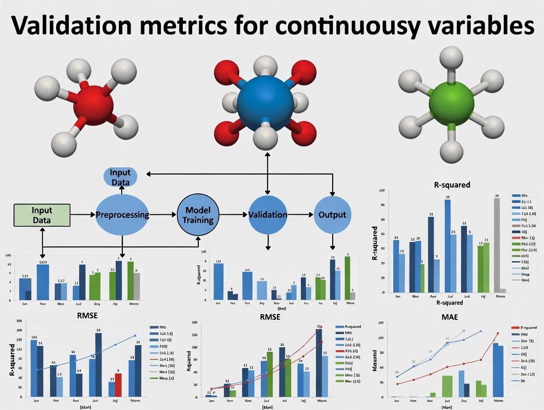
Key Validation Metrics for Continuous Variables

For research involving continuous variables—such as biomarker concentrations, pharmacokinetic parameters, or physiological measurements—specific validation metrics are employed to quantify model performance against ground truth data. These metrics provide standardized, quantitative assessments of how well a model's predictions align with observed values.

The following table summarizes the core validation metrics used for continuous variable models in scientific research:

Table 1: Key Validation Metrics for Models with Continuous Outputs

Metric	Mathematical Formula	Interpretation	Use Case in Drug Development
Mean Absolute Error (MAE)	$MAE=\frac{1}{n}{\sum }_{i=1}^n$	yi-y^i		Average magnitude of prediction errors (same units as variable). Lower values indicate better performance.	Predicting patient-specific drug dosage levels where the cost of error is linear and consistent.
Mean Squared Error (MSE)	$MSE=\frac{1}{n}{\sum }_{i=1}^n(y_i-{\hat{y}}_i{)}^2$	Average of squared errors. Penalizes larger errors more heavily than MAE.	Validating pharmacokinetic models where large prediction errors (e.g., in peak plasma concentration) are disproportionately dangerous.
Root Mean Squared Error (RMSE)	$RMSE=\sqrt{MSE}$	Square root of MSE. Restores units to the original scale.	Evaluating prognostic models for tumor size reduction; provides error in clinically interpretable units (e.g., mm).
Coefficient of Determination (R²)	$R^2=1-\frac{{\sum }_i(y_i-{\hat{y}}_i{)}^2}{{\sum }_i(y_i-\overline{y}{)}^2}$	Proportion of variance in the dependent variable that is predictable from the independent variables.	Assessing a model predicting continuous clinical trial endpoints; indicates how well the model explains variability in patient response.

Each metric offers a distinct perspective on model performance. While MAE provides an easily interpretable average error, MSE and RMSE are more sensitive to outliers and large errors, which is critical in safety-sensitive applications [28]. R² is particularly valuable for understanding the explanatory power of a model beyond mere prediction error, indicating how well the model captures the underlying variance in the biological system [28].

The Critical Link Between Validation Metrics and Data Quality

Validation metrics and data quality dimensions exist in a symbiotic relationship. The reliability of any validation metric is fundamentally constrained by the quality of the data used to compute it. This relationship can be visualized as a workflow where data quality serves as the foundation for meaningful validation.

Diagram 1: Workflow from data quality to trusted insights.

The following table details how specific data quality dimensions directly impact the integrity and reliability of validation metrics:

Table 2: How Data Quality Dimensions Impact Validation Metrics

Data Quality Dimension	Impact on Validation Metrics	Example in Research Context
Accuracy [29] [30]	Inaccurate ground truth data creates a false baseline, rendering all validation metrics meaningless and providing a misleading sense of model performance.	If true patient blood pressure measurements are systematically miscalibrated, a model's low MAE would be an artifact of measurement error, not predictive accuracy.
Completeness [30] [32]	Missing data points in the test set bias validation metrics. The calculated error may not be representative of the model's true performance across the entire data distribution.	A model predicting drug efficacy trained and tested on a dataset missing outcomes for elderly patients will yield unreliable R² values for the overall population.
Consistency [29] [33]	Inconsistent data formats or units (e.g., mg vs µg) introduce artificial errors, inflating metrics like MSE and RMSE without reflecting the model's actual predictive capability.	Merging lab data from multiple clinical sites that use different units for a biomarker without standardization will artificially inflate the RMSE of a prognostic model.
Validity [30] [34]	Data that violates business rules (e.g., negative values for a physical quantity) causes model failures and computational errors during validation.	A physiological model expecting a positive heart rate will fail or produce garbage outputs if the validation set contains negative values, preventing metric calculation.
Timeliness [35] [33]	Using outdated data for validation fails to assess how the model performs on current, relevant data, leading to metrics that don't reflect real-world usability.	Validating a model for predicting seasonal disease outbreaks with data from several years ago may show good MAE but fail to capture recent changes in pathogen strains.

This interplay necessitates a "multi-metric, context-aware evaluation" [27] that considers both the statistical performance of the model and the data quality that underpins it. For instance, a surprisingly low MSE should prompt an investigation into data accuracy and consistency, not just be taken as a sign of a good model.

Experimental Protocols for Robust Model Validation

Implementing a rigorous, standardized protocol for model validation is essential for generating credible, reproducible results. The following workflow outlines a comprehensive methodology that integrates data quality checks directly into the validation process.

Diagram 2: End-to-end model validation protocol.

Phase 1: Data Preparation and Quality Control

• Dataset Partitioning: Split the source data into three distinct sets: training (e.g., 70%), validation (e.g., 15%), and a hold-out test set (e.g., 15%). The hold-out test set must remain completely untouched until the final validation phase [28].
• Data Quality Profiling: Use automated data profiling tools [30] or custom scripts to assess the quality of each dataset against the core dimensions:
  • Completeness: Calculate the percentage of missing values for each critical field. Establish a threshold (e.g., >5% missingness may require imputation or exclusion) [35].
  • Accuracy and Validity: Perform range validation [34] to ensure continuous variables fall within physiologically or clinically plausible limits (e.g., human body temperature between 35°C and 42°C). Apply format validation to categorical variables and identifiers.
  • Consistency: Check for unit uniformity and consistent data formats across all records [32].
• Data Remediation: Based on the profiling results, apply techniques like imputation for missing data (with careful documentation of the method) or correction of invalid values. Any remediation applied to the training set must be applied identically to the validation and test sets.

Phase 2: Model Training and Validation

• Model Training: Train the model using only the training dataset.
• Hyperparameter Tuning: Use the validation set to tune model hyperparameters. This prevents information from the test set leaking into the model development process.
• Final Validation: Execute the final, tuned model on the pristine hold-out test set to generate predictions. This step is crucial for obtaining an unbiased estimate of model performance on new, unseen data [28].

Phase 3: Metric Calculation and Analysis

• Compute Validation Metrics: Calculate the key metrics outlined in Table 1 (MAE, MSE, RMSE, R²) by comparing the model's predictions on the test set to the ground truth values.
• Uncertainty Quantification (UQ): Go beyond point estimates by quantifying uncertainty in the model's predictions. This can involve calculating confidence intervals for the validation metrics or using Bayesian methods to provide probabilistic predictions [31]. UQ is essential for communicating the reliability of model outputs in clinical decision-making.
• Continuous Validation: For models deployed in production, establish a continuous model validation cadence [36]. This involves periodically re-validating the model on newly acquired data to detect and alert on "data drift," where the statistical properties of the incoming data change over time, degrading model performance.

To implement the protocols and metrics described, researchers require a suite of methodological "reagents" – the essential tools, software, and conceptual frameworks that enable robust validation and data quality management.

Table 3: Essential Research Reagent Solutions for Validation and Data Quality

Tool Category	Specific Examples & Functions	Application in Validation & Data Quality
Statistical & Programming Frameworks	R (caret, tidyverse), Python (scikit-learn, pandas, NumPy, SciPy)	Provide libraries for calculating all key validation metrics (MAE, MSE, R²), statistical analysis, and data manipulation. Essential for implementing custom validation workflows.
Data Profiling & Quality Tools	OvalEdge [30], Monte Carlo [33], custom SQL/Python scripts	Automate the assessment of data quality dimensions like completeness (missing values), uniqueness (duplicates), and validity. Generate reports to baseline data quality before model development.
Validation-Specific Software	Snorkel Flow [36], MLflow	Support continuous model validation [36], track experiment metrics, and manage model versions. Crucial for maintaining model reliability post-deployment in dynamic environments.
Uncertainty Quantification (UQ) Libraries	Python (PyMC3, TensorFlow Probability, UQpy)	Implement Bayesian methods and other statistical techniques to quantify epistemic (model) and aleatoric (data) uncertainty [31], providing confidence bounds for predictions.
Data Validation Frameworks	Great Expectations, Amazon Deequ, JSON Schema [34]	Define and enforce "constraint validation" [34] rules (e.g., value ranges, allowed categories) programmatically, ensuring data validity and consistency throughout the data pipeline.

The path to reliable, clinically relevant insights in drug development and precision medicine is a function of both sophisticated models and high-quality data. Key validation metrics like MAE, RMSE, and R² provide the quantitative rigor needed to assess model performance, while data quality dimensions—accuracy, completeness, consistency, validity, and timeliness—form the essential foundation upon which these metrics can be trusted. As the field advances with technologies like digital twins for precision medicine, the integrated framework of Verification, Validation, and Uncertainty Quantification (VVUQ) highlighted by the National Academies [31] becomes increasingly critical. By adopting the experimental protocols and tools outlined in this guide, researchers can ensure their work on continuous variables is not only statistically sound but also built upon a trustworthy data base, ultimately accelerating the translation of data-driven models into safe and effective patient therapies.

The validation landscape in regulated industries, particularly pharmaceuticals and medical devices, is undergoing a fundamental transformation. By 2025, digital validation has moved from an emerging trend to a mainstream practice, with 58% of organizations now using digital validation systems—a significant increase from just 30% the previous year [37]. This shift is driven by the need for greater efficiency, enhanced data integrity, and sustained audit readiness in an increasingly complex regulatory environment. The transformation extends beyond mere technology adoption to encompass new methodologies, skill requirements, and strategic approaches that are reshaping how organizations approach compliance and quality assurance.

This guide examines the current state of digital validation practices, comparing traditional versus modern approaches, analyzing implementation challenges, and exploring emerging technologies. For researchers and drug development professionals, understanding these trends is crucial for building robust validation frameworks that meet both current and future regulatory expectations while accelerating product development timelines.

Current State Analysis: Digital Validation Adoption and ROI

The 2025 validation landscape demonstrates significant digital maturation, yet reveals critical implementation gaps that affect return on investment (ROI) and operational efficiency.

Table 1: Digital Validation Adoption Metrics (2025)

Metric	Value	Significance
Organizations using digital validation systems	58%	28% increase since 2024, indicating rapid sector-wide transformation [37]
Organizations meeting/exceeding ROI expectations	63%	Majority of adopters achieving tangible financial benefits [38]
Digital systems integrated with other tools	13%	Significant integration gap limiting potential value [37]
Teams reporting workload increases	66%	Persistent resource constraints despite technology adoption [38]
Organizations outsourcing validation work	70%	Strategic reliance on external expertise [39]

Digital Validation ROI and Performance Metrics

Recent industry data demonstrates that digital validation is delivering measurable value. According to the 2025 State of Validation Report, 98% of respondents indicate their digital validation systems met, exceeded, or were on track to meet expectations, with only 2% reporting significant disappointment in ROI [37]. Organizations implementing comprehensive digital validation frameworks report performance improvements including:

• 50-70% faster cycle times for validation protocols [40] [38]
• Near-zero audit deviations due to traceable documentation [40]
• Up to 90% reduction in labor costs for documentation management [40]

However, the full potential of digital validation remains unrealized for many organizations due to integration challenges. Nearly 70% of organizations report their digital validation systems operate in silos, disconnected from project management, data analytics, or Turn Over Package (TOP) systems [37]. This integration gap creates unnecessary manual effort and limits visibility across the validation lifecycle.

Comparative Analysis: Traditional vs. Digital Validation Models

The transition from document-centric to data-centric validation represents a paradigm shift in how regulated industries approach compliance.

Table 2: Document-Centric vs. Data-Centric Validation Models

Aspect	Document-Centric Model	Data-Centric Model
Primary Artifact	PDF/Word Documents	Structured Data Objects [38]
Change Management	Manual Version Control	Git-like Branching/Merging [38]
Audit Readiness	Weeks of Preparation	Real-Time Dashboard Access [38]
Traceability	Manual Matrix Maintenance	Automated API-Driven Links [38]
AI Compatibility	Limited (OCR-Dependent)	Native Integration [38]

The Data-Centric Validation Framework

Progressive organizations are moving beyond "paper-on-glass" approaches—where digital systems simply replicate paper-based workflows—toward truly data-centric validation models. This transition enables four critical capabilities:

• Unified Data Layer Architecture: Replacing fragmented document-centric models with centralized repositories enables real-time traceability and automated compliance with ALCOA++ principles [38].

• Dynamic Protocol Generation: AI-driven systems can analyze historical protocols and regulatory guidelines to auto-generate context-aware test scripts, though regulatory acceptance remains a barrier [38].

• Continuous Process Verification (CPV): IoT sensors and real-time analytics enable proactive quality management by feeding live data from manufacturing equipment into validation platforms [38].

• Validation as Code: Representing validation requirements as machine-executable code enables automated regression testing during system updates and Git-like version control for protocols [38].

Figure 1: Evolution from traditional to data-centric validation approaches, highlighting key characteristics and limitations at each stage.

Workforce and Resource Challenges in Digital Validation

Despite technological advancements, human factors remain significant challenges in digital validation implementation.

Table 3: 2025 Validation Workforce Composition and Challenges

Workforce Metric	Value	Implication
Teams with 1-3 dedicated staff	39%	Lean resourcing constraining digital transformation initiatives [39]
Professionals with 6-15 years experience	42%	Mid-career dominance creating experience gaps as senior experts retire [38]
Organizations citing resistance to change	45%	Cultural and organizational barriers outweigh technical challenges [37]
Teams reporting complexity challenges	49%	Validation complexity remains primary implementation hurdle [37]

Strategic Responses to Workforce Challenges

Forward-thinking organizations are addressing these workforce challenges through several key strategies:

• Targeted Outsourcing: With 70% of firms now outsourcing part of their validation workload, organizations are building hybrid internal-external team models that balance cost control with specialized expertise [39].

• Digital Champions Programs: Identifying and empowering enthusiastic employees within each department to act as local experts and advocates for digital validation tools, providing peer support and driving adoption [41].

• Cross-Functional Training: Developing data fluency across validation, quality, and technical teams to bridge the gap between domain expertise and digital implementation capabilities [38].

The 2025 State of Validation Report notes that the most commonly reported implementation challenges aren't technical—they're cultural and organizational, with 45% of organizations struggling with resistance to change and 38% having trouble ensuring user adoption [37].

AI and Emerging Technologies in Validation

Artificial intelligence adoption in validation remains in early stages but shows significant potential for transforming traditional approaches.

Table 4: AI Adoption in Validation (2025)

AI Application	Adoption Rate	Reported Impact
Protocol Generation	12%	40% faster drafting through NLP analysis of historical protocols [38]
Risk Assessment Automation	9%	30% reduction in deviations through predictive risk modeling [38]
Predictive Analytics	5%	25% improvement in audit readiness through pattern recognition [38]
Anomaly Detection	7%	Early identification of validation drift and non-conformance patterns [40]

AI Implementation Framework for Validation

While AI adoption rates remain modest, leading organizations are building foundational capabilities for AI integration:

• Data Quality Foundation: AI effectiveness in validation depends heavily on underlying data quality, with metrics including freshness (how current the data is), bias (representation balance), and completeness (absence of critical gaps) being essential prerequisites [42].

• Computer Software Assurance (CSA) Adoption: Despite regulatory encouragement, only 16% of organizations have fully adopted CSA, which provides a risk-based approach to software validation that aligns well with AI-assisted methodologies [39].

• Staged Implementation Approach: Successful organizations typically begin AI integration with low-risk applications such as document review and compliance checking before progressing to higher-impact areas like predictive analytics and automated protocol generation [38].

According to industry analysis, "AI is something to consider for the future rather than immediate implementation, as we still need to fully understand how it functions. There are substantial concerns regarding the validation of AI systems that the industry must address" [38].

Global Regulatory Initiatives and Standards

Digital transformation in validation is occurring within an evolving global regulatory framework that increasingly emphasizes data integrity and digital compliance.

China's Pharmaceutical Digitization Initiative

China's recent "Pharmaceutical Industry Digital Transformation Implementation Plan (2025-2030)" outlines ambitious digital transformation goals, including:

• Developing 30+ pharmaceutical industry digital technology standards by 2027 [43]
• Creating 100+ digital technology application scenarios covering R&D, production, and quality management [43]
• Establishing 10+ pharmaceutical large model innovation platforms and digital technology application verification platforms [43]
• Achieving comprehensive digital transformation coverage for scale pharmaceutical enterprises by 2030 [43]

This initiative emphasizes computerized system validation (CSV) guidelines specifically addressing process control, quality control, and material management systems [43].

Integrated Validation Framework Implementation

The AAA Framework (Audit, Automate, Accelerate) exemplifies the integrated approach organizations are taking to digital validation:

• Audit Phase: Comprehensive assessment of processes, data readiness, and regulatory conformance to establish a quantified baseline for digital validation implementation [40].

• Automate Phase: Workflow redesign incorporating AI agents, digital twins, and human-in-the-loop validation cycles with continuous documentation trails [40].

• Accelerate Phase: Implementation of governance dashboards, feedback loops, and reusable blueprints to scale validated systems across organizations [40].

Organizations implementing such frameworks report moving from reactive compliance to building "always-ready" systems that maintain continuous audit readiness through proactive risk mitigation and self-correcting workflows [38].

Essential Research Reagent Solutions for Digital Validation

Implementing effective digital validation requires specific technological components and methodological approaches.

Table 5: Digital Validation Research Reagent Solutions

Solution Category	Specific Technologies	Function in Validation Research
Digital Validation Platforms	Kneat, ValGenesis, SAS	Electronic management of validation lifecycle, protocol execution, and deviation management [37]
Data Integrity Tools	Blockchain-based audit trails, Electronic signatures, Version control systems	Ensure ALCOA++ compliance, prevent data tampering, maintain complete revision history [43]
Integration Frameworks	RESTful APIs, ESB, Middleware	Connect validation systems with manufacturing equipment, LIMS, and ERP systems [37]
Analytics and Monitoring	Process mining, Statistical process control, Real-time dashboards	Continuous monitoring of validation parameters, early anomaly detection [38]
AI/ML Research Tools	Natural Language Processing, Computer vision, Predictive algorithms	Automated document review, visual inspection verification, risk prediction [38]

The digital transformation of validation practices in 2025 represents both a challenge and opportunity for researchers and drug development professionals. Organizations that successfully navigate this transition are those treating validation as a strategic capability rather than a compliance obligation. The most successful organizations embed validation and governance into their operating models from the outset, with high performers treating "validation as a design layer, not a delay" [40].

As global regulatory frameworks evolve to accommodate digital approaches, professionals who develop expertise in data-centric validation, AI-assisted compliance, and integrated quality systems will be well-positioned to lead in an increasingly digital pharmaceutical landscape. The organizations that thrive will be those that view digital validation not as a cost center, but as a strategic asset capable of accelerating development timelines while enhancing product quality and patient safety.

From Theory to Practice: Essential Methods and Real-World Applications

In the realm of research, particularly in fields such as drug development and clinical studies, the validation of continuous variables against meaningful benchmarks is paramount. The t-test family provides foundational statistical methods for comparing means when population standard deviations are unknown, making these tests particularly valuable for analyzing sample data from larger populations [44] [45]. These parametric tests enable researchers to determine whether observed differences in continuous data—such as blood pressure measurements, laboratory values, or clinical assessment scores—represent statistically significant effects or merely random variation [2].

T-tests occupy a crucial position in hypothesis testing for continuous data, serving as a bridge between descriptive statistics and more complex analytical methods. Their relative simplicity, computational efficiency, and interpretability have made them a staple in research protocols across scientific disciplines [46]. For researchers and drug development professionals, understanding the proper application, assumptions, and limitations of each t-test type is essential for designing robust studies and drawing valid conclusions from experimental data.

Fundamental Concepts and Assumptions

Core Principles of T-Testing

All t-tests share fundamental principles despite their different applications. At their core, t-tests evaluate whether the difference between group means is statistically significant by calculating a t-statistic, which represents the ratio of the difference between means to the variability within the groups [47]. This test statistic is then compared to a critical value from the t-distribution—a probability distribution that accounts for the additional uncertainty introduced when estimating population parameters from sample data [45].

The t-distribution resembles the normal distribution but has heavier tails, especially with smaller sample sizes. As sample sizes increase, the t-distribution approaches the normal distribution [48]. This relationship makes t-tests particularly valuable for small samples (typically n < 30), where the z-test would be inappropriate [45] [46].

Key Assumptions for Parametric T-Tests

For t-tests to yield valid results, several assumptions must be met:

• Continuous data: The dependent variable should be measured on an interval or ratio scale [44] [2].
• Independence of observations: Data points must not influence each other, except in the case of paired designs where the pairing is the focus [47] [46].
• Approximate normality: The data should follow a normal distribution, though t-tests are reasonably robust to minor violations of this assumption, especially with larger sample sizes (n > 30) due to the Central Limit Theorem [2] [48].
• Homogeneity of variance: For independent samples t-tests, the variances in both groups should be approximately equal [44] [47].

When these assumptions are severely violated, researchers may need to consider non-parametric alternatives such as the Wilcoxon Signed-Rank test or data transformation techniques [47] [2].

One-Tailed vs. Two-Tailed Tests

An important consideration in t-test selection is whether to use a one-tailed or two-tailed test:

• Two-tailed tests examine whether means are different in either direction and are appropriate when research questions simply ask if a difference exists [44] [45].
• One-tailed tests examine whether one mean is specifically greater or less than another and should only be used when there is a strong prior directional hypothesis before data collection [44] [46].

Table 1: Comparison of One-Tailed and Two-Tailed Tests

Feature	One-Tailed Test	Two-Tailed Test
Direction of Interest	Specific direction	Either direction
Alternative Hypothesis	Specifies direction	No direction specified
Critical Region	One tail	Both tails
Statistical Power	Higher for specified direction	Lower, but detects effects in both directions
When to Use	Strong prior direction belief	Any difference is of interest

The t-test family comprises three primary tests, each designed for specific research scenarios and data structures. Understanding the distinctions between these tests is crucial for selecting the appropriate analytical approach.

One-Sample T-Test

The one-sample t-test compares the mean of a single group to a known or hypothesized population value [44] [49]. This test answers the question: "Does our sample come from a population with a specific mean?"

Independent Samples T-Test

Also known as the two-sample t-test or unpaired t-test, the independent samples t-test compares means between two unrelated groups [44] [47]. This test determines whether there is a statistically significant difference between the means of two independent groups.

Paired T-Test

The paired t-test (also called dependent samples t-test) compares means between two related groups [44] [50]. This test is appropriate when measurements are naturally paired or matched, such as pre-test/post-test designs or matched case-control studies.

Table 2: Comparison of T-Test Types

Test Type	Number of Variables	Purpose	Example Research Question
One-Sample	One continuous variable	Decide if population mean equals a specific value	Is the mean heart rate of a group equal to 65?
Independent Samples	One continuous and one categorical variable (2 groups)	Decide if population means for two independent groups are equal	Do mean heart rates differ between men and women?
Paired Samples	Two continuous measurements from matched pairs	Decide if mean difference between paired measurements is zero	Is there a difference in blood pressure before and after treatment?

Decision Workflow for T-Test Selection

Selecting the appropriate t-test requires careful consideration of your research design, data structure, and hypothesis. The following diagram illustrates a systematic approach to t-test selection:

Figure 1: T-Test Selection Workflow

One-Sample T-Test

Methodology and Applications

The one-sample t-test evaluates whether the mean of a single sample differs significantly from a specified value [44]. This test is particularly useful in quality control, method validation, and when comparing study results to established standards.

The test statistic for the one-sample t-test is calculated as:

[ t = \frac{\bar{x} - \mu_0}{s/\sqrt{n}} ]

Where (\bar{x}) is the sample mean, (\mu_0) is the hypothesized population mean, (s) is the sample standard deviation, and (n) is the sample size [2] [48].

Experimental Protocol

Research Scenario: A pharmaceutical company wants to validate that the average dissolution time of a new generic drug formulation meets the standard reference value of 30 minutes established by the regulatory agency.

Step-by-Step Protocol:

• Define hypotheses:

  • Null hypothesis (H₀): The mean dissolution time equals 30 minutes ((\mu = 30))
  • Alternative hypothesis (H₁): The mean dissolution time differs from 30 minutes ((\mu \ne 30))

• Set significance level: Typically α = 0.05 [2]

• Collect data: Randomly select 25 tablets from production and measure dissolution time for each

• Check assumptions:

  • Independence: Ensure tablets are randomly selected
  • Normality: Assess using histogram, Q-Q plot, or Shapiro-Wilk test [2]

• Calculate test statistic using the formula above

• Determine critical value from t-distribution with n-1 degrees of freedom

• Compare test statistic to critical value and make decision regarding H₀

• Interpret results in context of research question

Real-World Application Example

In manufacturing, an engineer might use a one-sample t-test to determine if products created using a new process have a different mean battery life from the current standard of 100 hours [51]. After testing 50 products, if the analysis shows a statistically significant difference, this would provide evidence that the new process affects battery life.

Independent Samples T-Test

Methodology and Applications

The independent samples t-test (also called unpaired t-test) compares means between two unrelated groups [47] [48]. This test is widely used in randomized controlled trials, A/B testing, and any research design with two independent experimental groups.

The test statistic for the independent samples t-test is calculated as:

[ t = \frac{\bar{x1} - \bar{x2}}{sp \sqrt{\frac{1}{n1} + \frac{1}{n_2}}} ]

Where (\bar{x1}) and (\bar{x2}) are the sample means, (n1) and (n2) are the sample sizes, and (s_p) is the pooled standard deviation [2].

Experimental Protocol

Research Scenario: A research team is comparing the efficacy of two different diets (A and B) on weight loss in a randomized controlled trial.

Step-by-Step Protocol:

• Define hypotheses:

  • H₀: Mean weight loss is the same for both diets ((\mu1 = \mu2))
  • H₁: Mean weight loss differs between diets ((\mu1 \ne \mu2))

• Set significance level: α = 0.05

• Design study: Randomly assign 20 subjects to Diet A and 20 subjects to Diet B [51]

• Collect data: Measure weight loss for each subject after one month

• Check assumptions:

  • Independence: Ensure random assignment and no communication between groups
  • Normality: Check distribution of weight loss in each group
  • Homogeneity of variance: Assess using Levene's test or similar method [48]

• Calculate test statistic and degrees of freedom

• Determine critical value from t-distribution

• Compare test statistic to critical value and make decision

• Calculate confidence interval for the mean difference

• Interpret results in context of clinical significance

Experimental Design Visualization

The following diagram illustrates the typical experimental design for an independent samples t-test:

Figure 2: Independent Samples T-Test Experimental Design

Real-World Application Example

In education research, a professor might use an independent samples t-test to compare exam scores between students who used two different studying techniques [51]. By randomly assigning students to each technique and ensuring no interaction between groups, the professor can attribute any statistically significant difference in means to the studying technique rather than confounding variables.

Paired Samples T-Test

Methodology and Applications

The paired samples t-test (also called dependent samples t-test) compares means between two related measurements [50]. This test is appropriate for pre-test/post-test designs, matched case-control studies, repeated measures, or any scenario where observations naturally form pairs.

The test statistic for the paired samples t-test is calculated as:

[ t = \frac{\bar{d}}{s_d/\sqrt{n}} ]

Where (\bar{d}) is the mean of the differences between paired observations, (s_d) is the standard deviation of these differences, and (n) is the number of pairs [2] [50].

Experimental Protocol

Research Scenario: A clinical research team is evaluating the effectiveness of a new blood pressure medication by comparing patients' blood pressure before and after treatment.

Step-by-Step Protocol:

• Define hypotheses:

  • H₀: The mean difference in blood pressure is zero ((\mu_d = 0))
  • H₁: The mean difference in blood pressure is not zero ((\mu_d \ne 0))

• Set significance level: α = 0.05

• Design study: Recruit 15 patients with hypertension and measure blood pressure before and after a 4-week treatment period [51]

• Collect data: Record paired measurements for each subject

• Check assumptions:

  • Independence: Differences between pairs should be independent
  • Normality: The distribution of differences should be approximately normal [50]

• Calculate differences for each pair of observations

• Compute mean and standard deviation of the differences

• Calculate test statistic using the formula above

• Determine critical value from t-distribution with n-1 degrees of freedom

• Compare test statistic to critical value

• Interpret results including both statistical and clinical significance

Experimental Design Visualization

The following diagram illustrates the typical experimental design for a paired samples t-test:

Figure 3: Paired Samples T-Test Experimental Design

Real-World Application Example

In pharmaceutical research, a paired t-test might be used to evaluate a new fuel treatment by measuring miles per gallon for 11 cars with and without the treatment [51]. Since each car serves as its own control, the paired design eliminates variability between different vehicles, providing a more powerful test for detecting the treatment effect.

Data Analysis and Interpretation

Comprehensive Comparison of T-Test Results

When reporting t-test results, researchers should include key elements that allow for proper interpretation and replication. The following table summarizes essential components for each t-test type:

Table 3: Key Reporting Elements for Each T-Test Type

Test Element	One-Sample T-Test	Independent Samples	Paired Samples
Sample Size	n	n₁, n₂	n (number of pairs)
Mean(s)	Sample mean ((\bar{x}))	Group means ((\bar{x1}), (\bar{x2}))	Mean of differences ((\bar{d}))
Standard Deviation	Sample SD (s)	Group SDs (s₁, s₂) or pooled SD	SD of differences (s_d)
Test Statistic	t-value	t-value	t-value
Degrees of Freedom	n - 1	n₁ + n₂ - 2	n - 1
P-value	p-value	p-value	p-value
Confidence Interval	CI for population mean	CI for difference between means	CI for mean difference

Interpretation Guidelines

Proper interpretation of t-test results extends beyond statistical significance to consider practical importance:

• Statistical significance: If p < α, reject the null hypothesis and conclude there is a statistically significant difference [2]

• Effect size: Calculate measures such as Cohen's d to assess the magnitude of the effect, not just its statistical significance

• Confidence intervals: Examine the range of plausible values for the population parameter

• Practical significance: Consider whether the observed difference is meaningful in the real-world context

• Assumption checks: Report any violations of assumptions and how they were addressed

For example, in a paired t-test analysis of exam scores, researchers found a mean difference of 1.31 with a t-statistic of 0.75 and p-value > 0.05, leading to the conclusion that there was no statistically significant difference between the exams [50].

Research Reagent Solutions and Materials

The following table outlines essential materials and methodological components for implementing t-test analyses in research contexts:

Table 4: Essential Research Materials for T-Test Applications

Item Category	Specific Examples	Research Function
Statistical Software	R, SPSS, JMP, Prism, GraphPad	Perform t-test calculations, assumption checks, and visualization [47] [50]
Data Collection Tools	Electronic data capture systems, Laboratory information systems	Ensure accurate, reliable measurement of continuous variables [2]
Normality Testing	Shapiro-Wilk test, Kolmogorov-Smirnov test, Q-Q plots	Verify normality assumption required for parametric testing [2] [50]
Sample Size Calculators	Power analysis software, Online calculators	Determine adequate sample size to achieve sufficient statistical power
Randomization Tools	Random number generators, Allocation software	Ensure unbiased group assignment for independent designs [51]

Advanced Considerations and Alternatives

Handling Assumption Violations

When t-test assumptions are violated, researchers have several options:

• Non-normal data: Consider data transformations (log, square root) or non-parametric alternatives like Mann-Whitney U test (independent samples) or Wilcoxon signed-rank test (paired samples) [2]

• Unequal variances: Use Welch's t-test, which does not assume equal variances and automatically adjusts degrees of freedom [2] [48]

• Small sample sizes: Focus on effect sizes and confidence intervals rather than relying solely on p-values

• Outliers: Investigate whether outliers represent errors or genuine observations, and consider robust statistical methods if appropriate

When to Use Alternatives to T-Tests

While t-tests are versatile, certain research scenarios require alternative approaches:

• Comparing more than two groups: Use Analysis of Variance (ANOVA) followed by post-hoc tests for detailed group comparisons [44] [2]

• Repeated measurements over time: Consider repeated measures ANOVA or mixed-effects models

• Non-continuous data: Use chi-square tests (categorical data) or non-parametric alternatives

• Complex relationships: Consider regression models that can accommodate multiple predictors and control for confounding variables

The choice between t-tests and alternative methods should be guided by research questions, study design, and data characteristics rather than statistical convenience.

The t-test family provides fundamental tools for comparing means in research involving continuous variables. Proper application of these tests requires understanding their distinct purposes, assumptions, and interpretation frameworks. The one-sample t-test compares a single mean to a reference value, the independent samples t-test compares means between unrelated groups, and the paired samples t-test compares means within related observations.

In drug development and scientific research, selecting the appropriate t-test ensures valid conclusions from experimental data. By following structured protocols, checking assumptions, and considering both statistical and practical significance, researchers can robustly validate their hypotheses and contribute meaningful evidence to their fields. As research questions grow more complex, t-tests remain essential components in the analytical toolkit, often serving as building blocks for more sophisticated statistical models while maintaining their utility for straightforward group comparisons.

In the realm of research involving continuous variables, the comparison of means across different experimental groups constitutes a fundamental analytical task. While the t-test provides a well-established method for comparing means between two groups, many research scenarios in drug development and biological sciences require simultaneous comparison across three or more experimental conditions [52]. This common research challenge creates a statistical dilemma: conducting multiple pairwise t-tests dramatically increases the probability of false positive findings (Type I errors) due to the problem of multiple comparisons [53].

Analysis of Variance (ANOVA) represents a powerful extension of the t-test principle that addresses this limitation by enabling researchers to test whether there are statistically significant differences among three or more group means while maintaining the overall Type I error rate at the chosen significance level [54]. This methodological advancement is particularly crucial in validation metrics for continuous variables research, where maintaining statistical integrity while comparing multiple interventions, treatments, or conditions is paramount. The fundamental question ANOVA addresses is whether the observed differences between group means are greater than would be expected due to random sampling variation alone [55].

Fundamental Principles: From T-Test to ANOVA

Conceptual Foundation

Both the t-test and ANOVA are parametric tests that compare means under the assumption that the dependent variable is continuous and approximately normally distributed [52]. While the t-test evaluates the difference between two means by examining the ratio of the mean difference to the standard error, ANOVA assesses whether the variance between group means is substantially larger than the variance within groups [56]. The key distinction lies in their scope of application: t-tests are limited to two-group comparisons, whereas ANOVA can handle multiple groups simultaneously [57].

The null hypothesis (H₀) for ANOVA states that all group means are equal (μ₁ = μ₂ = μ₃ = ... = μₖ), while the alternative hypothesis (H₁) posits that at least one group mean differs significantly from the others [58]. This global test provides protection against the inflation of Type I errors that occurs when conducting multiple t-tests without appropriate correction [53]. When the overall ANOVA result is statistically significant, post-hoc tests are required to identify which specific groups differ from each other [54].

Statistical Mechanics

ANOVA operates by partitioning the total variance in the data into two components: variance between groups (explained by the treatment or grouping factor) and variance within groups (unexplained random error) [55]. The test statistic for ANOVA is the F-ratio, calculated as the ratio of between-group variance to within-group variance [53]:

F = Variance Between Groups / Variance Within Groups

A larger F-value indicates that between-group differences are substantial relative to the random variation within groups, providing evidence against the null hypothesis [54]. The associated p-value indicates the probability of obtaining the observed results (or more extreme results) if the null hypothesis were true [52].

Table 1: Key Differences Between T-Test and ANOVA

Feature	T-Test	ANOVA
Purpose	Compares means between two groups	Compares means across three or more groups
Number of Groups	Two groups only	Three or more groups
Hypothesis Tested	H₀: μ₁ = μ₂	H₀: μ₁ = μ₂ = μ₃ = ... = μₖ
Test Statistic	t-statistic	F-statistic
Post-hoc Testing	Not required	Required after significant overall test
Experimental Designs	Simple comparisons	Complex multi-group designs

Methodological Framework

Core Assumptions

The validity of ANOVA results depends on several statistical assumptions that must be verified before conducting the analysis [54] [58]:

• Independence of Observations: Each data point must be independent of all other data points. This assumption is typically addressed through proper experimental design, including random sampling and assignment [58].
• Normality: The dependent variable should be approximately normally distributed within each group. While ANOVA is relatively robust to minor violations of this assumption, especially with larger sample sizes, extreme departures from normality may affect the validity of results [54].
• Homogeneity of Variance (Homoscedasticity): The variance within each group should be roughly equal across all groups. This assumption can be tested using Levene's test or the Brown-Forsythe test [58].

Violations of these assumptions may require data transformation or the use of non-parametric alternatives such as the Kruskal-Wallis test [54]. The independence assumption is particularly critical, as violations can seriously compromise the validity of ANOVA results [58].

Types of ANOVA Designs

Several ANOVA designs accommodate different experimental structures:

• One-Way ANOVA: Used when comparing groups defined by a single categorical independent variable [52]. For example, comparing the effects of different dosage levels of a drug (low, medium, high) on a continuous outcome measure [54].
• Two-Way ANOVA: Extends the analysis to include two independent variables and their potential interaction effects [54]. This design allows researchers to examine how two different factors simultaneously influence the dependent variable and whether these factors interact [58].
• Repeated Measures ANOVA: Appropriate when the same subjects are measured under different conditions or across multiple time points [54]. This design accounts for the correlation between measurements from the same source, increasing statistical power [52].

Table 2: ANOVA Designs and Their Applications

ANOVA Type	Factors	Interaction Tested	Common Applications
One-Way ANOVA	One independent variable	No	Comparing multiple treatments or conditions
Two-Way ANOVA	Two independent variables	Yes	Examining main effects and interactions between two factors
Repeated Measures	One within-subjects factor	Possible with additional factors	Longitudinal studies, pre-post interventions

Experimental Protocols and Applications

Detailed Methodology: One-Way ANOVA Protocol

The implementation of one-way ANOVA follows a structured analytical process. Consider a preclinical study investigating the effects of THC on locomotor activity in mice across four dosage groups (VEH, 0.3, 1, and 3 mg/kg) [55]:

• Research Question Formulation: Determine whether different dosage levels of THC significantly affect locomotor activity in mice.
• Experimental Design: Randomly assign mice to four treatment groups with appropriate sample sizes in each group (e.g., 15, 9, 12, and 10 mice per group) [55].
• Data Collection: Measure locomotor activity as percentage of baseline activity for each mouse.
• Assumption Checking:
  • Test normality using Shapiro-Wilk test or visual inspection of Q-Q plots
  • Verify homogeneity of variances using Levene's test
  • Confirm independence through experimental design
• Model Fitting: Construct a linear model with percentofact (percentage of activity) as the dependent variable and group (dosage level) as the independent variable [55].
• ANOVA Execution: Calculate the F-statistic using statistical software.
• Result Interpretation: The example study yielded F(3,42) = 3.126, p = 0.0357, indicating statistically significant differences among the dosage groups [55].
• Post-hoc Analysis: Upon finding a significant result, conduct appropriate post-hoc tests (e.g., Tukey's HSD) to identify which specific group means differ.

Application in Drug Development Research

ANOVA finds extensive application in pharmaceutical research and development. The 2025 Alzheimer's disease drug development pipeline, for instance, includes 138 drugs across 182 clinical trials [59]. These trials naturally involve multiple treatment arms and dosage levels, creating ideal scenarios for ANOVA application. Biological disease-targeted therapies comprise 30% of the pipeline, while small molecule disease-targeted therapies account for 43% [59]. Comparing the efficacy of these different therapeutic approaches requires statistical methods capable of handling multiple group comparisons.

Biomarkers serve as primary outcomes in 27% of active AD trials [59], and these continuous biomarker measurements often need comparison across multiple treatment groups, dosage levels, or time points. ANOVA provides the methodological framework for these comparisons while controlling Type I error rates. Furthermore, with repurposed agents representing 33% of the pipeline agents [59], researchers frequently need to compare both novel and repurposed compounds simultaneously, another scenario where ANOVA excels.

Analytical Workflow and Output Interpretation

Comprehensive Analytical Process

The complete ANOVA workflow extends from experimental design through final interpretation:

Output Interpretation and Post-hoc Analysis

Interpreting ANOVA results requires understanding several key components. The ANOVA table typically includes degrees of freedom (df), sum of squares (SS), mean squares (MS), F-value, and p-value [55]. A significant p-value (typically < 0.05) indicates that at least one group mean differs significantly from the others but does not specify which groups differ [52].

When the overall ANOVA is significant, post-hoc tests control the experiment-wise error rate while identifying specific group differences [54]. Common post-hoc procedures include:

• Tukey's Honestly Significant Difference (HSD): Conservative test that controls the family-wise error rate for all pairwise comparisons [53]
• Bonferroni Correction: Divides the significance level by the number of comparisons [52]
• Dunnett's Test: Designed specifically for comparing multiple treatment groups to a single control group [54]

Table 3: ANOVA Output Interpretation Guide

ANOVA Output	Interpretation	Implication
F-value	Ratio of between-group to within-group variance	Larger values indicate greater group differences relative to within-group variability
p-value	Probability of observed results if null hypothesis true	p < 0.05 suggests statistically significant differences among groups
Degrees of Freedom	Number of independent pieces of information	df between = k-1; df within = N-k
Effect Size (η²)	Proportion of total variance attributable to group differences	Larger values indicate more practically significant effects

Advanced Applications and Extensions

Related Analytical Techniques

ANOVA serves as the foundation for several advanced statistical methods:

• ANCOVA (Analysis of Covariance): Extends ANOVA by incorporating continuous covariates into the model, allowing adjustment for potential confounding variables [52]. This is particularly valuable in observational studies where random assignment is not possible.
• MANOVA (Multivariate Analysis of Variance): Used when there are multiple correlated dependent variables, testing whether groups differ on a combination of these variables [58].
• Repeated Measures ANOVA: Appropriate for longitudinal studies where the same subjects are measured at multiple time points, accounting for within-subject correlations [52].

Practical Considerations for Researchers

Successful implementation of ANOVA requires attention to several practical considerations. Sample size significantly impacts statistical power, with small samples reducing the ability to detect genuine differences and very large samples potentially detecting trivial differences lacking practical importance [54]. Researchers should consider effect size measures alongside p-values to assess practical significance.

ANOVA is sensitive to outliers, which can disproportionately influence results, making careful data screening essential [54]. When assumptions are severely violated, alternatives such as data transformation, non-parametric tests, or robust statistical methods may be necessary. Modern statistical software packages (R, Python, SPSS, SAS) provide comprehensive ANOVA implementations with diagnostic capabilities to assess assumptions and model fit [54].

Table 4: Research Reagent Solutions for ANOVA Implementation

Tool Category	Specific Solutions	Function and Application
Statistical Software	R, Python, SPSS, SAS, JMP	Conduct ANOVA calculations, assumption checks, and post-hoc tests
Normality Testing	Shapiro-Wilk test, Kolmogorov-Smirnov test, Q-Q plots	Assess normality assumption for dependent variable within groups
Variance Homogeneity	Levene's test, Brown-Forsythe test	Verify equality of variances across groups
Post-hoc Analysis	Tukey's HSD, Bonferroni, Scheffé, Dunnett's tests	Identify specific group differences after significant ANOVA
Effect Size Measures	Eta-squared (η²), Partial Eta-squared, Omega-squared	Quantify practical significance of group differences
Data Visualization	Box plots, Mean plots, Interaction plots	Visualize group differences and patterns in data

ANOVA represents a fundamental advancement in statistical methodology that directly extends the t-test principle to complex research scenarios involving multiple group comparisons. Its ability to efficiently compare three or more groups while controlling Type I error rates makes it indispensable across scientific disciplines, particularly in drug development research where comparing multiple treatments, dosages, or experimental conditions is routine. The 2025 Alzheimer's disease drug development pipeline, with its 138 drugs across 182 clinical trials [59], exemplifies the critical need for robust multiple comparison methods.

Proper implementation of ANOVA requires careful attention to its underlying assumptions, appropriate experimental design, and thorough interpretation including post-hoc analysis when warranted. When applied correctly, ANOVA provides researchers with a powerful tool for making valid inferences about group differences in continuous variables, forming a cornerstone of quantitative analysis in scientific research and supporting evidence-based decision-making in pharmaceutical development and beyond.

Implementing Continuous Gage Repeatability and Reproducibility (GR&R) Studies in Manufacturing

For researchers, scientists, and drug development professionals, the integrity of continuous variable data is paramount. Continuous Gage Repeatability and Reproducibility (GR&R) studies serve as a critical statistical methodology within a broader validation metrics framework, providing objective evidence that measurement systems are capable of producing reliable data for critical quality attributes [60] [61]. In regulated manufacturing environments, particularly for pharmaceuticals and medical devices, this transcends mere best practice, becoming a compliance requirement under standards such as FDA 21 CFR Part 820 and ISO 13485 [60]. A measurement system itself encompasses the complete process of obtaining a measurement, including the gage (instrument), operators (appraisers), the parts or samples being measured, the documented procedures, and the environmental conditions [60] [61]. A continuous GR&R study quantitatively assesses this system, isolating and quantifying its inherent variability to ensure it is "fit-for-purpose" and that subsequent research conclusions and product quality decisions are based on trustworthy data [61] [62].

Core Principles and Regulatory Imperative

Deconstructing Measurement System Variation

The fundamental principle of GR&R is to partition the total observed variation in a process into its constituent parts: the variation from the actual parts themselves and the variation introduced by the measurement system [61]. The total variation is statistically represented as σ²Total = σ²Process + σ²Measurement [61]. The goal of a capable measurement system is to minimize σ²Measurement so that the observed data truly reflects the underlying process.

The "R&R" specifically refers to two core components of measurement system variation, which are visually conceptualized in the diagram below:

The statistical components of Gage R&R variation, where σ²MS = σ²Repeatability + σ²Reproducibility [61].

• Repeatability: This is the variation observed when one operator repeatedly measures the same characteristic on the same part using the same gage and method [60] [63]. It is often called "equipment variation" as it reflects the inherent precision of the gage itself [64]. Poor repeatability indicates instability in the measurement instrument [61] [65].
• Reproducibility: This is the variation in the average of measurements made by different operators while measuring the identical characteristic on the same part [60] [63]. This is often termed "appraiser variation" and can be influenced by differences in individual technique, skill, or interpretation of the measurement procedure [60] [65].

Compliance and Quality Risk Management

From a regulatory perspective, reliance on an unvalidated measurement system constitutes a significant quality risk. Regulatory frameworks like the FDA's 21 CFR Part 820.72 explicitly mandate that inspection and test equipment must be "suitable for its intended purposes and is capable of producing valid results" [60]. A GR&R study provides the documented, statistical evidence required to satisfy this requirement during audits. The risks of non-compliance include regulatory findings, warning letters, and in severe cases, product recalls if measurement error leads to the acceptance of non-conforming product (Type II error) or the erroneous rejection of good product (Type I error) [60]. Furthermore, in the context of risk management for medical devices (ISO 14971), an unvalidated measurement system is considered an unmitigated risk to patient safety [60].

Experimental Protocol for Continuous GR&R Studies

Executing a robust continuous GR&R study requires a structured protocol. The following workflow outlines the key phases from initial planning through to final analysis and system improvement.

A workflow for designing, executing, and analyzing a continuous GR&R study, synthesizing recommendations from multiple sources [61] [64] [66].

Prerequisites and Planning (Phase 1)

Before collecting data, foundational steps must be taken. First, address any known issues with the measurement system, such as equipment in need of calibration or outdated procedures, as running a GR&R on a knowingly flawed system wastes resources [66]. The study requires a minimum of 2-3 operators who regularly use the gage and 5-10 parts that are selected to represent the entire expected process variation, from low to high values [61] [64] [66]. This part selection is critical; if the samples are too similar, the study will not properly assess the system's ability to detect part-to-part differences [61].

Study Design and Execution (Phase 2)

The crossed study design is the most common for non-destructive testing, where each operator measures each part multiple times [63]. To minimize bias, the study should be conducted blindly and the order of measurement for all parts should be randomized for each operator and each trial (replicate) [67]. Each operator measures each part 2 to 3 times without seeing others' results or their own previous results for the same part [64]. This structured, randomized data collection is essential for generating unbiased data for the subsequent ANOVA analysis.

The Scientist's Toolkit: Essential Research Reagents and Materials

A successful GR&R study relies on more than just statistical theory. The following table details the key "research reagents" and materials required for execution.

Table 1: Essential Materials for a GR&R Study

Item	Function & Rationale
Measurement Instrument (Gage)	The device under validation. It must be calibrated and selected with a discrimination (resolution) fine enough to detect at least one-tenth of the total tolerance or process variation [61] [64].
Reference Parts / Samples	Physical artifacts representing the process range. They must be stable, homogeneous, and cover the full spectrum of the process variation to properly challenge the measurement system [60] [61].
Trained Operators (Appraisers)	Individuals who perform the measurements. They should represent the population of users and be trained on the standardized measurement procedure to minimize introduced variation [60] [61].
Standardized Measurement Procedure	A documented, detailed work instruction that specifies the precise method for taking the measurement, including sample preparation, environmental conditions, and data recording [60] [67].
Data Collection Sheet / Software	A structured medium for recording data. Using software like Minitab or DataLyzer Qualis 4.0 ensures proper randomization and facilitates accurate analysis [64] [65].

Analytical Methods and Metric Comparison

Statistical Analysis Using ANOVA

While the Average and Range method is a valid approximation, the Analysis of Variance (ANOVA) method is the preferred and more statistically robust approach for analyzing GR&R data [60] [64]. ANOVA does not assume the interaction between the operator and the part is negligible and can actually test for and quantify this interaction effect. This provides a more accurate and comprehensive breakdown of the variance components: repeatability, reproducibility (operator), operator*part interaction, and part-to-part variation [64].

Key Validation Metrics and Acceptance Criteria

The output of a GR&R analysis is interpreted using a standard set of metrics. The most common are presented as a percentage of the total study variation (%GRR) and as a percentage of the tolerance (%P/T). These metrics, along with their interpretation guidelines, are summarized in the table below. It is critical to note that these criteria can vary by industry, with the automotive industry (AIAG) guidelines being a common reference [64].

Table 2: Key GR&R Metrics and Interpretation Guidelines

Metric	Formula / Description	Interpretation (AIAG Guidelines)
%GRR(% Study Variation)	%GRR = (σMS / σTotal) × 100Where σMS is the combined Repeatability & Reproducibility standard deviation [61] [64].	< 10%: Acceptable10% - 30%: Marginal> 30%: Unacceptable [64]
%P/T(% Tolerance)	%P/T = (5.15 × σMS / Tolerance) × 100Where Tolerance = USL - LSL. The constant 5.15 covers 99% of the measurement variation [61] [64].	< 10%: Acceptable10% - 30%: Marginal> 30%: Unacceptable [64]
Number of Distinct Categories (ndc)	ndc = 1.41 × (PV / GRR)Where PV is Part Variation. It represents the number of groups the system can reliably distinguish [64].	≥ 5: Acceptable< 5: Unacceptable, as the system lacks adequate discrimination [64]
P/T Ratio	An alternative calculation comparing measurement system error to specification tolerance [61].	< 0.1: Excellent~0.3: Barely Acceptable [61]

Comparative Analysis of GR&R Study Types

While the crossed GR&R (Type 2) is the standard, other study designs are applicable depending on the measurement constraints. A comparative analysis helps in selecting the correct methodology.

Table 3: Comparison of GR&R Study Types and Their Applications

Study Type	Key Feature	Primary Application	Advantage	Disadvantage
Type 1: Basic Study [64]	Assesses only repeatability and bias using one operator and one part (25-50 repeats).	Prerequisite check for gage capability before a full study.	Simple and fast for initial equipment assessment.	Does not assess reproducibility (operator variation).
Type 2: Crossed Study [64] [63]	Each operator measures each part multiple times.	Standard for non-destructive measurements.	Provides a complete assessment of repeatability and reproducibility.	Not suitable for destructive testing.
Nested GR&R [63]	Each operator measures a unique set of parts (factors are "nested").	Destructive testing where the same part cannot be re-measured.	Makes GR&R possible for destructive tests.	Requires the assumption that the nested parts are nearly identical.
Expanded GR&R [63]	Includes three or more factors (e.g., operator, part, gage, lab).	Complex systems with multiple known sources of variation.	Provides a comprehensive model of the measurement system.	Requires a larger, more complex experimental design and analysis.
Partial GR&R [66]	A reduced version of a full study (e.g., 3 parts, 2 operators, 2 repeats).	Low-volume manufacturing for an initial, low-cost assessment.	Saves time and resources; can identify major issues before a full study.	Results are not definitive; a full study is still required if results are acceptable.

Optimization and Modern Implementation

For resource-constrained environments, such as low-volume manufacturing or complex measurement processes, a partial GR&R study is a recommended best practice [66]. This involves running a smaller study (e.g., 3 parts, 2 operators, 2 repeats) first. If the results show an unacceptable %GRR, the team can stop and address the identified issues without investing the time required for a full study. Only when the partial study shows acceptable results should it be expanded to a full GR&R to confirm the findings with higher confidence [66].

Modern software solutions like Minitab, JMP, and DataLyzer Qualis 4.0 have streamlined the GR&R process. These tools automate the creation of randomized data collection sheets, perform the complex ANOVA calculations, and generate graphical outputs like the operator-part interaction plot, which is invaluable for diagnostics [64] [67] [65]. For instance, parallel lines on an interaction plot generally indicate good reproducibility, while crossing lines suggest a significant operator-part interaction, meaning operators disagree more on some parts than others [61].

In the realm of drug development and manufacturing, the integrity of measurement data forms the bedrock of scientific validity and regulatory compliance. Gage Repeatability and Reproducibility (GR&R) is a structured methodology within Measurement System Analysis (MSA) that quantifies the precision of a measurement system by distinguishing variation introduced by the measurement process itself from the actual variation of the measured parts or samples [68] [69]. The fundamental equation underpinning measurement science is Y = T + e, where Y is the observed measurement value, T is the true value, and e is the error introduced by the measurement system [70]. For researchers and scientists working with continuous variables, a GR&R study is not merely a statistical exercise; it is a critical validation activity that provides confidence that data-driven decisions—from formulation development to process optimization and final product release—are based on reliable metrology [61] [60].

The core components of measurement system variation are Repeatability and Reproducibility. Repeatability, often termed Equipment Variation (EV), refers to the variation observed when the same operator uses the same instrument to measure the same characteristic multiple times under identical conditions [71] [70]. It is a measure of the inherent precision of the tool. Reproducibility, or Appraiser Variation (AV), is the variation that arises when different operators measure the same characteristic using the same instrument [71] [70]. In a research context, this could extend to different scientists or lab technicians. The combined metric, %GR&R, represents the percentage of total observed variation consumed by this combined measurement error [69]. The ability to trust one's data is paramount, especially in regulated environments where the consequences of measurement error can include failed batches, costly reworks, and potential compliance issues [60].

Foundational Concepts and Compliance Framework

Key Components of a Measurement System

A measurement system is an integrated process encompassing more than just a physical gage. For a GR&R study to be effective, researchers must recognize and control all potential sources of variation [60]:

• Gage/Instrument: The physical device, whether a simple caliper or a complex analytical instrument like an HPLC, used to obtain a measurement.
• Operators/Appraisers: The individuals who perform the measurement procedure. Differences in skill, technique, or interpretation can introduce variability.
• Parts/Samples: The physical items or specimens being measured. A effective study requires samples that represent the full expected process variation.
• Measurement Procedure/Environment: The documented method, along with environmental conditions such as temperature, humidity, and vibration, which can all influence results [61] [60].

Regulatory Imperative in Drug Development

For professionals in pharmaceuticals and medical devices, GR&R studies are a cornerstone of quality system compliance. Regulatory frameworks explicitly require the validation of measurement equipment [60]:

• FDA 21 CFR Part 820.72 mandates that inspection, measuring, and test equipment must be "suitable for its intended purposes and is capable of producing valid results."
• ISO 13485:2016 requires organizations to control monitoring and measuring equipment and to consider measurement uncertainty when it affects product conformity.
• EU MDR and ISO/IEC 17025 further emphasize the need for documented evidence of reliable and traceable measurements.

A poorly understood measurement system poses a direct risk to data integrity, which can undermine root cause investigations and lead to regulatory audit findings [60]. It creates the risk of Type I errors (rejecting good parts or materials) and Type II errors (accepting defective ones), both of which have significant financial and compliance implications in drug development [72].

Pre-Study Planning and Design

A successful GR&R study requires meticulous planning. The following workflow outlines the critical preparatory steps, from identifying the need for a study to finalizing its design.

Defining the Study Objective and Scope

The initial phase involves a clear definition of the study's purpose. This includes identifying the specific continuous variable to be evaluated (e.g., tablet hardness, solution viscosity, catheter shaft diameter) and the measurement instrument to be used [61] [69]. The scope must be narrowly focused on a single characteristic and a single gage to ensure clear, interpretable results.

Selecting the GR&R Study Type

Choosing the appropriate study design is critical and depends on the nature of the measurement process [73]:

• Crossed GR&R: This is the most common design, used for non-destructive testing. In a crossed study, the same set of parts is measured multiple times by each operator. This design allows for the assessment of both repeatability and reproducibility, as well as the interaction between operators and parts [73] [71].
• Nested GR&R: This design is employed when the measurement process is destructive (e.g., testing the burst strength of a syringe or the tensile strength of a polymer sample). Because the part is destroyed or altered during measurement, each operator measures a different, but presumed identical, set of samples. The "nested" factor (part) is nested under the operator, which means the interaction between operator and part cannot be evaluated [73].
• Expanded GR&R: An expanded study is used when more than two factors need to be assessed. Beyond operators and parts, this could include multiple gages, laboratories, or environmental conditions. This design is more complex but provides a comprehensive understanding of the measurement system, especially when data might be unbalanced or missing [73].

Determining Sample Size and Selecting Operators

The standard recommended sample size for a robust GR&R study is 10 parts, 3 operators, and 3 trials per part per operator, resulting in 90 total measurements [71] [70]. This provides a solid foundation for statistical analysis. The selected parts must be representative of the entire process variation, meaning they should span the expected range of values from low to high [69] [72].

Operators should be chosen from the pool of personnel who normally perform the measurement in question, representing different skill levels or shifts if applicable [68]. They should be trained on the measurement procedure but should not be made aware of the study's specific parts during measurement to avoid bias.

The Scientist's Toolkit: Essential Materials for GR&R

Table 1: Key Research Reagent Solutions and Materials for a GR&R Study

Item Category	Specific Examples	Function in GR&R Study
Measurement Instrument	HPLC, Calipers, CMM, Vision System, Spectrophotometer	The primary device used to capture the continuous data for the characteristic under study [60].
Calibration Standards	Certified Reference Materials, Gauge Blocks, Standard Solutions	Used to verify the instrument's accuracy and linearity before the study begins [61].
Study Samples	10 parts representing the full process range [69] [71]	The physical items that are measured; they must encapsulate the true process variation.
Data Collection Tool	Statistical software (Minitab, JMP, etc.), pre-formatted spreadsheet [68] [74]	Ensures consistent, randomized data recording and facilitates subsequent analysis.
Documented Procedure	Standard Operating Procedure (SOP) or Test Method	Provides the exact, step-by-step instructions that all operators must follow to ensure consistency [60].

Study Execution and Data Collection

With the protocol finalized, the focus shifts to the disciplined execution of the study. The sequence of activities for data collection is detailed below.

Operator Training and Randomization

Before data collection begins, all operators must be trained on the documented measurement procedure to ensure a common understanding and technique [72]. A critical step to minimize bias is the randomization of the sample presentation order. For each trial, the order in which the parts are measured should be randomized independently [68]. This prevents operators from remembering previous measurements and consciously or unconsciously influencing subsequent results, ensuring that the study captures true measurement variation.

Data Collection Protocol

Data should be collected methodically. Each operator measures each part the predetermined number of times (typically 3), but the entire set of parts is measured in a newly randomized order for each trial and for each operator [68] [71]. The study should be conducted under normal operating conditions to reflect the true performance of the measurement system [68]. The collected data is typically recorded in a table formatted for easy analysis, often with columns for Part, Operator, Trial, and Measurement Value.

Data Analysis and Interpretation

The analysis phase transforms raw data into actionable insights about the measurement system. The two primary analytical methods are the Average and Range Method and the Analysis of Variance (ANOVA) Method. The ANOVA method is generally preferred for its greater accuracy and ability to detect interactions between operators and parts [71] [75].

Analytical Methods and Formulas

The core of the analysis involves partitioning the total observed variation into its components. The following formulas are central to this process, particularly when using the ANOVA method, which is the industry standard for robust analysis [74] [75].

Total Variation: σ²Total = σ²Process + σ²Measurement [61] Measurement Variation: σ²Measurement = σ²Repeatability + σ²Reproducibility [61]

Using ANOVA, the variance components are calculated as follows [74] [75]:

• Repeatability (Equipment Variation): Variance from the repeated measurements by the same operator.
• Reproducibility (Appraiser Variation): Variance from the differences between operator averages.
• Interaction Variance: Assesses whether the difference between operators depends on the specific part being measured.
• Part-to-Part Variation: The variance due to the differences between the parts themselves, which is the true process variation we seek to measure.

Acceptance Criteria and Interpretation of Results

The results of a GR&R study are evaluated against established industry standards, primarily those from the Automotive Industry Action Group (AIAG), which are widely adopted across manufacturing sectors, including pharmaceuticals [69] [71].

Table 2: GR&R Acceptance Criteria and Interpretation Guidelines

Metric	Calculation	Acceptance Criterion	Interpretation
%GR&R (%Study Var)	(σ Measurement / σ Total) × 100	< 10%: Acceptable10% - 30%: Marginal> 30%: Unacceptable [68] [69]	The percentage of total variation consumed by measurement error. A value under 10% indicates a capable system.
%Tolerance (P/T Ratio)	(6 × σ Measurement / Tolerance) × 100	< 10%: Acceptable10% - 30%: Marginal> 30%: Unacceptable [61] [69]	The percentage of the specification tolerance taken by measurement error. Critical when assessing fitness for conformance.
Number of Distinct Categories (NDC)	(σ Part / σ Measurement) × √2	≥ 5: Acceptable [71]	Represents the number of non-overlapping groups the system can reliably distinguish. A value ≥5 indicates the system can detect process shifts.

Graphical Analysis for Deeper Insight

Beyond the numerical metrics, graphical tools are indispensable for diagnosing the root causes of variation [69]:

• Components of Variation Chart: A Pareto chart that visually confirms that the largest portion of variation should be from part-to-part differences, not the measurement system [69].
• Xbar Chart by Operator: Plots the average measurement for each part by each operator. For a good system, most points should fall outside the control limits, indicating the measurement system can detect the part-to-part variation. Consistent patterns between operators are desired [61] [69].
• R Chart by Operator: Displays the range of repeated measurements for each part. All points should be within the control limits, indicating operators are measuring consistently. Points outside the limits suggest an issue with repeatability [69].
• Interaction Plot: Shows the average measurement for each part by each operator. Lines that are parallel indicate no interaction, while lines that cross significantly suggest that operators are measuring specific parts differently—a key insight only available through ANOVA [69] [75].

Practical Application in Drug Delivery Systems

A practical example can be found in the development of drug delivery systems. A finance department was receiving complaints about the variability in applying credits to customer invoices—a process analogous to a measurement system [68]. A GR&R study was conducted with three clerks (operators) and ten invoices (parts), with each clerk processing each invoice three times. The analysis revealed a %GR&R of 25%, placing it in the marginally acceptable range. A deeper dive showed that the primary issue was poor reproducibility, not repeatability, indicating that the clerks were interpreting the credit rules differently. The solution involved developing clearer operational definitions and targeted training, which resolved the inconsistency and eliminated customer complaints [68]. This case underscores that GR&R is not limited to physical dimensions but applies to any data-generating process critical to quality.

A well-executed GR&R study is a practical and essential protocol for validating any measurement system involving continuous data in research and drug development. It provides the statistical evidence required to trust measurement data, thereby underpinning sound scientific conclusions and regulatory compliance. The path to a successful study involves careful planning, disciplined execution, and insightful analysis.

Key best practices to ensure success include:

• Measure the Process, Not Just the Lab: Conduct the study under actual operating conditions with the personnel and equipment normally used [68].
• Seek Understanding, Not Just a Number: If the system is unacceptable, use the graphical analyses to diagnose whether the problem is repeatability (gage or method) or reproducibility (operator technique) [69].
• Validate to Comply: In regulated industries, a documented GR&R study is not optional; it is objective evidence of a validated measurement system as required by FDA and ISO standards [60].

In conclusion, within the broader thesis on validation metrics for continuous variables, the GR&R study stands out as a robust, standardized, and indispensable tool. It ensures that the foundational element of research—the data itself—is reliable, thereby enabling meaningful advancements in drug development and manufacturing.

In medical and scientific research, continuous variables—such as blood pressure, tumor size, or biomarker levels—are fundamental to understanding disease and treatment effects. Dichotomization, the process of converting a continuous variable into a binary one by choosing a single cut-point (e.g., classifying body mass index as "normal" or "obese"), is a common practice. Its appeal lies in its simplicity for presentation and clinical decision-making; it appears to create clear, actionable categories for risk stratification and treatment guidelines [16].

However, within the context of validation metrics and rigorous research methodology, this practice is highly problematic. Statisticians have consistently warned that "dichotomization is unnecessary for statistical analysis and in particular should not be applied to explanatory variables in regression models" [76]. This article objectively compares the practice of dichotomization against the preservation of continuous data, examining the statistical costs, evaluating common dichotomization methods, and providing evidence-based recommendations for researchers and drug development professionals.

Theoretical Foundation: The Statistical Costs of Dichotomization

The simplicity achieved by dichotomization is gained at a high cost. The primary issue is that it transforms rich, interval-level data into a crude binary classification, which fundamentally undermines statistical precision and validity.

Key Statistical Drawbacks

• Loss of Power and Information: Dichotomization discards within-group variation. A continuous variable contains information across its entire range, but once split into "high" vs. "low," all values above and below the cut-point are treated as identical. Studies have demonstrated that 100 continuous observations are statistically equivalent to at least 157 dichotomized observations to achieve the same power, indicating a severe loss of efficiency [16].
• Residual Confounding: In models adjusting for confounding factors, dichotomization fails to fully correct for the confounding variable. One study found that models with a categorized exposure variable removed only 67% of the confounding controlled when the continuous version of the variable was used [16].
• Misleading "Step Function" for Risk: Dichotomization imposes an unrealistic model on the data by suggesting that risk jumps abruptly at the cut-point, rather than changing gradually across the spectrum of the variable. This leads to pooling groups with different risks and can misrepresent the true biological relationship [16].
• Bias from Data-Derived Cut-Points: When "optimal" cut-points are determined from the data itself (e.g., the value that maximizes the odds ratio), it leads to serious bias and overfitting. The resulting threshold often fails to validate in independent samples [76] [16].

Comparative Analysis: Dichotomization vs. Continuous Analysis

The following table summarizes the core performance differences between using dichotomized and continuous predictors, based on empirical and simulation studies.

Table 1: Performance Comparison of Dichotomized versus Continuous Predictors

Aspect	Dichotomized Predictor	Continuous Predictor
Statistical Power	Substantially reduced; requires ~57% more subjects for equivalent power [16]	Maximized; uses full information from the data
Control of Confounding	Incomplete; residual confounding is common [16]	Superior; allows for more complete adjustment
Risk Model	Unrealistic "step function" [16]	Smooth, gradient-based relationship
Interpretation	Superficially simple, but can be misleading	More complex, but biologically more plausible
Reliability of Cut-Point	Highly variable and biased if data-derived [76]	Not applicable

A Case Study in Clinical Research: The ISUIA Study

The problems with dichotomization are not merely theoretical. The second International Study of Unruptured Intracranial Aneurysms (ISUIA) provides a salient case study [16].

Experimental Context and Protocol

• Objective: To investigate risk factors for the rupture of unruptured intracranial aneurysms, with a key hypothesis that aneurysm size was a primary risk factor.
• Methodology: A large, prospective cohort study of 1,692 patients managed without treatment, containing 2,686 aneurysms. The researchers categorized aneurysm size into groups (e.g., <7 mm, 7–12 mm, 13–24 mm, ≥25 mm) for analysis.
• Dichotomization Protocol: The cut-points for these categories, including a pivotal 7 mm threshold, were determined in a data-dependent fashion. The study stated that "the running average for successive 3-mm-size categories showed optimum cut-points" at these diameters [16].

Outcomes and Methodological Flaws

The use of data-derived categories led to several critical issues:

• Proliferation of Categories: The analysis involved at least 15 different patient categories based on size, history, and location, but was built upon only 49-51 rupture events. This is far too few events to provide reliable risk estimates for any individual category [16].
• Clinical Misinterpretation: Despite the authors' specifications and the fragility of the analysis, a 7 mm threshold was widely adopted by clinicians as a normative criterion for deciding whether to treat an aneurysm [16]. This practice extrapolates an uncertain, data-derived finding to a universal clinical rule, potentially risking patient outcomes.
• Uncertainty and Bias: The precise numbers of events per category were not provided, making it impossible to calculate confidence intervals. However, with so few events spread across many categories, the confidence intervals must be "very wide," indicating highly unstable risk estimates [16].

This case exemplifies how dichotomization (or categorization) in research can lead to clinical guidelines based on statistically unstable and potentially biased foundations.

Methods for Dichotomization: An Evaluation of Common Techniques

Despite the drawbacks, situations may arise where dichotomization is necessary for a specific clinical decision tool. Multiple data-driven methods exist to select a threshold, and their performance has been systematically evaluated.

Experimental Protocol for Evaluating Dichotomization Methods

A simulation study investigated the ability of various statistics to correctly identify a pre-specified true threshold [77].

• Simulation Design: A continuous random variable X was generated from a normal distribution (N(0,1)), and a binary outcome Y was defined such that the probability P(Y=1) changed at a known true threshold, T.
• Evaluation Method: For every possible cut-point in a range, the continuous variable was dichotomized, and a contingency table was constructed. Various statistics were calculated for each table. The method's performance was judged by how accurately and precisely the chosen cut-point matched the true threshold T across many simulated datasets.
• Variables Assessed: The study evaluated the impact of sample size, the location of the true threshold, and the strength of association between X and Y.

Results and Performance of Different Statistics

The study provided mathematical proof that several methods can, in theory, recover a true threshold. However, their practical performance in finite samples varies significantly [77].

Table 2: Performance of Data-Driven Dichotomization Methods in Recovering a True Threshold

Method (Statistic Maximized)	Relative Performance	Notes and Ideal Use Case
Chi-square statistic	Low bias and variability	Best when the probability of being above the threshold is small.
Gini Index	Low bias and variability	Similar performance to Chi-square.
Youden’s statistic	Variable performance	Best when the probability of being above the threshold is larger.
Kappa statistic	Variable performance	Best when the probability of being above the threshold is larger.
Odds Ratio	Highest bias and variability	Not recommended; the most volatile and biased method.

This evidence indicates that if dichotomization is unavoidable, the choice of method matters. Maximizing the odds ratio, a seemingly intuitive approach, performs poorest, while methods like the Chi-square statistic or Gini Index are more robust.

The Researcher's Toolkit: Key Considerations for Handling Continuous Variables

The following diagram summarizes the decision pathway and key considerations for researchers when faced with a continuous predictor.

Figure 1: A decision pathway for handling continuous predictors in research and clinical applications.

Research Reagent Solutions

Table 3: Essential Methodological "Reagents" for Robust Analysis of Continuous Variables

Method or Technique	Function	Application Context
Flexible Parametric Models	Captures non-linear relationships without categorization. Uses fractional polynomials or splines.	Ideal for modeling complex, non-dose-response relationships (e.g., U-shaped curves) [78].
Logistic/Cox Regression with Continuous Terms	Maintains full information from the continuous predictor, providing accurate effect estimates and hazard ratios.	Standard practice for most observational and clinical research studies to maximize power and avoid bias [76].
Machine Learning Models (e.g., Random Forest)	Naturally handles complex, non-linear relationships and interactions between continuous variables.	Useful for high-dimensional prediction problems (e.g., predicting delirium [79] or cancer [78]).
Chi-square / Gini Index	Provides a more robust method for selecting a cut-point if dichotomization is clinically mandatory.	A last-resort, data-driven approach for creating binary decision rules, superior to maximizing odds ratio [77].

The evidence against the routine dichotomization of continuous predictors is compelling and consistent across the methodological literature. While the practice offers a facade of simplicity, it incurs severe costs: loss of statistical power, residual confounding, biased and unstable cut-points, and unrealistic risk models. The case of the ISUIA study demonstrates how these statistical weaknesses can propagate into clinical practice with potentially significant consequences.

For researchers and drug development professionals committed to rigorous validation metrics, the path forward is clear. Continuous explanatory variables should be left alone in statistical models [16]. When non-linear relationships are suspected, modern analytical techniques like fractional polynomials or splines within regression models provide superior alternatives. If a binary classification is unavoidable for a specific clinical tool, the choice of dichotomization method is critical, with maximization of the odds ratio being the most biased and volatile option. Ultimately, scientific and clinical progress depends on analytical methods that respect the richness of continuous data rather than oversimplifying it.

Regression and Supervised Learning Models for Predicting Continuous Outcomes

Regression analysis is a fundamental category of supervised machine learning dedicated to predicting continuous outcomes, such as prices, ratings, or biochemical activity levels [80]. In drug discovery and development, these models are crucial for tasks like predicting the binding affinity of small molecules, estimating toxicity, or forecasting patient responses to therapy [81] [82]. The performance and reliability of these predictive models are paramount, as they directly influence research directions and resource allocation. This establishes the critical need for robust evaluation metrics tailored to the unique challenges of continuous outcome prediction in biomedical research [83]. This guide provides a comparative analysis of regression model evaluation, detailing methodologies and metrics essential for validating predictions in a scientific context.

Comparative Analysis of Regression Evaluation Metrics

Selecting the right evaluation metric is critical for accurately assessing a regression model's performance. Different metrics offer distinct perspectives on the types and magnitudes of error, and the optimal choice often depends on the specific business or research objective [84]. The following table summarizes the core metrics used in evaluating regression models for continuous outcomes.

Table 1: Key Evaluation Metrics for Regression Models

Metric	Mathematical Principle	Primary Use Case	Advantages	Disadvantages
Mean Absolute Error (MAE) [80]	Average of absolute differences between predicted and actual values.	General-purpose error measurement; when all errors should be penalized equally.	Easy to interpret; robust to outliers.	Graph is not differentiable, complicating use with some optimizers.
Mean Squared Error (MSE) [80]	Average of the squared differences between predicted and actual values.	Emphasizing larger errors, as they are penalized more heavily.	Graph is differentiable, making it suitable as a loss function.	Value is in squared units; not robust to outliers.
Root Mean Squared Error (RMSE) [80]	Square root of the MSE.	Context where error needs to be in the same unit as the output variable.	Interpretable in the context of the target variable.	Not as robust to outliers as MAE.
R-Squared (R²) [80]	Proportion of the variance in the dependent variable that is predictable from the independent variables.	Explaining how well the independent variables explain the variance of the model outcome.	Provides a standardized, context-independent performance score.	Value can misleadingly increase with addition of irrelevant features.
Adjusted R-Squared [80]	Adjusts R² for the number of predictors in the model.	Comparing models with different numbers of independent variables.	Penalizes the addition of irrelevant features.	More complex to compute than R².

In the context of drug discovery, where datasets often have inherent imbalances, domain-specific adaptations of these metrics are necessary [83]. For instance, Precision-at-K is more valuable than overall accuracy for ranking top drug candidates, as it focuses on the model's performance on the most promising compounds. Similarly, Rare Event Sensitivity is crucial for detecting low-frequency but critical signals, such as adverse drug reactions in transcriptomics data [83].

Experimental Protocols for Model Validation

Implementing a rigorous and reproducible experimental protocol is fundamental to validating the performance of any regression model. The following workflow outlines a standard methodology for training, evaluating, and adapting regression models in a scientific setting.

Figure 1: Experimental workflow for regression model validation and deployment.

Detailed Methodology

The workflow depicted above consists of several key stages, each with specific protocols:

• Data Collection and Preprocessing: The foundation of any model is its data. For a typical regression task, such as predicting a compound's binding affinity, the dataset would consist of molecular descriptors or fingerprints (features) and associated experimental activity values (continuous target). Protocols include handling missing values, removing duplicates, and normalizing or standardizing features [82].
• Data Splitting: The dataset is randomly divided into three subsets: a training set (e.g., 70%) to build the model, a validation set (e.g., 15%) to tune hyperparameters, and a test set (e.g., 15%) to provide a final, unbiased evaluation of the model's performance on unseen data [80] [85].
• Model Training and Evaluation: Various supervised learning algorithms are trained on the training set. Common choices include Linear Regression, Random Forest, and Gradient Boosting. Predictions are made on the validation and test sets, and the metrics from Table 1 are calculated [80]. For example, a model's prediction y_pred is compared against the true values y_test to compute MAE and R² using libraries like scikit-learn [80].
• Test-Time Adaptation (TTA): In real-world deployment, model performance can degrade due to "environmental changes," such as shifts in experimental conditions or sensor calibration [86]. A novel TTA protocol for regression involves:
  • Precomputing Feature Statistics: Calculating the mean and covariance of intermediate feature vectors from the model's layers using the original training data.
  • Aligning Feature Distributions: During inference on new test data, the model is subtly updated to align the feature statistics of the test data with those from the training set. This is done by minimizing the distribution discrepancy, focusing only on the "valid feature subspace" where the model's features are actually distributed, which significantly improves adaptation performance [86].

Signaling Pathways and Workflows in AI-Driven Drug Discovery

The application of regression and supervised learning models is transforming the discovery of small-molecule immunomodulators. These models help predict the activity of compounds designed to target specific immune pathways in cancer therapy.

Figure 2: AI-driven small molecule discovery for cancer immunotherapy.

The primary pathways targeted for cancer immunomodulation therapy include [81]:

• Immune Checkpoint Pathways: Proteins like PD-1/PD-L1 and CTLA-4 act as "brakes" on the immune system. Tumors can exploit these checkpoints to evade attack. Small-molecule inhibitors are designed to block these interactions, reinvigorating T-cell activity.
• Metabolic Immunosuppression: Enzymes like IDO1 (Indoleamine 2,3-dioxygenase 1) in the tumor microenvironment catabolize essential amino acids, creating an immunosuppressive state. Inhibiting IDO1 with small molecules is a strategy to reverse this suppression.
• Intracellular Signaling: Intracellular regulators such as the Aryl hydrocarbon Receptor (AhR) and JAK/STAT signaling pathways control the expression of immune checkpoints like PD-L1. Small molecules can modulate these upstream targets.

AI-driven design offers significant advantages over traditional biologics, including potential oral bioavailability, better penetration into solid tumors, and lower production costs [81].

The Scientist's Toolkit: Essential Research Reagents and Materials

The following table details key computational tools and resources essential for conducting research and experiments in the field of AI-driven drug discovery.

Table 2: Key Research Reagent Solutions for AI-Driven Drug Discovery

Tool/Resource	Type	Primary Function in Research
Scikit-learn [80]	Software Library	Provides implementations for building and evaluating regression models (Linear Regression, Random Forest) and calculation of metrics (MAE, MSE, R²).
AlphaFold [82]	AI System	Predicts 3D protein structures with high accuracy, which is critical for understanding drug-target interactions and structure-based drug design.
AI Platforms (e.g., Insilico Medicine, Atomwise) [82]	AI Software Platform	Accelerates target identification and compound screening by using deep learning to predict biological activity and molecular interactions from large chemical libraries.
UTKFace Dataset [86]	Public Dataset	A benchmark dataset (e.g., for age estimation) used to train, test, and validate regression models, particularly in computer vision tasks.
PDB (Protein Data Bank)	Database	A repository of 3D structural data of proteins and nucleic acids, essential for training models on protein-ligand interactions.
Omics Data (Genomics, Transcriptomics) [83]	Biological Data	Multi-modal data integrated with ML models to identify biomarkers, understand disease mechanisms, and predict patient-specific drug responses.

Navigating Pitfalls and Enhancing Data Quality for Reliable Results

For researchers, scientists, and drug development professionals, data is the cornerstone of discovery and validation. In the specific context of validation metrics for continuous variables research—such as biomarker levels, pharmacokinetic concentrations, or clinical response scores—data quality directly dictates the reliability and reproducibility of scientific findings. Poor quality data can lead to flawed models, inaccurate conclusions, and ultimately, costly failures in the drug development pipeline [29] [87]. This guide focuses on the three foundational pillars of data quality—Completeness, Accuracy, and Consistency—providing a structured framework for their measurement and correction to ensure that research data is fit for purpose.

Defining the Core Data Quality Dimensions

Data quality is a multi-dimensional concept. For continuous data in scientific research, three dimensions are particularly critical.

• Completeness refers to the extent to which all required data points are available and populated [29] [88]. Incomplete data, such as missing biomarker measurements from a time series, can introduce bias and weaken statistical power.
• Accuracy signifies that the data correctly reflects the real-world values or events it is intended to represent [29] [89]. An inaccurate pharmacokinetic reading, for instance, would misrepresent the drug's concentration in the bloodstream.
• Consistency indicates that data is uniform and coherent across different datasets, systems, or points in time [29] [88]. Inconsistent formatting of lab values or conflicting patient records between source and curated datasets compromises data integrity.

The interrelationship between these dimensions is fundamental to data quality. For example, a dataset cannot be truly complete if the populated values are inaccurate, and consistent inaccuracies across systems point to a deeper procedural issue. The following workflow outlines a standard process for managing these quality dimensions.

Diagram 1: A sequential workflow for managing data quality across its core dimensions.

Measurement and Metrics: Quantifying Data Quality

To effectively manage data quality, researchers must translate qualitative dimensions into quantitative metrics. The table below summarizes key metrics and measurement methodologies for continuous data.

Table 1: Key Metrics and Measurement Methods for Core Data Quality Dimensions

Dimension	Key Metric	Calculation Formula	Measurement Methodology
Completeness	Percentage of Populated Fields [29] [90]	(Number of non-null values / Total number of expected values) * 100	Check for mandatory fields, null values, and missing records against a predefined data model or expected sample size [29] [88].
Accuracy	Percentage of Correct Values [29] [90]	(Number of correct values / Total number of values) * 100	Verify against a trusted reference source (e.g., certified reference material) or through logical checks (e.g., values within plausible biological bounds) [29] [88].
Consistency	Percentage of Matched Values [29]	(Number of consistent records / Total number of records compared) * 100	Cross-reference values across duplicate datasets or related tables; check for adherence to standardized formats and units over time [29] [88].

Experimental Protocols for Data Validation

Implementing a rigorous, repeatable process for data validation is essential. The following protocol provides a detailed methodology suitable for research data pipelines.

Protocol for Validating Continuous Data

This protocol is designed to be integrated into data processing workflows, such as those using Python or R, to automatically flag quality issues before analysis.

1. Data Profiling and Metric Definition:

• Activity: Execute an initial data scan to establish a profile. For continuous variables, this includes calculating summary statistics (mean, median, standard deviation, range, kurtosis, skewness) and identifying unique values [87].
• Output: A baseline data profile that informs the thresholds for subsequent validation rules (e.g., expected value ranges based on historical data).

2. Rule-Based Validation Checks:

• Completeness Check: Identify missing values in critical columns. For example, in a clinical trial dataset, ensure that PatientID, VisitDate, and PrimaryEndpoint columns are 100% populated [29] [91].
• Accuracy Check:
  • Plausibility Bounds: Flag values that fall outside scientifically plausible limits (e.g., a human body temperature reading of 50°C is inaccurate) [90] [88].
  • Cross-Verification: Where possible, compare a subset of data points against a primary, trusted source to calculate the accuracy metric from Table 1 [88].
• Consistency Check:
  • Internal Consistency: Validate that related fields do not conflict (e.g., VisitNumber should be consistent with the VisitDate timeline) [88].
  • Temporal Consistency: Check that the volume and statistical properties of data batches remain within expected fluctuations over time [88]. A sudden drop in data volume or a dramatic shift in the mean of a key variable may indicate a processing error.

3. Issue Analysis and Classification:

• Activity: Aggregate all violations from the previous step. Classify each issue by its data quality dimension (Completeness, Accuracy, Consistency) and severity (e.g., critical, warning) [87].
• Output: A validation report detailing the number and type of issues found, which serves as the basis for corrective actions.

The Researcher's Toolkit for Data Quality

A range of reagents, software, and methodologies are essential for maintaining high data quality in a research environment.

Table 2: Essential Tools and Reagents for Data Quality Management

Tool/Reagent Category	Example	Primary Function in Data Quality
Reference Standards	Certified Reference Materials (CRMs)	Provide a ground truth for instrument calibration and to verify the accuracy of physical measurements [88].
Data Profiling Tools	OpenSource: Great Expectations, Apache Griffin	Automatically scan datasets to uncover patterns, anomalies, and statistics, forming the basis for validation rules [87].
Data Validation Libraries	Python: Pandera, R: validate	Allow for the codification of data quality checks (schemas, rules) and integrate them directly into data analysis pipelines [91].
Monitoring Platforms	Commercial: Collibra, FirstEigen DataBuck	Provide continuous, automated monitoring of data quality metrics across data warehouses, triggering alerts when quality deteriorates [29] [90] [87].

Comparative Analysis of Data Quality Tools

Selecting the right tool depends on the specific needs of the research organization. The following table compares the capabilities of various tools and methods relevant to handling continuous data.

Table 3: Comparison of Data Quality Tools and Methodologies

Tool / Method	Completeness Check	Accuracy Check	Consistency Check	Best for Research Use Case
Manual Scripting (e.g., Python/R)	High flexibility	High flexibility	High flexibility	Prototyping, one-off analyses, and implementing highly custom, project-specific validation logic [92] [91].
Open-Source (e.g., Great Expectations)	Yes (via rules)	Yes (via rules/bounds)	Yes (across datasets)	Teams with strong engineering skills looking for a scalable, code-oriented framework to standardize DQ [87].
Commercial Platforms (e.g., Collibra, DataBuck)	Yes (automated)	Yes (with ML/anomaly detection)	Yes (automated lineage)	Large enterprises or research institutions needing automated, continuous monitoring across diverse and complex data landscapes [29] [90] [87].
Specialized Add-ins (e.g., JMP Validation)	Yes	Context-specific	Yes (e.g., time-series)	Scientists and statisticians using JMP for analysis who need to validate data with temporal or group-wise correlations [93].

Corrective Strategies: From Identification to Resolution

Identifying issues is only the first step; implementing effective corrections is crucial.

• For Completeness Issues:

  • Prevention: Implement data validation at the point of entry in Electronic Data Capture (EDC) systems to prevent the submission of forms with missing critical fields [89].
  • Correction: For non-critical missing data, use imputation techniques (e.g., mean/median imputation, k-nearest neighbors) with clear documentation of the method used. If imputation is unsuitable, the incomplete record may need to be excluded, with a statistical assessment of the potential bias introduced [89].

• For Accuracy Issues:

  • Prevention: Regular calibration of laboratory instruments using traceable reference standards and training for data entry personnel [88] [89].
  • Correction: Quarantine inaccurate records. If the accurate value can be ascertained from a source document, correct it. Otherwise, the data point may need to be flagged or removed to prevent it from skewing analysis [94].

• For Consistency Issues:

  • Prevention: Establish and enforce standard operating procedures (SOPs) for data formatting, units, and nomenclature across all labs and systems [89] [94].
  • Correction: Implement data transformation and harmonization routines. For example, create a mapping table to convert all variations of a lab name (e.g., "Lab Corp," "LabCorp") to a single, canonical form [29] [94].

The following diagram maps specific quality issues to their corresponding corrective actions within a data pipeline.

Diagram 2: A decision flow for selecting the appropriate corrective action based on the type of data quality issue encountered.

In the high-stakes field of drug development and scientific research, the adage "garbage in, garbage out" holds profound significance [91]. Proactively managing the completeness, accuracy, and consistency of continuous variables is not a mere administrative task but a fundamental component of research integrity. By adopting the metrics, experimental protocols, and corrective strategies outlined in this guide, researchers and scientists can build a robust foundation of trust in their data. This, in turn, empowers them to derive validation metrics with greater confidence, ensuring that their conclusions are not only statistically significant but also scientifically valid and reproducible.

Best Practices for Data Governance and Building a Culture of Quality

In the rigorous world of scientific research and drug development, data is more than a business asset; it is the foundational evidence upon which regulatory approvals and public health decisions rest. The principles of data governance and a culture of quality are directly analogous to the methodological rigor applied to validation metrics for continuous variables in clinical research. Just as these metrics provide standardized, consistent, and systematic measurements for assessing research hypotheses [95], a mature data governance framework provides the structure to ensure data integrity, reliability, and fitness for purpose. This guide objectively compares foundational approaches to establishing these critical systems, providing researchers and drug development professionals with a structured comparison to inform their strategic decisions.

Comparative Analysis of Data Governance Frameworks

The following table summarizes the core components and strategic approaches recommended by leading sources in the field.

Table 1: Comparison of Core Data Governance Best Practices

Best Practice Area	Key Approach	Strategic Rationale	Implementation Consideration
Program Foundation	Secure executive sponsorship & build a business case [96] [97] [98]	Links governance to measurable outcomes (revenue, risk reduction); ensures funding and visibility [97]	Frame the business case around specific executive priorities like AI-readiness or compliance [97]
Strategic Mindset	Think big, start small; adopt a product mindset [96] [97]	Manages scope and demonstrates value early; treats data as a reusable, valuable asset [96] [97]	Begin with small pilots and scale iteratively; treat data domains as "products" with dedicated owners [96] [97]
Roles & Accountability	Map clear roles & responsibilities (e.g., Data Owner, Steward) [96] [99] [97]	Prevents duplication and gaps; establishes clear ownership for data standards and quality [97]	Assign ownership for each data domain, ensuring accountability spans business and technical teams [97]
Process & Technology	Automate governance tasks; invest in the right technology [97]	Scales governance to match data growth; eliminates error-prone manual work [97]	Automate one repetitive task first (e.g., PII classification) to demonstrate value and build momentum [97]
Collaboration & Culture	Embed collaboration into daily workflows; communicate early and often [96] [97]	Makes governance seamless and contextual; shows impact and celebrates wins to maintain engagement [96]	Integrate metadata and governance tools directly into existing workflows (e.g., Slack, Looker) [97]

Experimental Protocols for Implementation

The "start small" philosophy is operationalized through a structured, iterative protocol. The following workflow visualizes this implementation marathon, which emphasizes continuous value delivery over a single grand launch [96] [98].

Diagram 1: Data Governance Implementation Lifecycle

This methodology aligns with the research validation principle that robust frameworks are built through iterative development, testing, and validation [95]. The process begins with defining a data strategy that identifies, prioritizes, and aligns business objectives across an organization [98]. A crucial early step is securing a committed executive sponsor who understands the program's objectives and can allocate the necessary resources [98].

Subsequent steps involve building and refining the program by mapping objectives against existing capabilities and industry frameworks, documenting data policies, and establishing clear roles and responsibilities [98]. The final, ongoing phase is implementation and evaluation, measuring the program's success against the original business objectives and adapting as needed [98]. This cyclical process ensures the governance program remains relevant and valuable.

Building a Culture of Data Quality

A governance framework is only as strong as the cultural norms that support it. A data quality culture is an organizational environment where the accuracy, consistency, and reliability of data are collective values integrated into everyday practices [100]. The table below breaks down the core components of such a culture.

Table 2: Components and Benefits of a Data Quality Culture

Cultural Component	Description	Measurable Benefit
Leadership Commitment	Top executives visibly prioritize data quality in strategy and budgets [101] [100]	Sets enterprise-wide tone; resources initiatives effectively [100]
Data Empowerment	Providing data access, skills, and infrastructure for all stakeholders [102]	Enables self-service analytics; reduces burden on specialized data teams [102] [103]
Cross-Functional Collaboration	Teams across departments work together to break down data silos [101] [100]	Ensures consistent standards and a unified approach to data [100]
Ongoing Training & Data Literacy	Continuous education on data principles and tools for all staff [101] [100]	Reduces errors; keeps skills current with evolving data ecosystems [100]
Measurement & Accountability	Establishing KPIs for data quality and holding teams accountable [96] [100]	Makes data quality a quantifiable objective, driving continuous improvement [100]

Protocol for Cultivating a Data Quality Culture

Building this culture is a deliberate process that requires a multi-faceted strategy. The following diagram outlines the key stages, which parallel the development of a robust scientific methodology.

Diagram 2: Data Quality Culture Implementation Flow

The protocol begins with Strategic Planning, defining data quality objectives that are directly aligned with business goals and endorsed by leadership [100]. This is followed by Staff Training and Onboarding to ensure every employee understands their role in maintaining data quality, which involves formal training on both the "how" and "why" of data quality [100]. The third step is Implementing a Data Governance Framework that clearly outlines roles, responsibilities, and procedures for data management, creating the structure for accountability [100]. The fourth step, Choosing the Right Tools, involves selecting technology that aligns with the organization's data types, volumes, and specific quality issues [100]. The final, continuous step is Monitoring and Evaluating Progress by measuring data quality against KPIs and establishing feedback loops for continuous improvement [100].

The Scientist's Toolkit: Essential Research Reagent Solutions

For researchers building a governed data environment, the "reagents" are the roles, processes, and technologies that enable success. The following table details these essential components.

Table 3: Key Research Reagent Solutions for Data Governance

Item	Category	Primary Function
Executive Sponsor	Role	Provides strategic guidance, secures resources, and champions the governance program across the organization [98].
Data Governance Council	Role	A governing body responsible for strategic guidance, project prioritization, and approval of organization-wide data policies [96].
Data Steward	Role	The operational champion; enforces data governance policies, ensures data quality, and trains employees [96] [99].
Data Catalog	Technology	A searchable inventory of data assets that provides context, making data discoverable and understandable for users [97].
Automated Data Lineage	Technology	Automatically traces and visualizes the flow of data from its source to its destination, ensuring transparency and building trust [97].
Data Quality KPIs	Process	Quantifiable metrics (e.g., completeness, accuracy, timeliness) used to measure and hold teams accountable for data quality [96] [100].

In conclusion, the journey to implement robust data governance and a pervasive culture of quality is a marathon, not a sprint [96]. The frameworks and protocols outlined in this guide provide a validated methodology for this journey. For researchers and drug development professionals, the imperative is clear: just as a well-defined validation metric ensures the integrity of a continuous variable in a clinical study [95], a well-governed data environment ensures the integrity of the evidence that drives innovation and protects public health. By starting with a focused business objective, securing genuine leadership commitment, and embedding governance and quality into the fabric of the organization, enterprises can transform their data from a potential liability into their most reliable asset.

Addressing Workforce and Skill Gaps in Validation and Data Analytics

In the data-driven fields of scientific research and drug development, the integrity of analytical outcomes is paramount. This integrity rests on two pillars: robust methodological protocols and a skilled workforce capable of implementing them. While significant attention is devoted to developing new statistical models and validation metrics, a pronounced gap often exists in the workforce's ability to correctly apply these techniques, particularly concerning continuous variables [104]. Continuous variables—numerical measurements that can take on any value within a range, such as blood pressure, protein concentration, or reaction time—form the bedrock of clinical and experimental data [2] [104]. The improper handling and validation of these variables is a silent source of error, leading to flawed models, non-reproducible findings, and ultimately, costly delays in the drug development pipeline.

This guide objectively compares the performance of different analytical and validation approaches, framing them within the broader thesis that skill development must keep pace with methodological advancement. By providing clear experimental data and protocols, we aim to equip researchers, scientists, and drug development professionals with the knowledge to not only select the right tools but also to cultivate the necessary expertise to ensure data integrity from collection to conclusion.

Comparative Analysis of Validation and Data Quality Frameworks

A foundational skill in data analytics is understanding the distinct yet complementary roles of data validation and data quality. These are often conflated, but mastering their differences is crucial for diagnosing issues at the correct stage of the analytical workflow.

Table 1: Data Validation vs. Data Quality: A Comparative Framework

Aspect	Data Validation	Data Quality
Definition	Process of checking data against predefined rules or criteria to ensure correctness at the point of entry or acquisition [105].	The overall measurement of a dataset's condition and its fitness for use, based on specific attributes [105].
Focus Area	Ensuring the data format, type, and value meet specific, often technical, standards or rules [105] [106].	Assessing data across multiple dimensions like accuracy, completeness, consistency, and relevance [105].
Scope	Operational, focused on individual data entries or transactions [105].	Broader, considering the entire dataset or database's quality and its suitability for decision-making [105].
Process Stage	Typically performed at the point of data entry or acquisition [105].	An ongoing process, carried out throughout the entire data lifecycle [105].
Objective	To verify that data entered into a system is correct and valid [105].	To ensure that the overall dataset is reliable and fit for its intended purpose [105].
Error Identification	Focuses on immediate, often syntactic, errors in data entry or transmission (e.g., invalid date format) [105].	Identifies systemic, often semantic, issues affecting data integrity and usability (e.g., outdated customer records) [105].
Outcome	Clean, error-free individual data points [105].	A dataset that is reliable, accurate, and useful for decision-making [105].

Real-World Implications:

• A data validation check in an electronic data capture (EDC) system would prevent a user from entering "Feb 30" as a date or a systolic blood pressure of 400 mmHg if the system's rules define a plausible range.
• A data quality assessment, however, might find that while all individual lab values are valid, data for a key biomarker is 40% missing, or that patient weight measurements are inconsistently recorded in pounds and kilograms, making the dataset unreliable for analysis [105].

Experimental Protocols for Validating Analytical Workflows

To bridge skill gaps, it is essential to provide clear, actionable experimental protocols. The following workflow details a standardized approach for developing and validating predictive models, a common task in drug development.

Detailed Methodology for Predictive Model Development and Validation

The following protocol is adapted from a study that developed predictive models for perioperative neurocognitive disorders (PND), showcasing a robust validation structure applicable to many clinical contexts [107].

1. Data Sourcing and Participant Selection:

• Data Source: Utilize a well-characterized clinical database. For example, the study used the MIMIC-IV database, which contains de-identified data from over 190,000 hospital admissions [107].
• Participants: Define a clear patient cohort. The example study included 3,292 patients undergoing hip arthroplasty, with 331 identified as having PND based on ICD-9 and ICD-10 codes [107].
• Inclusion/Exclusion Criteria: Apply consistent criteria for patient selection to ensure a homogeneous study population.

2. Predictive Variable Selection:

• Extract variables across multiple domains: demographics, vital signs, laboratory values, comorbidities, medications, and scoring systems (e.g., SAPS II, SOFA) [107].
• Variables with excessive missing data (e.g., >30%) should be excluded. For remaining variables, impute missing values for continuous variables using the median and encode categorical variables using ordinal techniques [107].

3. Data Set Splitting:

• Randomly split the cohort into a development set and a validation set, typically in a 7:3 ratio [107].
• To enhance robustness, incorporate fivefold cross-validation during the model development and evaluation process [108]. This technique divides the development set into five folds, using four for training and one for validation in a rotating manner, maximizing the use of available data.

4. Model Development and Training:

• Apply multiple machine learning algorithms to the development set. The referenced study used Multiple Logistic Regression (MLR), Artificial Neural Network (ANN), Naive Bayes, Support Vector Machine (SVM), and a Decision Tree (XgBoost) [107].
• For some models (e.g., MLR, SVM), use feature selection techniques like LASSO regression to reduce the number of predictive variables and prevent overfitting [107].

5. Model Validation and Performance Benchmarking:

• Primary Validation: Evaluate the trained models on the held-out validation set using a suite of metrics. This provides an unbiased estimate of model performance on unseen data [108].
• Performance Metrics: Compare models using:
  • ROC (Receiver Operating Characteristic curve): Measures the trade-off between sensitivity and specificity.
  • Accuracy: The proportion of correct predictions.
  • Precision and F1-score: Measures of positive predictive value and the harmonic mean of precision and recall, respectively.
  • Brier Score: Measures the accuracy of probabilistic predictions (lower scores are better) [107].
• Final Evaluation: The model with the best performance across these metrics on the validation set is selected as the most effective.

The following workflow diagram visualizes this multi-stage validation protocol, highlighting the critical separation of data for training, validation, and testing.

Performance Benchmarking of Machine Learning Models

Applying the above protocol yields quantitative data for the objective comparison of different analytical approaches. The table below summarizes the results from the PND prediction study, offering a clear benchmark for the performance of various algorithms on both training and validation sets [107].

Table 2: Benchmarking Model Performance for a Clinical Prediction Task

Model Algorithm	Data Set	ROC	Accuracy	Precision	F1-Score	Brier Score
Artificial Neural Network (ANN)	Training	0.954	0.938	0.758	0.657	0.048
	Validation	0.857	0.903	0.539	0.432	0.071
Multiple Logistic Regression (MLR)	Training	Data Not Shown	Data Not Shown	Data Not Shown	Data Not Shown	Data Not Shown
	Validation	Data Not Shown	Data Not Shown	Data Not Shown	Data Not Shown	Data Not Shown
Support Vector Machine (SVM)	Training	Data Not Shown	Data Not Shown	Data Not Shown	Data Not Shown	Data Not Shown
	Validation	Data Not Shown	Data Not Shown	Data Not Shown	Data Not Shown	Data Not Shown
Naive Bayes	Training	Data Not Shown	Data Not Shown	Data Not Shown	Data Not Shown	Data Not Shown
	Validation	Data Not Shown	Data Not Shown	Data Not Shown	Data Not Shown	Data Not Shown
XgBoost	Training	Data Not Shown	Data Not Shown	Data Not Shown	Data Not Shown	Data Not Shown
	Validation	Data Not Shown	Data Not Shown	Data Not Shown	Data Not Shown	Data Not Shown

Note: The original study identified the ANN model as the most effective. Specific performance metrics for the other models on the validation set were not fully detailed in the provided excerpt but were used in the comparative analysis that led to this conclusion [107].

Key Performance Interpretation:

• The ANN model demonstrated high performance on the training set (ROC: 0.954), indicating it learned the underlying patterns very well.
• The drop in performance on the validation set (ROC: 0.857) is expected and highlights the importance of external validation; it provides a more realistic estimate of how the model will perform on new, unseen data.
• The Brier Score increased from 0.048 (training) to 0.071 (validation), confirming that the model's probabilistic predictions are slightly less calibrated on unseen data but are still reasonably accurate [107].

The Scientist's Toolkit: Essential Reagents for Analytical Validation

Beyond software algorithms, a robust analytical workflow relies on a suite of methodological "reagents" and conceptual tools. The following table details key items essential for handling continuous variables and ensuring validation rigor.

Table 3: Essential Research Reagent Solutions for Data Analysis & Validation

Item / Solution	Function in Analysis & Validation
Structured Data Analysis Workflow	A repeatable process (Problem -> Collection -> Analysis -> Validation -> Communication) that brings efficiency, accuracy, and clarity to every stage, preventing oversights and ensuring methodological consistency [109].
Data Transformation Techniques	A set of mathematical operations applied to continuous variables to manage skewness, stabilize variance, and improve model performance. Examples include Logarithmic, Square Root, and Box-Cox transformations [110] [104].
Statistical Tests for Continuous Data	Parametric tests (e.g., t-test, ANOVA) are used to compare means between groups for normally distributed data. Non-parametric tests are their counterparts for non-normal distributions [2].
Cross-Validation (e.g., K-Fold)	A resampling technique used to assess model performance by partitioning the data into multiple folds. It maximizes the use of data for both training and validation, providing a more reliable estimate of model generalizability than a single train-test split [108].
Performance Metrics Suite	A collection of standardized measures (ROC, Accuracy, Precision, F1-Score, Brier Score) to provide an unbiased, multi-faceted evaluation of a model's predictive capabilities [107].
Hypothesis Quality Assessment Instrument	A validated metric with dimensions like validity, significance, novelty, and feasibility to help researchers systematically evaluate and prioritize research ideas and hypotheses before significant resource investment [95].

Advanced Topics: Validation Metrics for Continuous Variables in Benchmarking

The choice of metrics is critical when benchmarking performance using continuous outcomes. A key skill is understanding the trade-offs between categorical and continuous metrics. A study comparing ICU performance highlighted this by contrasting a categorical tool (the Rapoport-Teres efficiency matrix) with a continuous metric (the Average Standardized Efficiency Ratio (ASER)), which averaged the Standardized Mortality Ratio (SMR) and Standardized Resource Use (SRU) [111].

The study concluded that while the categorical matrix is intuitive, it limits statistical inference. In contrast, the continuous ASER metric offers more appropriate statistical properties for evaluating performance and identifying improvement targets, especially when the underlying metrics (SMR and SRU) are positively correlated [111]. This underscores a critical workforce skill: selecting validation metrics that not only measure performance but also enable sophisticated analysis and insight.

The journey from raw data to reliable insight is fraught with potential pitfalls. Addressing workforce and skill gaps in validation and data analytics is not merely a training issue but a fundamental component of research quality and reproducibility. As demonstrated through the comparative performance data, rigorous experimental protocols, and essential toolkits outlined in this guide, a deep understanding of how to handle continuous variables and implement robust validation frameworks is indispensable. For researchers, scientists, and drug development professionals, mastering these skills ensures that the metrics and models driving decisions are not just statistically significant, but scientifically sound and clinically meaningful.

Overcoming the Challenges of 'Paper-on-Glass' with Data-Centric Thinking

In the life sciences and drug development sectors, a significant digital transformation challenge persists: the "paper-on-glass" paradigm. This approach involves creating digital records that meticulously replicate the structure and layout of traditional paper-based workflows, ultimately failing to leverage the true potential of digital capabilities [112]. For researchers and drug development professionals, this constrained thinking creates substantial barriers to innovation, efficiency, and data reliability in critical processes from quality management to clinical trials.

The paper-on-glass model presents several specific limitations that hamper digital transformation in scientific settings. These systems typically feature constrained design flexibility, where data capture is limited by digital records that mimic previous paper formats rather than leveraging native digital capabilities [112]. They also require manual data extraction, as data trapped in document-based structures necessitates human intervention for utilization, substantially reducing data effectiveness [112]. Furthermore, such implementations often lack sufficient logic and controls to prevent avoidable data capture errors that would be eliminated in truly digital systems [112].

For the research community, shifting from document-centric to data-centric thinking represents a fundamental change in how we conceptualize information in quality management and scientific validation. This evolution isn't merely about eliminating paper—it's about reconceptualizing how we think about the information that drives research and development processes [112].

Document-Centric vs. Data-Centric Approaches: A Comparative Analysis

The transition from document-centric to data-centric thinking represents a paradigm shift in how scientific information is managed, validated, and utilized. The table below provides a systematic comparison of these two approaches across critical dimensions relevant to research and drug development.

Table 1: Comparative Analysis of Document-Centric vs. Data-Centric Approaches

Feature	Document-Centric Approach	Data-Centric Approach
Primary Unit	Documents as data containers [112]	Data elements as foundational assets [112]
Data Structure	Static, format-driven [112]	Dynamic, relationship-driven [112]
Validation Focus	Document approval workflows	Data quality metrics and continuous validation [113]
Interoperability	Limited, siloed applications [112]	High, unified data models [112]
Analytical Capability	Retrospective, limited aggregation	Real-time, sophisticated analytics [112]
Change Management	Manual updates to each document	Automatic propagation across system [112]
Error Rates	Elevated due to limited controls [112]	Reduced through built-in validation [113]

The data-centric advantage extends beyond operational efficiency to directly impact research quality and decision-making. In virtual drug screening, for example, a systematic assessment of chemical data properties demonstrated that conventional machine learning algorithms could achieve unprecedented 99% accuracy when provided with optimized data and representation, surpassing the performance of sophisticated deep learning methods with suboptimal data [114]. This finding underscores that exceptional predictive performance in scientific applications depends more on data quality and representation than on algorithmic complexity.

Experimental Evidence: Validating the Data-Centric Advantage

Data Quality Framework for AI in Drug Discovery

The critical importance of data-centric approaches is particularly evident in AI-driven drug discovery research. A systematic investigation into the properties of chemical data for virtual screening revealed that poor understanding and erroneous use of chemical data—rather than deficiencies in AI algorithms—leads to suboptimal predictive performance [114]. This research established a framework organized around four fundamental pillars of cheminformatics data that drive AI performance:

• Data Representation: The selection of appropriate molecular descriptors and fingerprints
• Data Quality: The accuracy, consistency, and reliability of chemical data
• Data Quantity: The volume of available training data
• Data Composition: The balance and representativeness of chemical classes

Researchers developed and assessed 1,375 predictive models for ligand-based virtual screening of BRAF ligands to quantify the impact of these data dimensions [114]. The experimental protocol involved:

• Data Curation: Careful construction of a new benchmark dataset of BRAF actives and inactives
• Representation Testing: Evaluation of 10 standalone molecular fingerprints and 45 paired combinations
• Algorithm Comparison: Assessment of multiple machine learning algorithms including SVM and Random Forest
• Performance Validation: Rigorous testing of predictive accuracy using statistically significant sample sizes

The results demonstrated that a conventional support vector machine (SVM) algorithm utilizing a merged molecular representation (Extended + ECFP6 fingerprints) could achieve 99% accuracy—far surpassing previous virtual screening platforms using sophisticated deep learning methods [114]. This finding fundamentally challenges the model-centric paradigm that emphasizes algorithmic complexity over data quality.

Implementation Workflow for Data-Centric Transition

The transition from paper-on-glass to data-centric systems requires a structured methodology. The following diagram illustrates the core workflow for implementing data-centric approaches in scientific research environments:

This implementation workflow transitions research organizations from constrained document replication to dynamic data utilization, enabling higher-quality research outcomes through superior information management.

Validation Metrics and Data Quality Assessment

For research scientists implementing data-centric approaches, establishing robust validation metrics is paramount. The transition requires a fundamental shift from validating document formats to continuously monitoring data quality variables. The most critical data quality dimensions for scientific research include:

Table 2: Essential Data Quality Metrics for Research Environments

Metric Category	Research Application	Measurement Approach	Impact on Research Outcomes
Freshness [42]	Chemical compound databases, clinical trial data	Time gap between real-world updates and data capture	Outdated data decreases predictive model accuracy [42]
Completeness [115]	Experimental results, patient records	Percentage of missing fields or undefined values	Gaps in data create blind spots in AI training [42]
Bias/Representation [42]	Compound libraries, clinical study populations	Category distribution analysis across sources	Skewed representation distorts model predictions [42]
Accuracy [115]	Instrument readings, diagnostic results	Error rate assessment against reference standards	Inaccurate data compromises scientific conclusions [115]
Consistency [115]	Multi-center trial data, experimental replicates	Cross-system harmony evaluation	Inconsistencies introduce noise and reduce statistical power [115]

Implementing Continuous Validation

Modern data validation techniques have evolved significantly from periodic batch checks to continuous, automated processes. By 2025, automated validation can reduce data errors by up to 60% and reduce configuration time by 50% through AI-driven systems [113]. These systems employ machine learning to detect anomalies and adapt validation rules dynamically, providing proactive data quality management rather than reactive error correction [113].

For clinical trials and drug development, real-time data validation has become particularly critical. The implementation of electronic monitoring "smart dosing" technologies provides an automated, impartial, and contemporaneously reporting observer to dosing events, significantly improving the accuracy and quality of adherence data [116]. This approach represents a fundamental shift from relying on patient self-reporting and pill counts, which studies have shown to have more than a 10-fold discrepancy from pharmacokinetic adherence measures [116].

The Scientist's Toolkit: Essential Research Reagent Solutions

Implementing data-centric approaches requires both methodological changes and technological infrastructure. The following table catalogs essential solutions for researchers transitioning from paper-on-glass to data-centric paradigms.

Table 3: Essential Research Reagent Solutions for Data-Centric Research

Solution Category	Specific Technologies/Tools	Research Application	Function
Electronic Quality Management Systems (eQMS)	Data-centric eQMS platforms	Quality event management, deviations, CAPA	Connect quality events through unified data models [112]
Data Validation Platforms	AI-driven validation tools, real-time monitoring systems	Clinical data collection, experimental results	Automate error detection and ensure data integrity [113]
Molecular Representation Libraries	Extended fingerprints, ECFP6, Daylight-like fingerprints	Cheminformatics, virtual screening	Optimize chemical data for machine learning [114]
Smart Dosing Technologies	CleverCap, Ellipta inhaler with Propeller Health, InPen	Clinical trial adherence monitoring	Provide accurate, real-time medication adherence data [116]
Blockchain-Based Data Sharing	Hyperledger Fabric, IPFS integration	Cross-institutional research, verifiable credentials	Enable secure, transparent data exchange [117]
Manufacturing Execution Systems (MES)	Pharma 4.0 MES platforms	Pharmaceutical production, batch records	Transcend document limitations through end-to-end integration [112]

The transition from paper-on-glass to data-centric thinking represents more than a technological upgrade—it constitutes a fundamental shift in how research organizations conceptualize, manage, and utilize scientific information. The experimental evidence clearly demonstrates that data quality and representation often outweigh algorithmic sophistication in determining research outcomes [114].

For drug development professionals and researchers, embracing data-centric approaches requires new competencies in data management, validation, and governance. However, the investment yields substantial returns in research quality, efficiency, and predictive accuracy. As the life sciences continue to evolve toward digitally-native research paradigms, organizations that successfully implement data-centric thinking will gain significant competitive advantages in both discovery and development pipelines.

The future of scientific research lies in treating data as the primary asset rather than a byproduct of documentation. By breaking free from paper-based paradigms, research organizations can unlock new possibilities for innovation, collaboration, and discovery acceleration.

Gage Repeatability and Reproducibility (Gage R&R) is a critical statistical methodology used in Measurement System Analysis (MSA) to quantify the precision and reliability of a measurement system [69]. In the context of validation metrics for continuous variables research, it serves as a foundational tool for distinguishing true process variation from measurement error, thereby ensuring the integrity of experimental data [71]. For researchers, scientists, and drug development professionals, implementing Gage R&R studies is essential for validating that measurement systems produce data trustworthy enough to support critical decisions in process improvement, quality control, and regulatory submissions [72].

The methodology decomposes overall measurement variation into two key components: repeatability (the variation observed when the same operator measures the same part repeatedly with the same device) and reproducibility (the variation observed when different operators measure the same part using the same device) [71]. A reliable measurement system minimizes these components, ensuring that the observed variation primarily reflects actual differences in the measured characteristic (part-to-part variation) [118] [69].

Core Methodologies for Gage R&R Analysis

Comparative Analysis of Calculation Methods

Researchers can employ different statistical methods to perform a Gage R&R study, each with distinct advantages, computational complexities, and applicability to various experimental designs [71].

Table 1: Comparison of Gage R&R Calculation Methods

Method	Key Features	Information Output	Best Use Cases
Average and Range Method	Provides a quick approximation; does not separately compute repeatability and reproducibility [71]; quantifies measurement system variability [71].	Repeatability, Reproducibility, Part Variation [71].	Quick evaluation; non-destructive testing with crossed designs [71].
Analysis of Variance (ANOVA) Method	Most widely used and accurate method [71]; accounts for operator-part interaction [69]; uses F-statistics and p-values from ANOVA table to assess significance of variation sources [118].	Repeatability, Reproducibility, Part-to-Part Variation, Operator*Part Interaction [69] [71].	Destructive and non-destructive testing; high-accuracy requirements; balanced or unbalanced designs [71].

The ANOVA method is generally preferred in scientific and industrial research due to its ability to detect and quantify interaction effects between operators and parts, a critical factor in complex measurement systems [69]. The method relies on an ANOVA table to determine if the differences in measurements due to operators, parts, or their interactions are statistically significant, using p-values typically benchmarked against a significance level of 0.05 [118] [119].

Experimental Protocol for a Crossed Gage R&R Study

A standardized protocol is essential for generating reliable and interpretable Gage R&R results. The following workflow outlines the key steps for a typical crossed study design using the ANOVA method.

Step-by-Step Protocol:

• Study Setup and Preparation: Select a minimum of 10 parts that represent the entire expected process variation [71]. Choose 2-3 operators who normally perform the measurements [72]. Ensure all measurement equipment is properly calibrated to minimize bias [71].
• Data Collection: Each operator measures each part multiple times (typically 2 or 3 trials) [71]. The order in which parts are presented for measurement must be randomized for each operator and each trial to prevent bias [69].
• Data Recording and Analysis: Record all measurements, noting the part, operator, and trial number. Analyze the collected data using statistical software that supports the ANOVA method for Gage R&R to calculate variance components [118] [119].

Interpretation of Quantitative GR&R Results

Key Metrics and Acceptance Criteria

Interpreting a Gage R&R study involves analyzing several key metrics that compare the magnitude of measurement system error to both the total process variation and the product specification limits (tolerance) [118] [119].

Table 2: Key Gage R&R Metrics and Interpretation Guidelines

Metric	Definition	Calculation	Acceptance Guideline (AIAG)
%Contribution	Percentage of total variance from each source [118].	(VarComp Source / Total VarComp) × 100 [118].	<1%: Acceptable [69].
%Study Variation (%SV)	Compares measurement system spread to total process variation [118].	(6 × SD Source / Total Study Var) × 100 [118] [119].	10-30%: Conditionally acceptable [118] [69].
%Tolerance	Compares measurement system spread to specification limits [119].	(Study Var Source / Tolerance) × 100 [119].	>30%: Unacceptable [118] [69].
Number of Distinct Categories (NDC)	The number of data groups the system can reliably distinguish [119].	(StdDev Parts / StdDev Gage) × √2 [71].	>=5: Adequate system [71] [119].

Case Study: Interpretation of Sample Results

Consider an ANOVA output where the variance components analysis shows:

• Total Gage R&R %Contribution = 5.62% and %Study Var = 23.71% [118].
• Part-to-Part %Contribution = 94.38% [118].
• Number of Distinct Categories = 5 [119].

Interpretation:

• The %Study Var of 23.71% falls in the "conditionally acceptable" range (10-30%) per AIAG guidelines [118] [69]. This indicates the measurement system might be acceptable for its application, but improvement could be beneficial depending on the criticality of the measurement [118].
• The high Part-to-Part variation (94.38%) is a positive indicator, showing that the measurement system is effective at detecting differences between parts [118] [69].
• An NDC of 5 meets the minimum threshold for an acceptable system, confirming it can differentiate parts into at least 5 distinct groups [119].

Corrective Actions Based on GR&R Outcomes

Diagnostic Pathways and Improvement Strategies

When a Gage R&R study yields unacceptable results, the relative magnitudes of repeatability and reproducibility provide clear diagnostic clues for prioritizing corrective actions. The following decision pathway helps identify the root cause and appropriate improvement strategy.

Expanding on Corrective Actions:

• Addressing Poor Repeatability (Equipment Variation): High repeatability variance signals an issue with the measurement instrument itself. Actions include conducting regular calibration, preventive maintenance, or investing in a more precise gage with better resolution. The measurement process should also be reviewed for excessive environmental interference (e.g., vibration, temperature fluctuations) [118] [69].
• Addressing Poor Reproducibility (Appraiser Variation): High reproducibility variance indicates inconsistency between operators. The most effective corrective actions involve standardizing the measurement procedure with a detailed, clear work instruction and providing comprehensive, hands-on training for all operators to ensure a uniform technique [118] [69]. Implementing an operator certification process can also be beneficial [72].

The Scientist's Toolkit: Essential Research Reagents and Materials

Executing a reliable Gage R&R study requires more than just a statistical plan. The following table details key resources and their functions in the experimental process.

Table 3: Essential Materials for Gage R&R Studies

Item / Solution	Function in Gage R&R Study
Calibrated Measurement Gages	The primary instrument (e.g., caliper, micrometer, CMM, sensor) used to obtain measurements. Calibration ensures accuracy and is a prerequisite for a valid study [71] [72].
Reference Standards / Master Parts	Parts with known, traceable values used to verify gage accuracy and stability over time. They are critical for assessing bias and linearity [72].
Structured Data Collection Form	A standardized template (digital or physical) for recording part ID, operator, trial number, and measurement value. Ensures data integrity and organization for analysis [69].
Statistical Software with ANOVA GR&R	Software capable of performing ANOVA-based Gage R&R analysis. It automates the calculation of variance components, %Study Var, NDC, and generates diagnostic graphs [118] [119].
Operators / Appraisers	Trained personnel who perform the measurements. They should represent the population of users who normally use the measurement system in production or research [72].

For professionals in research and drug development, a thorough understanding of Gage R&R is not merely a quality control formality but a fundamental aspect of scientific rigor and validation. By systematically implementing Gage R&R studies, researchers can quantify the uncertainty inherent in their measurement systems, ensure that their data reflects true process or phenomenon variation, and make confident, data-driven decisions. The structured interpretation of results and the targeted corrective actions outlined in this guide provide a roadmap for optimizing measurement systems, thereby enhancing the reliability and credibility of research outcomes involving continuous variables.

Ensuring Robustness: Evaluation Metrics and Comparative Analysis of Methods

In the empirical sciences, particularly in fields like drug development, the ability to accurately predict continuous outcomes is paramount. This capability underpins critical tasks, from forecasting a patient's response to a new therapeutic compound to predicting the change in drug exposure due to pharmacokinetic interactions [120]. The performance of models built for these regression tasks must be rigorously evaluated using robust statistical metrics. While numerous such metrics exist, Mean Absolute Error (MAE), Root Mean Squared Error (RMSE), and R-Squared (R²) are among the most fundamental and widely adopted. This guide provides an objective comparison of these three core metrics, situating them within the context of validation metrics for continuous variables and detailing their application through experimental protocols relevant to researchers and drug development professionals.

Metric Definitions and Mathematical Foundations

Each of the three metrics offers a distinct perspective on model performance by quantifying the discrepancy between a set of predicted values (( \hat{y}i )) and actual values (( yi )) for ( n ) data points.

• Mean Absolute Error (MAE): MAE calculates the average of the absolute differences between the predicted and actual values. It is defined as: ( \text{MAE} = \frac{1}{n} \sum{i=1}^{n} |yi - \hat{y}_i| ) [121]. MAE provides a linear score, meaning all individual differences are weighted equally in the average.

• Root Mean Squared Error (RMSE): RMSE is computed as the square root of the average of the squared differences: ( \text{RMSE} = \sqrt{\frac{1}{n} \sum{i=1}^{n} (yi - \hat{y}_i)^2 } ) [121] [122]. The squaring step penalizes larger errors more heavily than smaller ones.

• R-Squared (R²) - the Coefficient of Determination: R² is a relative metric that expresses the proportion of the variance in the dependent variable that is predictable from the independent variables [122]. It is calculated as: ( R^2 = 1 - \frac{SS{res}}{SS{tot}} ) where ( SS{res} = \sum{i=1}^{n} (yi - \hat{y}i)^2 ) is the sum of squares of residuals and ( SS{tot} = \sum{i=1}^{n} (y_i - \bar{y})^2 ) is the total sum of squares (equivalent to the variance) [121] [122]. In essence, it compares your model's performance to that of a simple baseline model that always predicts the mean value.

The following diagram illustrates the logical relationship between these metrics and their role in the model evaluation workflow.

Comparative Analysis of Metrics

A nuanced understanding of the advantages and disadvantages of each metric is crucial for proper selection and interpretation. The table below provides a structured, objective comparison.

Table 1: Comparative analysis of MAE, RMSE, and R-squared.

Characteristic	Mean Absolute Error (MAE)	Root Mean Squared Error (RMSE)	R-Squared (R²)
Interpretation	Average magnitude of error in the original units of the target variable [80].	Standard deviation of the prediction errors (residuals), in the original units [123] [122].	Proportion of variance in the target variable explained by the model [121] [122].
Sensitivity to Outliers	Robust - Gives equal weight to all errors, making it less sensitive to outliers [124] [122].	High - Squaring the errors heavily penalizes large errors, making it sensitive to outliers [124] [80].	Indirectly Sensitive - Outliers can inflate the residual sum of squares, thereby reducing R².
Optimization Goal	Minimizing MAE leads the model towards predicting the median of the target distribution [122].	Minimizing RMSE (or MSE) leads the model towards predicting the mean of the target distribution [122] [125].	Maximizing R² is equivalent to minimizing the variance of the residuals.
Primary Use Case	When all prediction errors are equally important and the data contains outliers [124].	When large prediction errors are particularly undesirable and should be heavily penalized [124].	When the goal is to explain the variability in the target variable and compare the model's performance against a simple mean baseline [124] [126].
Key Advantage	Easy to understand and robust to outliers [80].	Differentiable function, making it suitable for use as a loss function in optimization algorithms [123] [80].	Scale-independent, intuitive interpretation as "goodness-of-fit" [123] [126].
Key Disadvantage	The graph of the absolute value function is not easily differentiable, which can complicate its use with some optimizers like gradient descent [80].	Not robust to outliers, which can dominate the error value [80].	Can be misleadingly high when overfitting occurs, and its value can be artificially inflated by adding more predictors [122].

Experimental Data from Drug Development Research

To ground this comparison in practical science, the following table summarizes performance data from recent, peer-reviewed studies in pharmacology and bioinformatics that utilized these metrics to evaluate regression models.

Table 2: Experimental data from drug development research utilizing MAE, RMSE, and R².

Study Focus	Dataset & Models Used	Key Performance Findings	Citation
Predicting Pharmacokinetic Drug-Drug Interactions (DDIs)	120 clinical DDI studies; Random Forest, Elastic Net, Support Vector Regression (SVR).	Best model (SVR) achieved performance where 78% of predictions were within twofold of the observed AUC ratio changes [120].	[120]
Comparative Analysis of Regression Algorithms for Drug Response	GDSC dataset (201 drugs, 734 cell lines); 13 regression algorithms including SVR, Random Forests, Elastic Net.	SVR showed the best performance in terms of accuracy and execution time when using gene features selected with the LINCS L1000 dataset [127].	[127]
Benchmarking Machine Learning Models	Simulated dataset; XGBoost, Neural Network, Null model.	RMSE and R² showed model superiority over a null model, while MAE did not, highlighting how metric choice influences performance interpretation [125].	[125]
California Housing Price Prediction	California Housing Prices dataset; Linear Regression.	Reported performance metrics: MAE: 0.533, MSE: 0.556, R²: 0.576 [121].	[121]

Detailed Experimental Protocol

The study on predicting pharmacokinetic DDIs [120] provides an excellent example of a rigorous experimental protocol in this domain:

• Data Collection & Curation: Clinical DDI data were extracted from the Washington Drug Interaction Database and SimCYP compound library files. The primary outcome variable was the observed area under the curve (AUC) ratio, a continuous measure of change in drug exposure.
• Feature Engineering: A wide range of drug-specific features was collected, including:
  • Physicochemical properties (e.g., molecular descriptors from SMILES strings).
  • In vitro ADME properties (Absorption, Distribution, Metabolism, Excretion).
  • Cytochrome P450 (CYP) activity-time profiles and fraction metabolized (f~m~) data, identified as highly predictive features.
  • Categorical features were one-hot encoded, and all features were standardized.
• Model Training & Validation: Three regression models (Random Forest, Elastic Net, Support Vector Regressor (SVR)) were implemented using Scikit-learn in Python. Model performance was evaluated using 5-fold cross-validation to ensure robustness and avoid overfitting.
• Performance Evaluation: The primary evaluation was the percentage of predictions falling within a twofold range of the actual observed AUC ratio, a clinically relevant threshold. This demonstrates how domain-specific interpretation can supplement standard metrics.

The Scientist's Toolkit: Essential Research Reagents and Computational Solutions

Building and evaluating regression models requires both data and software. The following table lists key "research reagents" – in this context, datasets and software tools – essential for work in this field.

Table 3: Key resources for regression model evaluation in drug development.

Resource Name	Type	Primary Function	Relevance to Metric Evaluation
Scikit-learn Library	Software Library (Python)	Provides implementations of numerous regression algorithms and evaluation metrics [121] [120].	Directly used to compute MAE, MSE, RMSE, and R² via its metrics module [121].
Washington Drug Interaction Database	Data Repository	A curated database of clinical drug interaction studies [120].	Provides high-quality, experimental continuous outcome data (e.g., AUC ratios) for model training and validation [120].
GDSC (Genomics of Drug Sensitivity in Cancer)	Dataset	A comprehensive pharmacogenetic dataset containing drug sensitivity (IC~50~) data for cancer cell lines [127].	Serves as a benchmark dataset for evaluating regression models predicting continuous drug response values [127].
LINCS L1000 Dataset	Dataset & Feature Set	A library containing data on cellular responses to perturbations, including a list of ~1,000 landmark genes [127].	Used as a biologically-informed feature selection method to improve model accuracy and efficiency in drug response prediction [127].

The selection of an evaluation metric is not a mere technicality; it is a decision that shapes the interpretation of a model's utility and its alignment with research goals. As evidenced by research in drug development, MAE, RMSE, and R² offer complementary insights.

• MAE provides an easily interpretable, robust measure of average error, ideal when the cost of an error is consistent across its magnitude.
• RMSE is more appropriate when large errors are disproportionately undesirable and must be minimized, a common scenario in safety-critical applications.
• R² remains invaluable for understanding the explanatory power of a model relative to a simple baseline.

No single metric provides a complete picture. A comprehensive model validation strategy for continuous variables should involve reporting multiple metrics, understanding their mathematical properties, and contextualizing the results within the specific domain, such as using a clinically meaningful error threshold in drug interaction studies. This multi-faceted approach ensures that models are not just statistically sound but also scientifically and clinically relevant.

In clinical research, continuous variables, such as blood pressure or biomarker concentrations, are often converted into binary categories (e.g., high vs. low) to simplify analysis and clinical decision-making. This process, known as dichotomization, frequently relies on selecting an optimal cut-point to define two distinct groups [16]. While this approach can facilitate interpretation, it comes with significant trade-offs, including a considerable loss of statistical power and the potential for misclassification [16]. Therefore, the choice of method for determining this critical cut-point is paramount, as it directly influences the validity and reliability of research findings, particularly in fields like diagnostic medicine and drug development.

This guide provides a comparative analysis of three prominent statistical methods used for dichotomization or evaluating the resulting binary classifications: Youden's Index, the Chi-Square test, and the Gini Index. Framed within the broader context of validation metrics for continuous variables, this article examines the operational principles, optimal use cases, and performance of each method. The objective is to equip researchers, scientists, and drug development professionals with the knowledge to select and apply the most appropriate metric for their specific research context, thereby enhancing the rigor and interpretability of their analytical outcomes.

The following table summarizes the core characteristics, strengths, and weaknesses of the three dichotomization methods.

Table 1: Comparative Overview of Dichotomization Methods

Feature	Youden's Index	Chi-Square Test	Gini Index
Primary Function	Identifies the optimal cut-point that maximizes a biomarker's overall diagnostic accuracy [128].	Tests the statistical significance of differences in class distribution between child nodes and a parent node [129].	Measures the purity or impurity of nodes after a split in a decision tree [129].
Core Principle	Maximizes the sum of sensitivity and specificity minus one [128].	Sum of squared standardized differences between observed and expected frequencies [129].	Based on the Lorenz curve and measures the inequality in class distribution [130].
Typical Application Context	Diagnostic medicine, biomarker evaluation, ROC curve analysis [128].	Feature selection in decision trees for categorical data [129].	Assessing split quality in decision trees and model risk discrimination [130].
Handling of Continuous Variables	Directly operates on continuous biomarker data to find an optimal threshold [128].	Requires an initial cut-point to create categories; does not find the cut-point itself.	Works with categorical variables; continuous variables must be binned first [129].
Key Strength	Provides a direct, clinically interpretable measure of diagnostic effectiveness at the best possible threshold.	Simple to compute and understand; directly provides a p-value for the significance of the split.	Useful for comparing models and visualizing discrimination via the Lorenz plot [130].
Key Limitation	Does not account for the prevalence of the disease or clinical costs of misclassification.	Reliant on the initial choice of cut-point; high values can be found with poorly chosen splits.	A single value does not give a complete picture of model fit; context-dependent [130].

Methodological Protocols and Experimental Data

This section details the experimental protocols for applying each method, illustrated with conceptual examples and supported by quantitative comparisons.

Youden's Index

Experimental Protocol: The primary goal is to estimate the Youden Index (YI) and its associated optimal cut-point from data. The standard estimator is derived from the empirical distribution functions of the biomarker in the diseased and non-diseased populations [128].

• Data Collection: Obtain continuous biomarker measurements (X) from two groups: a non-diseased population (with distribution function (F)) and a diseased population (with distribution function (G)) [128].
• Calculate Sensitivity and Specificity: For every possible cut-off value (c) in the range of (X), compute:
  • Specificity(c) = (Pr(X \leq c | D=0) = F(c))
  • Sensitivity(c) = (Pr(X \geq c | D=1) = 1 - G(c)) [128]
• Compute Youden's Index: For each (c), calculate (J(c) = \text{Sensitivity}(c) + \text{Specificity}(c) - 1).
• Identify Optimal Cut-point: The Youden Index is (YI = \max_{c} J(c)). The value (c^*) that achieves this maximum is the optimal diagnostic threshold [128].
• Estimation with Complex Data: In settings where individual disease statuses are unavailable (e.g., group-tested data), the likelihood function accounts for group testing and potential differential misclassification. Estimation of (F) and (G) then proceeds via maximum likelihood, and (YI) is estimated by substituting the estimated distribution functions into the formula [128].

Table 2: Conceptual Example of Youden's Index Calculation for a Biomarker

Cut-off (c)	Sensitivity	Specificity	Youden's Index J(c)
2.5	0.95	0.40	0.35
3.0	0.90	0.65	0.55
3.5	0.85	0.90	0.75
4.0	0.70	0.95	0.65
4.5	0.50	0.99	0.49

The following workflow diagram illustrates the core process for identifying the optimal cut-point using Youden's Index.

Figure 1: Workflow for Determining Optimal Cut-point with Youden's Index.

Chi-Square Test

Experimental Protocol: In decision trees, the Chi-Square test is used to assess the statistical significance of the differences between child nodes after a split, guiding the selection of the best feature [129].

• Create Contingency Table: For a proposed split on a feature, generate a contingency table of observed frequencies for the target variable's classes in each child node.
• Calculate Expected Frequencies: For each class and node, compute the expected frequency under the assumption of no association, based on the distribution of the parent node. The expected value for a class in a node is: (Row Total * Column Total) / Grand Total [129].
• Compute Chi-Square for Nodes: For each cell in the contingency table, calculate (\frac{(\text{Observed} - \text{Expected})^2}{\text{Expected}}). Sum these values across all cells to get the Chi-Square statistic for the split [129].
• Interpret the Value: A higher Chi-Square value indicates a greater statistical difference in the class distributions between the child nodes, implying a more significant and potentially purer split [129].

Table 3: Example of Chi-Square Calculation for a "Performance in Class" Split

Node	Class	Observed (O)	Expected (E)	O - E	(O - E)² / E
Above Average	Play Cricket	8	7	1	(1^2 / 7 \approx 0.14)
Above Average	Not Play	6	7	-1	((-1)^2 / 7 \approx 0.14)
Below Average	Play Cricket	2	3	-1	((-1)^2 / 3 \approx 0.33)
Below Average	Not Play	4	3	1	(1^2 / 3 \approx 0.33)
Total Chi-Square for Split					(\sum \approx 0.94)

Gini Index

Experimental Protocol: The Gini Index measures the impurity of a node in a decision tree. A lower Gini Index indicates a purer node, and the quality of a split is assessed by the reduction in impurity between the parent node and the child nodes [129].

• Calculate Node Impurity: For a node (t), with class probabilities (p(i|t)) for classes (i = 1, 2, ..., J), the Gini Index is: (Gini(t) = 1 - \sum [p(i|t)]^2).
• Evaluate a Split: For a split that divides the parent node (P) into (K) child nodes (C1, C2, ..., CK), the overall Gini Index for the split is the weighted average of the child node impurities: (Gini{split} = \sum{k=1}^{K} \frac{nk}{n} Gini(Ck)), where (nk) is the number of samples in child node (C_k) and (n) is the total samples in the parent node.
• Select the Best Split: The split that results in the largest reduction in the Gini Index (i.e., the greatest decrease in impurity) is chosen. This reduction is calculated as: (\Delta Gini = Gini(P) - Gini_{split}).

Table 4: Performance Comparison of Methods in a Sample Experiment

Method	Optimal Cut-point / Best Split Identified	Quantitative Score	Interpretation
Youden's Index	3.5	Youden's Index = 0.75	Achieves the best balance of sensitivity (85%) and specificity (90%).
Chi-Square	Class Variable (Chi-Square = 5.36) vs. Performance (Chi-Square = 1.9)	Chi-Square = 5.36	A higher value indicates a more significant difference from the parent node distribution [129].
Gini Index	Class Variable	Gini Impurity Reduction	The split on "Class" resulted in a greater purity increase than "Performance" [129].

The Scientist's Toolkit: Essential Research Reagents and Materials

The following table lists key reagents and computational tools essential for conducting research involving the dichotomization of continuous variables.

Table 5: Essential Reagents and Materials for Dichotomization Research

Item Name	Function / Application
Biomarker Assay Kits	Used to obtain continuous measurements from patient samples (e.g., monocyte levels for chlamydia detection) [128].
Statistical Software (R/Python)	Provides environments for complex statistical calculations, including ROC curve analysis, maximum likelihood estimation for group-tested data, and decision tree construction [128].
Clinical Database / Registry	A source of real-world, multidimensional patient data (e.g., lab findings, comorbidities, medications) for model development and validation [131].
SHapley Additive exPlanations (SHAP)	A method for interpreting complex AI/ML models by quantifying the contribution of each feature to individual predictions, crucial for validating model decisions [131].
Optimization Function (e.g., 'optim' in R)	A computational tool used to solve maximum likelihood estimation problems, such as estimating distribution parameters from complex data structures like group-tested results [128].

Integrated Workflow and Decision Framework

The following diagram integrates the three methods into a cohesive decision framework for researchers, highlighting their complementary roles in the analytical process.

Figure 2: A Decision Framework for Selecting a Dichotomization Method.

Validation professionals in 2025 operate in an environment of increasing pressure, characterized by rising workloads, new regulatory demands, and the ongoing shift to digital systems [132]. In this complex landscape, benchmarking validation programs has become essential for maintaining audit readiness and compliance, particularly for researchers, scientists, and drug development professionals working with continuous variables and validation metrics. The fundamental goal of validation—ensuring systems and processes consistently meet predefined quality standards—remains unchanged, but the methodologies, technologies, and regulatory expectations continue to evolve rapidly.

The integration of artificial intelligence (AI) and machine learning (ML) into validation workflows represents a paradigm shift, requiring new approaches to model validation and continuous monitoring. For scientific research involving continuous variables, proper validation metrics and statistical tests are crucial for evaluating model performance accurately [14]. Moreover, with regulatory bodies like the Department of Justice (DOJ) emphasizing the role of AI and data analytics in compliance programs, organizations adopting advanced monitoring tools may receive more favorable treatment during investigations [133]. This article provides a comprehensive comparison of contemporary validation methodologies, experimental protocols for model validation, and visual frameworks to guide researchers in developing robust, audit-ready validation programs.

Current State of Validation: Industry Benchmarks and Trends

Recent industry data reveals several critical trends shaping validation programs in 2025. Teams are scaling digital rollouts, navigating rising workloads, and taking initial steps toward AI adoption while structuring programs for maximum efficiency [134]. Understanding these benchmarks helps organizations contextualize their own validation maturity.

Workload and Resource Allocation

• Increasing Workloads: Validation professionals face expanding responsibilities with limited resource growth, necessitating more efficient approaches to validation activities [132]
• Digital Transformation Impact: Organizations implementing digital validation solutions report up to 50% reduction in validation cycle times across multiple validation disciplines through online test execution and remote approval capabilities [134]
• Resource Constraints: 39% of organizations identify skills shortages as a major barrier to resilience, with only 14% possessing the necessary talent to achieve their cybersecurity goals—a critical consideration for computer system validation [133]

Compliance and Audit Trends

The audit landscape in 2025 is shaped by new regulations and changes to existing ones, including PCAOB rules introducing personal liability for auditors and EU directives like NIS2 and DORA imposing cybersecurity control obligations [133]. Key trends include:

• Multiple Audit Requirements: Most organizations now conduct four or more audits annually as SOC 2 becomes a baseline standard rather than a differentiator [135]
• Expanded Control Testing: 59% of organizations now test all controls rather than only the most critical ones—a 26% year-over-year increase—reflecting a shift toward operational excellence and strategic growth [133]
• Medical Necessity Scrutiny: Medical necessity denials surged dramatically in 2024, with outpatient claims seeing a 75% increase and inpatient claims a 140% rise, highlighting the importance of robust documentation practices [136]

Table 1: Key Validation Benchmark Metrics for 2025

Metric Category	Specific Metric	2025 Benchmark	Trend vs. Prior Year
Audit Volume	Number of annual audits	4+ audits	Increasing
Control Testing	Percentage testing all controls	59%	Increased 26% YOY
Medical Necessity	Outpatient claim denials	75% increase	Significant increase
Revenue Impact	Inpatient claim denial amounts	7% increase	Worsening
Cybersecurity	Organizations lacking adequate talent	39%	Widening gap

Core Methodologies for Validation Metrics and Continuous Variables

Proper validation of models using continuous variables requires rigorous methodologies and appropriate statistical approaches. Categorizing continuous variables into artificial groups, while common in medical research, leads to significant information loss and statistical challenges [16].

Statistical Considerations for Continuous Variables

When analyzing continuous variables in validation metrics research, several methodological considerations emerge:

• Power Reduction: Dichotomization of continuous variables leads to a considerable loss of statistical power; approximately 100 continuous observations are statistically equivalent to at least 157 dichotomized observations [16]
• Confounding Factors: Models with categorized exposure variables remove only 67% of the confounding controlled when using the continuous version of the variable [16]
• Risk of Bias: Using data-derived "optimal" cut-points can lead to serious bias and should be tested on independent observations to assess validity [16]

Validation Metrics for Machine Learning Models

For ML models using continuous variables, proper evaluation metrics are essential. Different metrics apply to various supervised ML tasks [14]:

• Binary Classification: Common metrics include accuracy, sensitivity (recall), specificity, precision, F1-score, Cohen's kappa, and Matthews' correlation coefficient (MCC)
• Regression Tasks: Appropriate error metrics include mean absolute error, mean squared error, and R-squared values
• Model Comparison: Statistical tests like paired t-tests are commonly misused; proper tests should be selected based on the distribution of metric values and number of compared models

Hypothesis Validation Framework

A structured approach to hypothesis validation incorporates both brief and comprehensive evaluation instruments. The brief version focuses on three core dimensions [137]:

• Validity: Encompassing clinical validity and scientific validity
• Significance: Addressing established medical needs and potential impact
• Feasibility: Considering required resources, time, and scope

The comprehensive version adds seven additional dimensions: novelty, clinical relevance, potential benefits and risks, ethicality, testability, clarity, and interestingness. Each dimension includes 2-5 subitems evaluated on a 5-point Likert scale, providing a standardized, consistent measurement for clinical research hypotheses [137].

Experimental Protocols for Validation Program Assessment

Robust experimental design is essential for generating reliable validation metrics. The following protocols provide frameworks for assessing validation programs and model performance.

Validation Metrics Development Protocol

The development of validation metrics should follow a rigorous, iterative process [137]:

• Literature Review: Comprehensive analysis of existing validation frameworks and metrics
• Metrics Drafting: Initial development of validation metrics and instruments
• Internal Validation: Multiple rounds of team feedback and revision
• External Validation: Engagement of domain experts using modified Delphi methods
• Experimental Evaluation: Application of metrics to real hypotheses with statistical analysis of inter-rater reliability
• Refinement: Incorporation of feedback and results into final metrics

This protocol emphasizes transparency through face-to-face meetings, emails, and complementary video conferences during validation stages [137].

Cross-Validation Protocol for Continuous Data Models

When validating models of continuous data, proper cross-validation techniques are essential [15]:

• Data Partitioning: Divide datasets into training and testing sets, ensuring representative distribution of continuous variables
• Model Training: Train both linear regression (as a benchmark) and artificial neural networks on the training data
• Pattern Detection: Use linear regression for detecting linear relationships and ANNs for discovering complex, non-linear associations
• Cross-Validation Execution: Perform k-fold cross-validation to insure robustness of discovered patterns
• Artefact Awareness: Account for systematic artefacts that arise specifically from combining cross-validation with linear regression
• Performance Comparison: Compare model performance using appropriate statistical tests and validation metrics

This protocol is particularly valuable for physiological, behavioral, and subjective data collected from human subjects in experimental settings [15].

Audit Preparedness Assessment Protocol

To evaluate audit readiness, organizations should implement a structured assessment protocol [138]:

• Past Data Analysis: Compile and review all audit reports from the current year, analyzing findings, observations, and CAPAs
• Regulatory Change Integration: Monitor and incorporate recent regulatory changes into assessment criteria
• Risk Assessment: Evaluate risks associated with each auditable entity using standardized risk assessment matrices
• Control Testing: Test all controls rather than only critical ones, using automated evidence collection where possible
• Gap Analysis: Identify deficiencies between current validation practices and industry standards
• Remediation Planning: Develop actionable recommendations for addressing identified gaps

This protocol emphasizes proactive risk management and continuous monitoring to maintain audit readiness [138].

Visualization Frameworks for Validation Programs

Visual frameworks help conceptualize the complex relationships and workflows in validation programs. The following diagrams illustrate key processes and relationships.

Validation Metrics Development Workflow

Continuous Variable Validation Framework

Research Reagent Solutions: Essential Tools for Validation Research

Implementing effective validation programs requires specific tools and methodologies. The following table outlines essential "research reagents" for validation metrics research.

Table 2: Essential Research Reagents for Validation Metrics Research

Tool Category	Specific Solution	Primary Function	Application Context
Statistical Analysis	Linear Regression	Benchmark for detecting linear relationships	Preliminary analysis of continuous variables [15]
Machine Learning	Artificial Neural Networks (ANN)	Discovering complex non-linear associations	Modeling complex continuous variable relationships [15]
Validation Framework	Hypothesis Evaluation Metrics	Standardized assessment of research hypotheses	Prioritizing research ideas systematically [137]
Cross-Validation	k-Fold Cross-Validation	Ensuring robustness of discovered patterns	Model validation with continuous data [15] [14]
Performance Metrics	Binary Classification Metrics	Evaluating model performance	Validation of classification models [14]
Risk Assessment	Standardized Risk Matrices	Consistent evaluation across different areas	Audit program planning and resource allocation [138]

Comparative Analysis of Validation Approaches

Different validation scenarios require tailored approaches. The comparison below highlights key considerations for selecting appropriate validation methodologies.

Linear Regression vs. Neural Networks for Continuous Data

When working with continuous variables from simulation and experiment, both linear regression and artificial neural networks offer distinct advantages [15]:

• Linear Regression: Serves as a useful benchmark for detecting linear relationships and provides preliminary estimates of associations, but when combined with cross-validation, can lead to specific artefacts that underestimate the extent of associations between predictor and target variables
• Artificial Neural Networks: Able to discover a wide range of complex associations missed by linear regression and are not affected by the same artefacts that impact linear regression in cross-validation scenarios
• Cross-Validation Considerations: While indispensable for ensuring robustness, cross-validation systematically creates specific artefacts when combined with linear regression, a previously unnoticed issue that doesn't affect non-linear methods like ANN

Traditional vs. Automated Validation Approaches

The integration of AI and automation technologies is creating a significant shift in validation approaches:

• Traditional Methods: Often rely on manual procedures and disparate systems that lead to administrative burdens decreasing efficiency; 52% of teams spend 30-50% of their time on administrative tasks [133]
• Automated Solutions: Implement integrated, automated tools for risk tracking, decision-making, and validating controls; organizations using platforms like Hyperproof report significant improvements in audit efficiency through automated evidence collection [133]
• Evidence Collection: 71% of companies take a reactive approach to evidence collection, gathering evidence ad hoc or only for audits, creating inefficiencies and compliance gaps [133]

Emerging Trends in Validation

The future of validation programs will be shaped by several emerging trends:

• AI Integration: Nearly all organizations recognize the need for AI governance, with most proactively planning for compliance in this dynamic area [135]
• Continuous Monitoring: Organizations are shifting toward continuous control monitoring and automated testing, though many still lack confidence in their processes for flagging exceptions and remediating issues [133]
• Regulatory Evolution: New regulations and changes to enforcement of existing regulations will continue to shape the audit landscape, requiring flexible validation approaches [133]
• Quality Differentiation: Technical rigor and comprehensive reporting are increasingly becoming differentiators, with quality distinguishing top auditors and validation professionals [135]

Benchmarking validation programs in 2025 requires a multifaceted approach that balances traditional compliance requirements with emerging technologies and methodologies. For researchers, scientists, and drug development professionals working with continuous variables, proper validation metrics and statistical approaches are essential for generating reliable, reproducible results. The integration of AI and machine learning into validation workflows presents both opportunities and challenges, requiring new skills and approaches to model validation and continuous monitoring.

As regulatory scrutiny intensifies and audit requirements multiply, organizations must prioritize proactive risk management, automated evidence collection, and cross-functional collaboration to maintain audit readiness. By implementing structured validation protocols, using appropriate statistical methods for continuous data, and leveraging visualization frameworks to communicate complex relationships, research organizations can build robust, compliant validation programs that withstand regulatory scrutiny while supporting scientific innovation.

The Role of AI and Augmented Data Quality (ADQ) Solutions in Modern Validation

In modern data-driven research, particularly in fields like drug development, the ability to trust one's data is paramount. The adage "garbage in, garbage out" has never been more relevant, especially as artificial intelligence (AI) and machine learning (ML) systems become integral to analytical workflows [139]. AI and ML-augmented Data Quality (ADQ) solutions represent a transformative shift from traditional, rule-based data validation toward intelligent, automated systems capable of ensuring data reliability at scale. For researchers and validation scientists, these tools are evolving from convenient utilities to essential components of the research infrastructure, directly impacting the integrity of scientific conclusions.

This evolution is particularly critical given the expanding volume and complexity of research data. The global market for AI and ML-augmented data quality solutions is experiencing robust growth, projected to grow at a Compound Annual Growth Rate (CAGR) of 20% through 2033, driven by digital transformation across sectors including life sciences [140]. These modern solutions leverage machine learning to automate core data quality tasks—profiling, cleansing, monitoring, and enrichment—moving beyond static rules to dynamically understand data patterns and proactively identify issues [141] [140]. For validation metrics research involving continuous variables, this means being able to trust not just the data's format, but its fitness for purpose within complex, predictive models.

Comparative Analysis of Leading AI-Augmented Data Quality Platforms

The landscape of ADQ tools is diverse, ranging from open-source libraries favored by data engineers to enterprise-grade platforms offering no-code interfaces. The table below provides a structured comparison of prominent solutions, detailing their core AI capabilities, validation methodologies, and suitability for research environments.

Table 1: Comprehensive Comparison of Leading AI-Augmented Data Quality Platforms

Platform	AI/ML Capabilities	Primary Validation Method	Key Strengths	Ideal Research Use Case
Monte Carlo [142] [143]	ML-powered anomaly detection for freshness, volume, and schema; Automated root cause analysis.	Data Observability	End-to-end lineage tracking; Automated incident management; High reliability for production data pipelines.	Monitoring continuous data streams from clinical trials or lab equipment to ensure uninterrupted, trustworthy data flow.
Great Expectations [142] [143] [144]	Rule-based testing; Limited inherent AI.	"Expectations" (Declarative rules defined in YAML/JSON)	Strong developer integration; High transparency; Version-control friendly testing suite.	Defining and versioning rigorous, predefined validation rules for structured datasets prior to model training.
Soda [142] [145] [143]	Anomaly detection; Programmatic scanning.	"SodaCL" (YAML-based checks)	Collaborative data contracts; Accessible to both technical and non-technical users.	Fostering collaboration between data producers (lab techs) and consumers (scientists) on data quality standards.
Ataccama ONE [142]	AI-assisted profiling, rule discovery, and data classification.	Master Data Management (MDM) & Data Profiling	Unified platform for quality, governance, and MDM; Automates rule generation.	Managing and standardizing complex, multi-domain reference data (e.g., patient, compound, genomic identifiers).
Bigeye [145] [143]	Automated metric monitoring and anomaly detection.	Data Observability & Metrics Monitoring	Automatic data discovery and monitor suggestion; Deep data warehouse integration.	Maintaining quality of large-scale data stored in cloud warehouses (e.g., Snowflake, BigQuery) for analytics.
Anomalo [144]	ML-powered automatic issue detection across data structure and trends.	Automated End-to-End Validation	Detects a wide range of issues without pre-configuration; Fast time-to-value.	Rapidly ensuring the quality of new or unfamiliar datasets without exhaustive manual setup.

Quantitative performance metrics further illuminate the practical impact of these tools. Enterprises report significant returns on investment, with one study noting that organizations implementing AI-driven data quality solutions can achieve an average ROI of 300%, with some seeing returns as high as 500% [141].

Table 2: Performance Metrics and Experimental Outcomes from Platform Implementations

Platform	Documented Experimental Outcome	Quantitative Result	Methodology
Monte Carlo [142]	Implementation at Warner Bros. Discovery post-merger to tackle broken dashboards and late analytics.	Reduced data downtime and rebuilt pipeline confidence.	Enabled end-to-end lineage visibility and automated anomaly detection to minimize manual investigations.
Great Expectations [142]	Adoption by Vimeo to improve reliability across analytics pipelines.	Embedded validation into Airflow jobs, catching schema issues and anomalies early.	Integration of validation checks within existing CI/CD processes; Generation of Data Docs for transparency.
Soda [142]	Deployment at HelloFresh to address late/inconsistent data affecting reporting.	Automated freshness and anomaly detection; Reduced undetected issues reaching production.	Automated monitoring with Slack integration for real-time alerts and immediate issue resolution.
Ataccama ONE [142]	Used by Vodafone to unify fragmented customer records across markets.	Standardized customer information, improving personalization and GDPR compliance.	AI-driven data profiling and automated rule generation to unify records across multiple regions.

Foundational Validation Metrics and Frameworks for Continuous Variables

For research involving continuous variables, data quality must be measured along specific, rigorous dimensions. These metrics form the foundational schema upon which ADQ tools build their automated checks.

Table 3: Core Data Quality Dimensions and Metrics for Continuous Variables

Quality Dimension	Definition in Research Context	Example Metric for Continuous Variables	Impact on AI Model Performance
Accuracy [145] [139]	Degree to which data correctly represents the real-world value it is intended to model.	Data-to-Errors Ratio: The number of known errors relative to dataset size.	Directly influences model correctness; errors lead to incorrect predictions and misguided insights [139].
Completeness [42] [145]	The extent to which all required data is present.	Number of Empty/Null Values: Count of missing fields in a dataset.	Incomplete data causes models to miss essential patterns, leading to biased or incomplete results [139].
Consistency [145] [139]	The absence of difference when comparing two or more representations of a thing.	Cross-source validation: Ensuring a variable's value is consistent across different source systems.	Inconsistent data leads to confusion in model training, impairing performance and reliability [139].
Timeliness/Freshness [42] [145]	The degree to which data is up-to-date and available within a useful time frame.	Record Age Distribution: The spread of ages (timestamps) across the dataset.	Outdated data produces irrelevant or misleading model outputs, especially in rapidly changing environments [42].
Validity [145]	The degree to which data conforms to the defined format, type, and range.	Distributional Checks: Ensuring values fall within physiologically or physically plausible ranges (e.g., positive mass, pH between 0-14).	Invalid data can distort feature scaling and model assumptions, leading to erroneous conclusions.
Uniqueness [145]	Ensuring each record is represented only once.	Duplicate Record Count: The volume of duplicate entries in a dataset.	Duplicates can artificially inflate the importance of certain patterns, skewing model training.

In highly regulated research such as medicine, these dimensions are formalized into structured frameworks. The METRIC-framework, developed through a systematic review, offers a specialized approach for medical AI, comprising 15 awareness dimensions to investigate dataset content, thereby reducing biases and increasing model robustness [146]. Such frameworks are crucial for regulatory approval and for establishing trusted datasets for training and testing AI models.

Experimental Protocols for Validating ADQ Solutions

Protocol 1: Anomaly Detection Efficacy in Continuous Data Streams

Objective: To quantitatively evaluate an ADQ platform's ability to detect and alert on introduced anomalies in a continuous, high-volume data stream simulating real-time lab instrument output.

Materials & Reagents:

• Data Stream Generator: A script (e.g., in Python) to emit synthetic time-series data mimicking a sensor (e.g., temperature, pH, pressure).
• Anomaly Injection Module: A component to systematically introduce known anomalies (e.g., spikes, drifts, missing values) into the data stream.
• ADQ Platform Under Test: e.g., Monte Carlo, Bigeye, or Anomalo, configured to monitor the data stream.
• Validation Dashboard/Logger: To record alerts generated by the ADQ platform and timestamps.

Methodology:

• Baseline Establishment: Run the clean data stream for a set period (e.g., 24 hours) to allow the ADQ platform's ML algorithms to learn normal patterns and baselines.
• Controlled Anomaly Injection: Introduce a predetermined sequence of anomalies with varying magnitudes and durations.
• Monitoring & Alert Recording: The ADQ platform monitors the stream in real-time. All generated alerts are logged.
• Analysis: Calculate standard detection efficacy metrics:
  • True Positive Rate (Recall): Proportion of injected anomalies correctly detected.
  • False Positive Rate: Proportion of alerts fired in the absence of an injected anomaly.
  • Mean Time to Detection (MTTD): Average time lag between anomaly injection and platform alert.

Protocol 2: Bias and Representativeness Assessment

Objective: To assess an ADQ tool's capability to identify and quantify representational bias within a training dataset for a predictive model.

Materials & Reagents:

• Dataset: A labeled dataset (e.g., patient data, compound screening results) with known, metadata-based subgroups (e.g., by demographic, experimental batch, compound class).
• ADQ Platform with Profiling Capabilities: e.g., Ataccama ONE or Soda, configured to analyze data distributions.
• Statistical Analysis Software: (e.g., R, Python) for ground-truth validation.

Methodology:

• Subgroup Definition: Define key subgroups within the dataset metadata that are critical for model generalizability.
• Automated Profiling: Use the ADQ tool to automatically profile the dataset and generate distribution reports for key continuous variables across the predefined subgroups.
• Bias Metric Calculation: The tool calculates metrics such as:
  • Population Stability Index (PSI): Measures how much the distribution of a variable in a subgroup diverges from the overall distribution.
  • Category Distribution Ratio: Compares the representation of subgroups against expected proportions [42].
• Validation: Compare the ADQ tool's bias report against a manual analysis using the statistical software to verify accuracy.

The workflow for a comprehensive validation study integrating these protocols is systematic and iterative.

Diagram 1: ADQ Experimental Validation Workflow. This flowchart outlines the systematic process for testing and validating AI-augmented data quality solutions, highlighting the iterative nature of refining data quality rules.

The Scientist's Toolkit: Essential Research Reagents for ADQ Implementation

Implementing a robust data validation strategy requires a suite of tools and concepts. The following table details the key "research reagents" for scientists building a modern data quality framework.

Table 4: Essential Components for a Modern Data Validation Framework

Tool/Component	Category	Function in Validation	Example in Practice
Data Contracts [145]	Governance Framework	Formal agreements between data producers and consumers on the structure, semantics, and quality standards of data.	A contract stipulating that all "assay_result" values must be a float between 0-100, be delivered within 1 hour of experiment completion, and have no more than 2% nulls.
Data Lineage Maps [142] [143]	Visualization & Traceability	Graphs that track the origin, movement, transformation, and consumption of data across its lifecycle.	Tracing a discrepant statistical summary in a final report back to a specific data transformation script and the original raw data file from a lab instrument.
Automated Anomaly Detection [143] [144]	AI Core	Machine learning models that learn normal data patterns and flag significant deviations without pre-defined rules.	Automatically flagging a sudden 50% drop in the daily volume of ingested sensor readings, indicating a potential instrument or pipeline failure.
Programmatic Checks (SodaCL, GX) [142] [143]	Validation Logic	Code-based (often YAML or Python) rules that define explicit data quality "tests" or "expectations".	A "greatexpectations" suite that checks that the "molecularweight" column contains only positive numbers and that the "compound_id" column is unique.
Data Profiling [142] [145]	Discovery & Analysis	The process of automatically analyzing raw data to determine its structure, content, and quality characteristics.	Generating a report showing the statistical distribution (min, max, mean, std dev) of a new continuous variable from a high-throughput screening experiment.
Incident Management [145] [143]	Operational Response	Integrated systems for tracking, triaging, and resolving data quality issues when they are detected.	Automatically creating a Jira ticket and assigning it to the data engineering team when a freshness check fails, with lineage context included.

The logical relationships between these components create a layered defense against data quality issues.

Diagram 2: AI-Augmented Data Quality System Architecture. This diagram illustrates the logical flow and interaction between the core components of a modern data quality framework, showing how proactive profiling and definition lead to automated validation and incident resolution.

The integration of AI and ML into data quality solutions marks a fundamental shift in how research organizations approach validation. For scientists and professionals in drug development, where the cost of error is exceptionally high, these tools provide a critical safeguard. They enable a proactive, scalable, and deeply integrated approach to ensuring data integrity, moving beyond simple checks to a comprehensive state of data observability.

The experimental data and comparative analysis presented confirm that while different tools excel in different areas—be it developer-centric rule definition (Great Expectations), automated observability (Monte Carlo), or collaborative governance (Soda)—the net effect is a significant elevation of data reliability. As AI models become more central to discovery and development, the role of AI-augmented data quality tools will only grow in importance, forming the non-negotiable foundation for trustworthy, reproducible, and impactful scientific research. The future of validation lies not in manually checking data, but in building intelligent systems that continuously assure it.

The pharmaceutical industry's approach to ensuring product quality has fundamentally evolved from a static, project-based compliance activity to a dynamic, data-driven lifecycle strategy. Regulatory guidance, notably the U.S. FDA's 2011 "Process Validation: General Principles and Practices," formalizes this as a three-stage lifecycle: Process Design, Process Qualification, and Continued Process Verification (CPV) [147] [148]. This framework shifts the paradigm from a one-time validation event to a continuous assurance that processes remain in a state of control throughout the commercial life of a product [149]. For researchers and drug development professionals, this transition is not merely regulatory compliance; it represents an opportunity to leverage validation metrics and continuous variable data for deep process understanding, robust control strategies, and continuous improvement. The CPV stage is the operational embodiment of this lifecycle approach, providing the ultimate evidence that a process is running under a state of control through ongoing data collection and statistical analysis [147].

Core Principles of the Lifecycle Approach

The three-stage validation lifecycle creates a structured pathway from process conception to commercial manufacturing control.

• Stage 1: Process Design: In this initial stage, the commercial manufacturing process is defined based on knowledge gained through development and scale-up activities. The focus is on identifying Critical Quality Attributes (CQAs) and understanding the impact of Critical Process Parameters (CPPs) through risk assessment and experimental design (DoE) [147] [150]. This stage establishes the scientific foundation for the control strategy.
• Stage 2: Process Qualification: This stage confirms that the process design is capable of reproducible commercial manufacturing. It involves qualifying the facility, utilities, and equipment, and executing a Process Performance Qualification (PPQ) to demonstrate that the process, when operated within specified parameters, consistently produces product meeting all its CQAs [150] [148].
• Stage 3: Continued Process Verification (CPV): CPV is an ongoing program to continuously monitor and verify that the process remains in a state of control during routine production [151]. It provides a proactive, data-driven method to detect process variation or drift, enabling timely intervention and fostering continuous improvement long after the initial validation batches [148].

Comparative Analysis: Traditional Validation vs. Modern CPV

The shift to a lifecycle model, with CPV at its core, represents a significant departure from traditional validation practices. The table below provides a structured comparison of these two paradigms, highlighting the evolution in focus, methodology, and data utilization.

Table 1: Objective Comparison of Traditional Process Validation and Continuous Process Verification

Feature	Traditional Validation	Continuous Process Verification (CPV)
Philosophy	A finite activity focused on initial compliance [151]	A continuous, lifecycle-based assurance of quality [148]
Data Scope	Relies on data from a limited number of batches (e.g., 3 consecutive batches) [148]	Ongoing data collection across the entire product lifecycle [148] [152]
Monitoring Focus	Periodic, often post-batch review	Real-time or near-real-time monitoring of CPPs and CQAs [148]
Risk Detection	Reactive, often after deviations or failures occur [148]	Proactive, using statistical tools to identify trends and drifts [150] [151]
Primary Tools	Installation/Operational/Performance Qualification (IQ/OQ/PQ) [150]	Statistical Process Control (SPC), process capability analysis (Cpk/Ppk), multivariate data analysis [147] [153] [152]
Regulatory Emphasis	Demonstrating initial validation	Maintaining a state of control and facilitating continuous improvement [147] [148]
Role of Data	Evidence for initial approval	A strategic asset for process understanding, optimization, and knowledge management [151]

Experimental Protocols for CPV Implementation

A robust CPV program is built on statistically sound protocols for data collection, analysis, and response. The following methodologies are critical for generating reliable validation metrics.

Protocol for Establishing a Statistical Process Control (SPC) System

Objective: To detect process deviations and unusual variation through the statistical analysis of process data.

• Parameter Identification: Select CPPs and CQAs for monitoring based on risk assessments from Stage 1 [152].
• Data Collection: Integrate data sources (e.g., process historians, LIMS, MES) to collect data at a frequency appropriate to the parameter and process [152].
• Distribution Analysis: Test data for normality using statistical tests (e.g., Shapiro-Wilk) or graphical tools (e.g., Q-Q plots) [153] [154].
• Control Limit Calculation:
  • For normally distributed data, calculate control limits (Upper/Lower Control Limits) as the mean ± 3 standard deviations [152].
  • For non-normally distributed data, establish control limits using non-parametric methods, such as percentiles (e.g., 0.135th and 99.865th) [152].
• Implement Control Charts: Plot data over time on control charts (e.g., Shewhart Individual charts or X-charts) [153].
• Apply Trend Rules: Use rules (e.g., Western Electric or Nelson rules) to detect out-of-statistical-control conditions, such as a point outside control limits or a run of 8 points on one side of the mean [153] [152].

Protocol for Process Capability Analysis

Objective: To quantify a process's ability to meet specification requirements.

• Define Specification Limits: Use established Upper and Lower Specification Limits (USL, LSL) for CQAs or action limits for CPPs [152].
• Verify Stability: Ensure the process is in a state of statistical control before calculating capability indices [153].
• Select and Calculate Indices:
  • For stable, normally distributed processes, calculate Cpk, which assesses potential capability based within-group variation [152].
  • For non-normal data or to assess overall performance, calculate Ppk, which uses overall variation [153] [152].
• Interpret Results:
  • Cpk/Ppk < 1.0: Process is not satisfactory (inadequate) [155].
  • 1.0 ≤ Cpk/Ppk ≤ 1.33: Process is marginally capable (satisfactory) [155].
  • Cpk/Ppk > 1.33: Process is considered capable (highly satisfactory) [155].

Protocol for Responding to CPV Data Signals

Objective: To provide a standardized, risk-based methodology for investigating and responding to out-of-trend signals from CPV monitoring.

The following workflow visualizes a generalized decision-making process for responding to CPV "yellow flags"—signals that are out of statistical control limits but not necessarily out-of-specification [151].

Diagram 1: CPV Data Signal Response Workflow

The Scientist's Toolkit: Essential Reagents & Solutions for CPV

Implementing a CPV program relies on both analytical tools and statistical methodologies. The following table details key "research reagent solutions"—the essential materials and concepts required for effective CPV.

Table 2: Essential Components for a Continued Process Verification Program

Tool/Solution	Function & Purpose	Typical Application in CPV
Statistical Process Control (SPC) Charts	To monitor process behavior over time and distinguish between common-cause and special-cause variation [153].	Visualizing trends of CPPs and CQAs; applying Nelson/Western Electric rules to detect out-of-control conditions [152].
Process Capability Indices (Cpk/Ppk)	To provide a quantitative measure of a process's ability to produce output within specification limits [152].	Quarterly or annual reporting of process performance; justifying the state of control to internal and regulatory stakeholders [155].
Multivariate Data Analysis (MVDA)	To model complex, correlated data and detect interactions that univariate methods miss [147].	Building process models using Principal Component Analysis (PCA) or Partial Least Squares (PLS) for real-time fault detection and prediction of CQAs [147].
Process Analytical Technology (PAT)	To enable real-time monitoring of critical quality and process attributes during manufacturing [149].	In-line NIR spectroscopy for blend uniformity measurement; facilitating Real-Time Release Testing (RTRT) [155].
Digital CPV Platform	To automate data aggregation, analysis, and reporting from disparate sources (e.g., MES, LIMS, data historians) [156] [152].	Automating control chart updates, Cpk calculations, and trend violation alerts, reducing manual effort and improving data integrity [156].

Data Presentation: Quantitative Analysis of Process Performance

A CPV program generates substantial quantitative data. Presenting this data clearly is crucial for effective decision-making. The following table exemplifies how process capability data can be structured for comparison and reporting.

Table 3: Example Comparison of Process Capability (Cpk) for Critical Quality Attributes

Critical Quality Attribute (CQA)	Specification Limits	Mean ± Std Dev (n=25)	Cpk Value	Interpretation	Recommended Action
Potency (%)	95.0 - 105.0	98.5 ± 1.8	1.20	Satisfactory	Continue routine monitoring.
Dissolution (Q, 30 min)	NLT 80%	88.2 ± 3.5	0.78	Not Satisfactory	Investigate root cause; initiate CAPA.
Impurity B (%)	NMT 1.0%	0.35 ± 0.15	2.17	Highly Satisfactory	Consider simplifying monitoring strategy [154].

Adopting a lifecycle approach that culminates in a robust Continued Process Verification program is a strategic imperative for modern drug development. It moves the industry beyond project-based compliance to a state of continuous quality assurance driven by data and statistical science. For researchers and scientists, CPV transforms validation from a documentation exercise into a rich source of process knowledge. By implementing the experimental protocols, statistical tools, and structured response plans outlined in this guide, organizations can not only meet regulatory expectations but also achieve higher levels of operational efficiency, product quality, and ultimately, a deeper, more fundamental understanding of their manufacturing processes.

Conclusion

Mastering validation metrics for continuous variables is fundamental to generating credible, actionable evidence in biomedical research. This synthesis of foundational principles, methodological applications, troubleshooting tactics, and comparative validation frameworks empowers professionals to navigate the evolving 2025 landscape with confidence. The future points towards deeper integration of digital validation tools, AI-augmented analytics, and a cultural shift from reactive compliance to proactive, data-centric quality systems. Embracing these trends will be crucial for accelerating drug development, enhancing operational efficiency, and ultimately delivering safer and more effective therapies to patients.

References

• 1. Continuous Data: The Complete Guide [https://www.splunk.com/en_us/blog/learn/continuous-data.html]
• 2. Analysis of continuous data using the t-test and ANOVA [https://eurointervention.pcronline.com/article/tools-and-techniques-statistics-analysis-of-continuous-data-using-the-t-test-and-anova]
• 3. Comparing Hypothesis Tests for Continuous, Binary, and ... [https://statisticsbyjim.com/hypothesis-testing/comparing-hypothesis-tests-data-types/]
• 4. Mean, Mode and Median - Measures of Central Tendency [https://statistics.laerd.com/statistical-guides/measures-central-tendency-mean-mode-median.php]
• 5. Mean, Median, and Mode: Measures of Central Tendency [https://statisticsbyjim.com/basics/measures-central-tendency-mean-median-mode/]
• 6. Mode (statistics) [https://en.wikipedia.org/wiki/Mode_(statistics)]
• 7. Statistical tests: Continuous data [https://www.brookes.ac.uk/students/academic-development/maths-and-stats/statistics/inferential-statistics/continuous-data]
• 8. Data Visualization Tips and Best Practices [https://www.tableau.com/visualization/data-visualization-best-practices]
• 9. Validation in Transition: Why 2025 is the Turning Point for ... [https://ispe.org/pharmaceutical-engineering/ispeak/validation-transition-why-2025-turning-point-industry]
• 10. Advanced Strategies for REDCap Validation in 2025 [https://jafconsulting.com/advanced-strategies-for-redcap-validation-in-2025/]
• 11. Regulatory Activity Update: Key Trends Shaping 2025-2026 [https://www.reged.com/regulatory-activity-update-key-trends-shaping-2025-2026/]
• 12. Top 3 insights about validation teams in 2025 [https://kneat.com/article/validation-insights-2025/]
• 13. Development, validation, and usage of metrics to evaluate ... [https://pmc.ncbi.nlm.nih.gov/articles/PMC11737058/]
• 14. Evaluation metrics and statistical tests for machine learning [https://www.nature.com/articles/s41598-024-56706-x]
• 15. Cross-validating models of continuous data from simulation ... [https://www.sciencedirect.com/science/article/pii/S2352914820306079]
• 16. Analysis by Categorizing or Dichotomizing Continuous ... [https://pmc.ncbi.nlm.nih.gov/articles/PMC8013096/]
• 17. Validating Shiny Apps in Regulated Environments [https://r-consortium.org/posts/validating-shiny-apps-in-regulated-environments/]
• 18. ACC Research Program Joins Partnership for Validation of ... [https://www.americanchemistry.com/chemistry-in-america/news-trends/press-release/2025/acc-research-program-joins-partnership-for-validation-of-new-approach-methodologies-nams]
• 19. Difference between Parametric and Non-Parametric Methods [https://www.geeksforgeeks.org/machine-learning/difference-between-parametric-and-non-parametric-methods/]
• 20. Parametric and Nonparametric Tests in Spine Research [https://pmc.ncbi.nlm.nih.gov/articles/PMC6125939/]
• 21. Nonparametric Statistics in Clinical Trials [https://www.biopharmaservices.com/blog/nonparametric-statistics-in-clinical-trials/]
• 22. 13.1: Advantages and Disadvantages of Nonparametric ... [https://stats.libretexts.org/Bookshelves/Introductory_Statistics/Mostly_Harmless_Statistics_(Webb)/13%3A_Nonparametric_Tests/13.01%3A_Advantages_and_Disadvantages_of_Nonparametric_Methods]
• 23. Exploring Nonparametric Methods: A Comparison with ... [https://julius.ai/articles/exploring-nonparametric-methods-a-comparison-with-parametric-approaches]
• 24. Parametric vs Non-Parametric Tests: Advantages and ... [https://medium.com/geekculture/parametric-vs-non-parametric-tests-advantages-and-disadvantages-bab3062a6fe7]
• 25. Parametric versus non-parametric statistics in the analysis of ... [https://bmcmedresmethodol.biomedcentral.com/articles/10.1186/1471-2288-5-35]
• 26. Comparison of Parametric and Nonparametric Methods in ... [https://matjournals.net/engineering/index.php/JOSME/article/view/2554]
• 27. Evaluation metrics in medical imaging AI [https://www.sciencedirect.com/science/article/pii/S3050577125000283]
• 28. 12 Important Model Evaluation Metrics for Machine ... [https://www.analyticsvidhya.com/blog/2019/08/11-important-model-evaluation-error-metrics/]
• 29. The 6 Data Quality Dimensions with Examples [https://www.collibra.com/blog/the-6-dimensions-of-data-quality]
• 30. Data Quality Dimensions: Key Metrics & Best Practices for ... [https://www.ovaledge.com/blog/data-quality-dimensions]
• 31. Survey and perspective on verification, validation, and ... [https://www.nature.com/articles/s41746-025-01447-y]
• 32. 8 Core Dimensions of Data Quality: A Guide to ... [https://www.6sigma.us/six-sigma-in-focus/dimensions-of-data-quality/]
• 33. The 6 Data Quality Dimensions (Plus 1 You Can't Ignore) ... [https://www.montecarlodata.com/blog-6-data-quality-dimensions-examples/]
• 34. 8 Essential Data Validation Techniques for 2025 [https://osher.com.au/blog/data-validation-techniques/]
• 35. 12 Data Quality Metrics to Measure Data Quality in 2025 [https://lakefs.io/data-quality/data-quality-metrics/]
• 36. Best practice: Continuous model validation [https://docs.snorkel.ai/docs/25.4/user-guide/model-dev/continuous-model-validation/]
• 37. Why Digital Validation is Working — And Where It Still Falls ... [https://kneat.com/article/why-digital-validation-works/]
• 38. Navigating the Evolving Landscape of Validation in 2025 [https://investigationsquality.com/2025/06/12/navigating-the-evolving-landscape-of-validation-in-2025-trends-challenges-and-strategic-imperatives/]
• 39. 2025 State of Validation Report [https://stateofvalidation.com/2025-state-of-validation-report?utm_campaign=11947020-ispe-platinum-2025&utm_source=ispe-sponsorship-page&utm_medium=State%20of%20Validation&utm_content=SOVLink]
• 40. Why 2025 Is the Year of Validated AI: Key Industry Insights [https://www.continuousintelligence.ai/blog/why-2025-is-the-year-of-validated-ai-key-industry-insights]
• 41. 10 Digital Transformation Best Practices for 2025 Success [https://nilg.ai/202510/digital-transformation-best-practices/]
• 42. Data Quality Metrics for AI: A Complete 2025 Guide [https://www.promptcloud.com/blog/ai-data-quality-metrics-2025/]
• 43. 关于印发《医药工业数智化转型实施方案（2025—2030年）》的通知 ... [https://www.scrzhc.com/page91?article_id=15113]
• 44. The t-Test | Introduction to Statistics [https://www.jmp.com/en/statistics-knowledge-portal/t-test]
• 45. Ultimate Guide to T Tests [https://www.graphpad.com/guides/the-ultimate-guide-to-t-tests]
• 46. What is a T-Test? A Beginner's Guide with Real Data ... [https://www.quadratichq.com/blog/what-is-a-t-test-a-beginner-s-guide-with-real-data-examples]
• 47. An Introduction to t Tests | Definitions, Formula and Examples [https://www.scribbr.com/statistics/t-test/]
• 48. Student's t-test [https://en.wikipedia.org/wiki/Student%27s_t-test]
• 49. What is the difference between a one-sample t-test and ... [https://www.scribbr.com/frequently-asked-questions/one-sample-t-test-vs-paired-t-test/]
• 50. Paired t-Test | Introduction to Statistics [https://www.jmp.com/en/statistics-knowledge-portal/t-test/paired-t-test]
• 51. 6 Examples of Using T-Tests in Real Life [https://www.statology.org/t-test-real-life-examples/]
• 52. Application of Student's t-test, Analysis of Variance, and ... [https://pmc.ncbi.nlm.nih.gov/articles/PMC6813708/]
• 53. Analysis of variance (ANOVA) comparing means of more ... [https://pmc.ncbi.nlm.nih.gov/articles/PMC3916511/]
• 54. ANOVA Explained: Comparing Multiple Groups in Your ... [https://lean6sigmahub.com/anova-explained-comparing-multiple-groups-in-your-process-analysis/]
• 55. Analysis of Variance and Comparison of Multiple Groups [https://probstatsdata.com/anova.html]
• 56. Difference between t-test and ANOVA [https://www.geeksforgeeks.org/data-science/difference-between-t-test-and-anova/]
• 57. t-test & ANOVA (Analysis of Variance) [https://www.raybiotech.com/t-test-anova]
• 58. ANOVA (Analysis of Variance) [https://www.statisticssolutions.com/free-resources/directory-of-statistical-analyses/anova/]
• 59. Alzheimer's disease drug development pipeline: 2025 - PMC [https://pmc.ncbi.nlm.nih.gov/articles/PMC12131090/]
• 60. Securing Compliance: Why Gage R&R Studies Are Essential [https://www.verusmetrology.com/industry-news/gage-rr-studies/]
• 61. Measurement System Analysis Using Continuous Gage ... [https://www.drugdeliveryleader.com/doc/drug-delivery-systems-measurement-system-analysis-using-continuous-gage-r-r-studies-part-0001]
• 62. Clinical Validation of Novel Digital Measures: Statistical ... [https://pmc.ncbi.nlm.nih.gov/articles/PMC10425717/]
• 63. GR&R - Gage Repeatability and Reproducibility [https://asq.org/quality-resources/gage-repeatability?srsltid=AfmBOorih3kaQd_NyzuUH5O63QcSN-w3MEBET6w-mTmj2VTsbhgUUUPB]
• 64. Modernizing your Gage R&R Studies with Qualis 4.0 MSA ... [https://datalyzer.com/blog-modernizing-your-gage-rr-studies-with-qualis-4-0-msa-gage-management/]
• 65. Fundamentals of Gage R&R [https://blog.minitab.com/en/blog/meredith-griffith/fundamentals-of-gage-rr]
• 66. Don't waste time on a full Gage R&R study until the data ... [https://www.biz-pi.com/dont-waste-time-on-a-full-gage-rr-study-until-the-data-says-you-are-ready/]
• 67. Using Gage R&R Studies to Measure Precision in the Lab [https://bitesizebio.com/57442/gage-r-and-r-precision/]
• 68. Mastering Gage R&R: Key Steps for a Successful Study [https://www.isixsigma.com/measurement-systems-analysis-msa-gage-rr/gage-rr/]
• 69. Gage Repeatability & Reproducibility (Gage R&R) - Quality-One [https://quality-one.com/grr/]
• 70. Making Sense of Gage R&R Analysis [https://accendoreliability.com/making-sense-of-gage-rr-analysis/]
• 71. Gage Repeatability and Reproducibility (GR&R) [https://sixsigmastudyguide.com/gage-repeatability-and-reproducibility-rr/]
• 72. A Guide to Gage R&R (Repeatability & Reproducibility) [https://www.1factory.com/quality-academy/guide-gage-r-and-r.html]
• 73. GR&R - Gage Repeatability and Reproducibility [https://asq.org/quality-resources/gage-repeatability?srsltid=AfmBOopNP9jCuGNaSSl-8Vl_3132L8bOzAz7NrF0IS649md_JaZkM5gx]
• 74. Methods and formulas for gage R&R table in Crossed Gage ... [https://support.minitab.com/en-us/minitab/help-and-how-to/quality-and-process-improvement/measurement-system-analysis/how-to/gage-study/crossed-gage-r-r-study/methods-and-formulas/gage-r-r-table/]
• 75. R&R Analysis Using ANOVA [https://qualitytrainingportal.com/resources/measurement-system-analysis/rr-analysis-anova/]
• 76. Dichotomizing continuous predictors in multiple regression [https://pubmed.ncbi.nlm.nih.gov/16217841/]
• 77. An evaluation of common methods for dichotomization of ... [https://pmc.ncbi.nlm.nih.gov/articles/PMC6020169/]
• 78. Development and external validation of prediction ... [https://www.nature.com/articles/s41467-025-57990-5]
• 79. Development and Validation of a Machine Learning Model ... [https://www.jmir.org/2025/1/e59520]
• 80. Evaluation Metrics for Your Regression Model - Analytics Vidhya [https://www.analyticsvidhya.com/blog/2021/05/know-the-best-evaluation-metrics-for-your-regression-model/]
• 81. Integrating artificial intelligence into small molecule ... [https://www.nature.com/articles/s44386-025-00029-y]
• 82. Transformative Role of Artificial Intelligence in Drug ... [https://pmc.ncbi.nlm.nih.gov/articles/PMC12406033/]
• 83. Evaluation Metrics for ML Models in Drug Discovery [https://www.elucidata.io/blog/evaluation-metrics-for-ml-models-in-drug-discovery]
• 84. A Complete List of Metrics for Evaluation of Regression Models - [https://www.qualdo.ai/blog/complete-list-of-performance-metrics-for-monitoring-regression-models/]
• 85. Another Crack At Linear Regression NBA Machine ... [https://medium.com/@michael71314/another-crack-at-linear-regression-nba-machine-learning-predictions-2025-26-edition-7a8e9838f483]
• 86. NTT Develops the World's First AI Algorithm for Deep ... [https://group.ntt/en/newsrelease/2025/03/18/250318b.html]
• 87. A Survey of Data Quality Measurement and Monitoring Tools [https://pmc.ncbi.nlm.nih.gov/articles/PMC9009315/]
• 88. 6 Data Quality Dimensions: Complete Guide with ... [https://icedq.com/6-data-quality-dimensions]
• 89. 6 Pillars of Data Quality and How to Improve Your Data [https://www.ibm.com/products/tutorials/6-pillars-of-data-quality-and-how-to-improve-your-data]
• 90. 6 Data Quality Metrics and Key Measures for Reliable Data [https://firsteigen.com/blog/6-key-data-quality-metrics-you-should-be-tracking/]
• 91. 16 Data validation – Reproducible and Trustworthy Workflows ... [https://ubc-dsci.github.io/reproducible-and-trustworthy-workflows-for-data-science/lectures/130-data-validation.html]
• 92. What is an effective way to validate a bunch of variables ... [https://stackoverflow.com/questions/7334935/what-is-an-effective-way-to-validate-a-bunch-of-variables-before-moving-on]
• 93. Validation for Continuous Processing Data [https://community.jmp.com/t5/JMP-Add-Ins/Validation-for-Continuous-Processing-Data/ta-p/517689]
• 94. Data Quality Metrics & Measures — All You Need To Know [https://www.informatica.com/resources/articles/data-quality-metrics-and-measures.html]
• 95. Development, validation, and usage of metrics to evaluate the ... [https://bmcmedresmethodol.biomedcentral.com/articles/10.1186/s12874-025-02460-1]
• 96. 6 Best Practices for Data Governance [https://www.tableau.com/learn/articles/data-governance-best-practices]
• 97. 12 Data Governance Best Practices to Drive Business Value [https://atlan.com/data-governance-best-practices/]
• 98. How to Implement Data Governance [https://www.ibm.com/think/insights/data-governance-strategy]
• 99. What Is Data Governance? Framework and Best Practices [https://www.varonis.com/blog/data-governance]
• 100. Data Quality Culture: Everything You Need to Know in 2024! [https://atlan.com/data-quality-culture/]
• 101. Building a data quality culture to drive true business value [https://www.collibra.com/blog/building-a-data-quality-culture-to-drive-true-business-value]
• 102. Building a Data-Driven Culture: Four Key Elements [https://sloanreview.mit.edu/article/building-a-data-driven-culture-four-key-elements/]
• 103. How to build a data culture: 5 steps to follow [https://www.multiverse.io/en-GB/blog/how-to-build-a-data-culture-5-steps-to-follow]
• 104. Comprehensive Strategies for Predictive Modeling [https://medium.com/@HalderNilimesh/taming-continuous-variables-comprehensive-strategies-for-predictive-modeling-d5c4562389f8]
• 105. Data Validation vs Data Quality: 12 Key Differences [https://atlan.com/blog/data-quality/vs-data-validation/]
• 106. Data Verification vs. Data Validation vs. Data Validity [https://ameikpe.medium.com/data-verification-vs-data-validation-vs-data-validity-8839e19aa8e2]
• 107. Development and validation comparison of multiple ... [https://www.nature.com/articles/s41598-025-93324-7]
• 108. Training, Validation and Test Sets: How To Split Machine ... [https://kili-technology.com/blog/training-validation-and-test-sets-how-to-split-machine-learning-data]
• 109. What's An Ideal Data Analysis Workflow? - Sigma Computing [https://www.sigmacomputing.com/blog/data-analysis-workflow]
• 110. 12.1 Continuous Variables | A Guide on Data Analysis [https://bookdown.org/mike/data_analysis/continuous-variables.html]
• 111. Comparing continuous versus categorical measures to ... [https://www.sciencedirect.com/science/article/pii/S0883944122000922]
• 112. Beyond Documents: Embracing Data-Centric Thinking [https://investigationsquality.com/2025/03/14/beyond-documents-embracing-data-centric-thinking/]
• 113. Mastering Data Validation Techniques in 2025 [https://sparkco.ai/blog/mastering-data-validation-techniques-in-2025]
• 114. Establishing the foundations for a data-centric AI approach ... [https://elifesciences.org/reviewed-preprints/97821]
• 115. Data Quality Measurement 2025 Trends and Proven ... [https://www.bitechnology.com/data-quality-measurement-2025-trends-and-proven-improvement-methodologies/]
• 116. Digitally Enabled, Patient‐Centric Clinical Trials [https://pmc.ncbi.nlm.nih.gov/articles/PMC7993267/]
• 117. GLASS: A Citizen-Centric Distributed Data-Sharing Model ... [https://www.mdpi.com/1424-8220/22/6/2291]
• 118. Interpret the key results for Nested Gage R&R Study - Minitab [https://support.minitab.com/en-us/minitab/help-and-how-to/quality-and-process-improvement/measurement-system-analysis/how-to/gage-study/nested-gage-r-r-study/interpret-the-results/key-results/]
• 119. All statistics and graphs for Crossed Gage R&R Study - Minitab [https://support.minitab.com/en-us/minitab/help-and-how-to/quality-and-process-improvement/measurement-system-analysis/how-to/gage-study/crossed-gage-r-r-study/interpret-the-results/all-statistics-and-graphs/]
• 120. Evaluating the performance of machine‐learning ... [https://pmc.ncbi.nlm.nih.gov/articles/PMC9835131/]
• 121. Regression Metrics [https://www.geeksforgeeks.org/machine-learning/regression-metrics/]
• 122. A Comprehensive Overview of Regression Evaluation ... [https://developer.nvidia.com/blog/a-comprehensive-overview-of-regression-evaluation-metrics/]
• 123. MAE, MSE, RMSE, Coefficient of Determination, Adjusted ... [https://medium.com/analytics-vidhya/mae-mse-rmse-coefficient-of-determination-adjusted-r-squared-which-metric-is-better-cd0326a5697e]
• 124. RMSE|MAE|R2|Adj R2- Advantages/Disadvantages - Induraj [https://induraj2020.medium.com/which-metrics-in-regression-matter-the-most-mse-rmse-mae-r2-adj-r2-advantages-disadvantages-55740cb873ec]
• 125. Machine learning benchmarks: MAE, RMSE, and R-squared [https://stats.stackexchange.com/questions/645848/machine-learning-benchmarks-mae-rmse-and-r-squared]
• 126. [PDF] The coefficient of determination R-squared is more ... [https://www.semanticscholar.org/paper/The-coefficient-of-determination-R-squared-is-more-Chicco-Warrens/e866cadc660cb4ba98d03a363b99523923fb149b]
• 127. Comparative analysis of regression algorithms for drug ... [https://bmcresnotes.biomedcentral.com/articles/10.1186/s13104-024-07026-w]
• 128. Youden index estimation based on group-tested data - PMC [https://pmc.ncbi.nlm.nih.gov/articles/PMC12434710/]
• 129. How to select Best Split in Decision Trees using Chi-Square [https://www.analyticsvidhya.com/blog/2021/03/how-to-select-best-split-in-decision-trees-using-chi-square/]
• 130. How Do You Make Sure Your Risk Model is the Best ... [https://www.guidewire.com/resources/blog/technology/how-do-you-make-sure-your-risk-model-is-the-best-possible]
• 131. a real-world, ambispective multicentre cohort study in China [https://pmc.ncbi.nlm.nih.gov/articles/PMC12584441/]
• 132. How Validation Is Evolving in 2025: Key Trends Revealed [https://ispe.org/pharmaceutical-engineering/how-validation-evolving-2025-key-trends-revealed]
• 133. The Future of Auditing: What to Look for in 2025 [https://hyperproof.io/resource/the-future-of-auditing-2025/]
• 134. 2025 State of Validation Report [https://kneat.com/resource/state-of-validation-report-2025/]
• 135. 2025 Compliance Benchmark Report [https://www.a-lign.com/resources/2025-compliance-benchmark-report]
• 136. Top 8 Insights from MDaudit's Annual Benchmark Report to ... [https://mdaudit.com/blog/benchmark-report-insights-for-2025/]
• 137. Development, validation, and usage of metrics to evaluate ... [https://pmc.ncbi.nlm.nih.gov/articles/PMC9882446/]
• 138. Planning Your 2025 Audits: A Guide for FDA-Regulated ... [https://www.thefdagroup.com/blog/audit-planning]
• 139. Data Quality in AI: Challenges, Importance & Best Practices [https://research.aimultiple.com/data-quality-ai/]
• 140. AI and ML Augmented Data Quality Solutions 2025 Trends ... [https://www.datainsightsmarket.com/reports/ai-and-ml-augmented-data-quality-solutions-527088]
• 141. Optimizing Data Quality with AI: Best Practices for ... [https://superagi.com/optimizing-data-quality-with-ai-best-practices-for-automated-data-enrichment-and-governance-in-2025/]
• 142. Data Quality Tools 2025: The Complete Buyer's Guide to ... [https://www.ovaledge.com/blog/data-quality-tools/]
• 143. The 10 Best Data Quality Assessment Tools Of August 2025 [https://www.montecarlodata.com/blog-best-quality-assessment-tools/]
• 144. 12 Best Data Quality Tools for 2025 [https://lakefs.io/data-quality/data-quality-tools/]
• 145. Top data quality tools in 2025: Options compared [https://www.datagalaxy.com/en/blog/top-data-quality-tools/]
• 146. The METRIC-framework for assessing data quality ... [https://www.nature.com/articles/s41746-024-01196-4]
• 147. Continued Process Verification in Stages 1–3 [https://ispe.org/pharmaceutical-engineering/july-august-2020/continued-process-verification-stages-1-3]
• 148. Continuous Process Verification (CPV) in Quality Compliance [https://www.freyrsolutions.com/blog/continuous-process-verification-cpv-a-pillar-of-modern-quality-compliance]
• 149. A Lifecycle Approach to Process Validation [https://www.biopharminternational.com/view/lifecycle-approach-process-validation-0]
• 150. Mastering Process Validation and Continued ... [https://www.labmanager.com/mastering-process-validation-and-continued-process-verification-in-pharma-labs-34127]
• 151. Continued Process Verification: Reacting to Data Signals [https://www.pda.org/pda-letter-portal/home/full-article/continued-process-verification-reacting-to-data-signals]
• 152. Continued Process Verification to Improve Product Quality, ... [https://www.sigmaaldrich.com/US/en/technical-documents/technical-article/pharmaceutical-and-biopharmaceutical-manufacturing/monoclonal-antibody-manufacturing/continued-process-verification?srsltid=AfmBOooM2dLYfgT22z4Z_PO1Efjn1Anac_xLX_BzKV5FV2evsEtKgJS0]
• 153. Continued Process Verification for Bioproduction [https://www.bioprocessintl.com/process-monitoring-and-controls/practical-considerations-for-statistical-analyses-in-continued-process-verification]
• 154. Continuous Process Verification (CPV) Methodology and Tool ... [https://investigationsquality.com/2025/03/30/continuous-process-verification-cpv-methodology-and-tool-selection-a-framework-guided-by-fda-process-validation/]
• 155. Continued Process Validation For Advancing Pharma Quality [https://amplelogic.com/continued-process-validation-for-advancing-pharma-quality]
• 156. Enhance Continuous Manufacturing with Digital CPV ... [https://www.valgenesis.com/blog/enhancing-continuous-manufacturing-with-digital-cpv-integration]