Active Learning Glide: Revolutionizing Ultra-Large Library Docking for Drug Discovery
This article provides a comprehensive overview for researchers and drug development professionals on leveraging Active Learning Glide for ultra-large library virtual screening.
Active Learning Glide: Revolutionizing Ultra-Large Library Docking for Drug Discovery
Abstract
This article provides a comprehensive overview for researchers and drug development professionals on leveraging Active Learning Glide for ultra-large library virtual screening. It covers the foundational principles of overcoming the computational bottlenecks of traditional docking, details the step-by-step methodology and practical applications, addresses common troubleshooting and optimization strategies, and presents rigorous validation and comparative performance data against other state-of-the-art methods. The synthesis of current research and case studies demonstrates how this powerful approach enables the efficient exploration of billion-compound libraries, significantly accelerating hit identification in early-stage drug discovery.
The Ultra-Large Library Challenge: Why Traditional Docking Falls Short
The landscape of early drug discovery has been fundamentally transformed by the emergence of ultra-large chemical libraries, which have expanded the accessible chemical space from millions to billions of readily synthesizable compounds. This expansion represents both an unprecedented opportunity and a significant computational challenge. The "make-on-demand" approach, exemplified by libraries such as Enamine REAL, leverages robust chemical reactions and available building blocks to create vast virtual collections of molecules, with over 20 billion compounds documented in recent studies [1]. Within this prodigious chemical space lies the potential to discover novel chemotypes and potent inhibitors for challenging therapeutic targets, moving beyond the constraints of traditional screening collections.
The core challenge lies in efficiently navigating this vastness. Exhaustive virtual screening of multi-billion compound libraries using physics-based molecular docking requires immense computational resources, often making such campaigns prohibitively expensive and time-consuming [2] [3]. Active learning has emerged as a powerful strategic solution to this problem, enabling intelligent, iterative exploration of chemical space by focusing computational resources on the most promising regions [4]. This document details the application of Active Learning Glide, a methodology that combines Schrödinger's high-accuracy docking tool with machine learning to achieve efficient and effective screening of ultra-large libraries.
The Scale of Modern Chemical Libraries
Ultra-large "make-on-demand" libraries have fundamentally redefined the scale of virtual screening. The following table quantifies the scope and performance of several key libraries and screening campaigns from recent literature.
Table 1: Characteristics of Ultra-Large Chemical Libraries and Screening Campaigns
| Library / Study | Size | Key Characteristics | Reported Hit Rate |
|---|---|---|---|
| Enamine REAL (2025) | >20 billion compounds | Constructed from simple building blocks via robust reactions; high synthetic accessibility [1]. | N/A |
| Lyu et al. (2019) - AmpC β-lactamase | 99 million compounds | 44 compounds synthesized; 5 were active inhibitors (11% hit rate); discovery of a novel 77 nM phenolate inhibitor [5]. | 11% |
| Lyu et al. (2019) - D4 Dopamine Receptor | 138 million compounds | 549 compounds synthesized; 81 new chemotypes discovered, 30 were sub-micromolar [5]. | Hit rate fell monotonically with docking score |
| CACHE LRRK2 WDR Optimization (2025) | ~5.5 billion compounds (screened) | Active Learning-guided RBFE calculations identified 8 novel inhibitors from 35 tested [6]. | 23% |
| RosettaVS (2024) - KLHDC2 & NaV1.7 | Multi-billion compounds | Discovered 7 hits for KLHDC2 (14% hit rate) and 4 hits for NaV1.7 (44% hit rate) [3]. | 14%-44% |
The value of screening these expansive libraries is captured by the concept of enrichment factor, which measures a method's ability to prioritize active compounds over inactive ones. In benchmark studies, advanced scoring functions have demonstrated their capability to significantly enrich for true binders, with one study reporting an enrichment factor of 16.72 in the top 1% of ranked molecules, meaning actives were nearly 17 times more concentrated in the top rank than in a random distribution [3]. This strong enrichment is critical for the feasibility of ultra-large screening.
Active Learning Glide: A Protocol for Ultra-Large Library Docking
Active Learning Glide provides a structured framework to overcome the computational barrier of screening billions of compounds. The workflow iterates between machine learning prediction and molecular docking to rapidly converge on high-scoring candidates.
The following diagram illustrates the iterative cycle of the Active Learning Glide protocol.
Detailed Protocol Steps
Step 1: Library and Target Preparation
- Ligand Library: Obtain the ultra-large library in a suitable format (e.g., SMILES). The Enamine REAL library is a prime example of a make-on-demand library suitable for such campaigns [5].
- Protein Target Preparation: Prepare the protein structure using the Protein Preparation Wizard in Schrödinger's Maestro. This includes adding hydrogens, assigning bond orders, optimizing H-bond networks, and performing a restrained minimization to remove steric clashes.
Step 2: Initial Random Sampling and Docking
- Randomly select a subset of 10,000 - 50,000 compounds from the full library [2].
- Dock this initial set using a standard precision Glide (Glide SP) protocol to generate the first set of docking scores and poses. This serves as the initial training data for the machine learning model.
Step 3: Machine Learning Model Training
- Train a target-specific machine learning model (e.g., a Graph Neural Network) to predict docking scores based on the 2D molecular structures of the compounds that have already been docked [2]. The model learns to associate chemical features with favorable docking scores.
Step 4: Prediction and Acquisition of the Next Batch
- Use the trained ML model to predict the docking scores for all remaining compounds in the library.
- Select the next batch of compounds for docking using an acquisition function. Common strategies include:
Step 5: Iteration and Final Selection
- Iterate Steps 2-4 until a predefined stopping criterion is met (e.g., a set number of iterations, computational budget, or sufficient number of high-scoring compounds identified).
- In the final stage, the top-ranking compounds from the active learning cycle are re-docked using the more rigorous Glide XP (Extra Precision) mode and an MM-GBSA correction for final ranking [7]. This step provides high-confidence predictions for experimental testing.
The Scientist's Toolkit: Essential Research Reagents and Solutions
Successful implementation of an active learning-guided virtual screening campaign requires a suite of specialized software tools and compound libraries.
Table 2: Key Research Reagent Solutions for Active Learning Docking
| Tool / Resource | Type | Primary Function in Workflow |
|---|---|---|
| Schrödinger Active Learning Glide [4] | Software Platform | Core application that integrates the docking engine (Glide) with the active learning machine learning model to manage the iterative screening workflow. |
| Enamine REAL Library [1] [5] | Make-on-Demand Chemical Library | An ultra-large virtual library of synthetically accessible compounds, providing the vast chemical space to be explored. |
| Glide (Docking Engine) [8] | Molecular Docking Software | Performs the physics-based docking calculations, sampling ligand conformations and poses within the binding site and scoring them. |
| Maestro Graphical Interface [7] | User Interface | Provides the visual environment for protein preparation, workflow setup, and analysis of docking results and binding poses. |
| Protein Preparation Wizard [7] [8] | Protein Structure Tool | Prepares and refines protein structures from PDB files for docking, ensuring correct protonation states and minimized structures. |
| FEP+ Protocol Builder [7] | Free Energy Perturbation Tool | Uses active learning to generate accurate simulation protocols for subsequent lead optimization via free energy calculations. |
Case Study & Experimental Protocol: Discovering LRRK2 WDR Inhibitors
A recent study in the CACHE Challenge #1 provides a robust experimental protocol for hit optimization using an active learning workflow, yielding an impressive 23% hit rate [6].
Experimental Protocol: Active Learning-Guided Hit Optimization
Step 1: Library Filtering by Structural Motifs
- Objective: Focus the screening effort on analogs of known hit molecules.
- Procedure:
- Define SMARTS patterns based on the Murcko scaffolds of the initial hits.
- Filter a multi-billion compound library (e.g., Enamine REAL) using these patterns to create a focused set of "close analogs" and a more diverse set of "general analogs" [6].
Step 2: Multi-Stage Docking and Selection for RBFE Calculations
- Objective: Select a manageable number of compounds for computationally intensive free energy calculations.
- Procedure:
- Perform template docking for close analogs using representative protein structures from MD simulations.
- For general analogs, first perform fast docking without a template, filter by score, and then perform template docking.
- Apply filters based on docking score and RMSD to the template pose to select a final set for free energy calculations (~25,000 molecules in the cited study) [6].
Step 3: Active Learning for Relative Binding Free Energy (RBFE) Calculations
- Objective: Efficiently predict binding affinities for thousands of analogs.
- Procedure:
- Initialization: Compute RBFEs using Molecular Dynamics Thermodynamic Integration (MD TI) for a small pre-AL set of molecules.
- Model Training: Train an ML model to predict Absolute Binding Free Energies (ABFEs) from molecular structures.
- Iteration:
- The ML model predicts ABFEs for the entire AL set.
- Select the top-predicted compounds for the next round of MD TI RBFE calculations.
- Re-train the ML model with the new data.
- Repeat for multiple iterations (e.g., 7-8 rounds) [6].
- Experimental Validation: Select top-ranked compounds for synthesis and experimental binding affinity validation via techniques like Surface Plasmon Resonance (SPR) [6].
The paradigm of virtual screening has irrevocably shifted from million-compound to billion-compound libraries, embracing the vastness of chemical space as a route to discovering novel and potent therapeutics. Active Learning Glide stands as a critical enabling technology for this new paradigm, combining the accuracy of physics-based docking with the efficiency of machine learning. By intelligently guiding the search, it allows researchers to extract profound value from ultra-large libraries, achieving high hit rates and discovering unprecedented chemotypes at a fraction of the computational cost of exhaustive screening. This powerful synergy between physical simulation and machine intelligence is setting a new standard for efficient and effective early drug discovery.
Ultra-large, make-on-demand chemical libraries, such as the Enamine REAL Space which contains over 37 billion compounds, present unprecedented opportunities for hit identification in structure-based drug discovery [1] [9]. The conventional approach to exploiting these libraries utilizes virtual high-throughput screening (vHTS) with molecular docking, wherein each compound is individually scored against a protein target. However, this brute-force methodology faces prohibitive computational bottlenecks when applied to ultra-large libraries [1] [9]. This Application Note quantifies the time and cost constraints of exhaustive docking and contextualizes these bottlenecks within research focused on active learning Glide methodologies for efficient ultra-large library screening.
The Scale of the Challenge
Brute-force docking of ultra-large libraries requires immense computational resources, creating significant practical and economic barriers for research institutions.
Table 1: Computational Cost Estimates for Brute-Force Docking of Ultra-Large Libraries
| Library | Library Size | Estimated Docking Cost | Key Bottlenecks |
|---|---|---|---|
| Enamine REAL Space [9] | 37 billion compounds | ~$3,000,000 (AWS) | Computational time, financial cost, infrastructure |
| eMolecules eXplore [9] | 7 trillion compounds | Prohibitive (Not calculated) | Data storage, molecular preparation, scoring time |
| General Ultra-Large Library | Billions to Trillions | Extremely high, often infeasible | Full ligand & receptor flexibility, post-processing |
The fundamental challenge stems from the vastness of the chemical space. Docking each compound individually, especially with methods that account for critical ligand and receptor flexibility, consumes substantial computational time [1]. This process is inherently sequential and difficult to parallelize efficiently at the required scale. Furthermore, the financial cost of provisioning the necessary cloud computing or high-performance computing (HPC) resources becomes prohibitive, as illustrated by the multi-million-dollar estimate for a single screen [9]. Finally, the downstream tasks of storing, managing, and analyzing the terabytes of resulting data from billions of docking poses present additional, non-trivial bottlenecks.
Experimental Protocols for Benchmarking
To objectively evaluate docking methodologies, standardized benchmarking protocols are essential. The following sections detail common experimental setups for assessing both brute-force and accelerated screening approaches.
Protocol for Exhaustive Docking Benchmarking
This protocol is designed to establish a baseline performance metric for virtual screening campaigns [1] [9].
- Target Selection and Preparation: Select protein targets with experimentally determined structures (e.g., from the PDB). Prepare the protein structure by adding hydrogen atoms, assigning partial charges, and defining the binding site.
- Library Preparation: Obtain the library of compounds (e.g., Enamine REAL Space). Prepare ligand structures by generating tautomers and protonation states at a physiological pH, and performing energy minimization.
- Docking Setup: Configure the docking software (e.g., Glide, RosettaLigand).
- High-Performance Computing Execution: Distribute the docking jobs across a large-scale CPU cluster. The scale required is immense; for example, a library of 1 million compounds may require thousands of CPU cores running for several days.
- Data Collection: Collect the top docking score (e.g., GlideScore, Rosetta Energy Units) for every compound in the library.
- Hit Identification: Rank all compounds by their docking scores and select the top-scoring molecules (e.g., top 0.001%) for subsequent analysis or experimental validation.
Protocol for Active Learning Glide Screening
This protocol leverages machine learning to minimize docking computations while recovering most top-performing hits [4].
- Initialization: Dock a small, chemically diverse subset of the ultra-large library (e.g., 1% of the total compounds or a dedicated diverse library like the Hit Locator Library) against the prepared target using Glide.
- Model Training: Use the docking scores from the initial set to train a machine learning (ML) model. This model learns to predict docking scores based on the chemical features of the molecules.
- Iterative Sampling and Prediction (Active Learning Loop):
- The ML model predicts the docking scores for all remaining undocked compounds in the full library.
- Select a new batch of compounds for which the model is most uncertain or which are predicted to be high-binders.
- Dock this new, much smaller batch of compounds with Glide to get their actual scores.
- Add the new data (compounds and their actual scores) to the training set and update the ML model.
- Final Hit Selection: After several iterations, the ML model identifies the most promising compounds. The final set of top-ranked molecules is selected from the pool of compounds that were actually docked during the active learning process.
Visualizing the Workflows
The contrasting workflows of brute-force docking and active learning Glide are depicted below, highlighting the fundamental differences in their approach to sampling chemical space.
Brute-Force Docking Workflow
Active Learning Glide Workflow
Quantitative Performance Comparison
The computational efficiency of active learning Glide, compared to a brute-force approach, is demonstrated by direct performance metrics and real-world applications.
Table 2: Performance Comparison: Brute-Force vs. Active Learning Glide
| Screening Method | Computational Efficiency | Hit Recovery Rate | Reported Case Studies |
|---|---|---|---|
| Brute-Force Docking | 100% of library docked; Cost ~$3M for 37B library [9] | 100% of top hits identified (theoretical) | Feasible only for smaller libraries (millions of compounds) |
| Active Learning Glide | ~70% of top hits recovered for 0.1% of the cost [4] | High recovery of top-performing hits | WLS inhibitor identification from 500M compound library [10] |
| Other Accelerated Methods | Varies by method; e.g., HIDDEN GEM uses ~600,000 dockings [9] | Strong enrichment (up to 1000-fold) [9] | REvoLd: 869-1622x improved hit rate vs. random [1] |
Active learning Glide demonstrates a transformative improvement in efficiency. It achieves this by intelligently selecting which compounds to dock based on an iteratively refined machine learning model, focusing computational resources on the most promising regions of the chemical space [4]. This strategy has been successfully deployed in practice, for example, to identify a first-in-class small molecule inhibitor of the Wnt transporter Wntless (WLS) from a library of nearly 500 million compounds [10].
The Scientist's Toolkit: Key Research Reagents & Solutions
Table 3: Essential Resources for Ultra-Large Library Screening
| Resource | Type | Function in Research | Access |
|---|---|---|---|
| Enamine REAL Space [9] | Make-on-Demand Chemical Library | Provides ultra-large, synthetically accessible chemical space for virtual screening. | Commercial (Enamine) |
| Glide [4] | Molecular Docking Software | High-accuracy ligand-receptor docking for structure-based screening. | Commercial (Schrödinger) |
| Active Learning Applications [4] | Machine Learning Platform | Accelerates ultra-large library screening by training ML models on docking data. | Commercial (Schrödinger) |
| RosettaLigand & REvoLd [1] | Flexible Docking & Evolutionary Algorithm | Enables docking with full flexibility and explores combinatorial libraries via evolutionary algorithms. | Academic (Rosetta) |
| HIDDEN GEM [9] | Integrated Workflow | Combines docking, generative modeling, and similarity searching for hit discovery. | Academic |
| Amazon Web Services (AWS) [9] | Cloud Computing Platform | Provides scalable computational resources required for large-scale docking campaigns. | Commercial |
Core Principles and Quantitative Performance of Active Learning
Active Learning is a specialized machine learning paradigm in which the learning algorithm interactively queries a human user or an information source to label data with the desired outputs [11]. This approach strategically selects the most informative data points for labeling to maximize model performance while minimizing labeling costs [12]. In the context of drug discovery, this translates to a powerful method for exploring ultra-large chemical libraries with extreme efficiency.
Performance Metrics in Drug Discovery Applications
The application of Active Learning to ultra-large library screening has demonstrated remarkable performance improvements over traditional exhaustive screening methods. The table below summarizes key quantitative findings from recent implementations:
Table 1: Performance Metrics of Active Learning in Ultra-Large Library Screening
| Method/Platform | Library Size | Computational Efficiency | Hit Recovery Rate | Reference |
|---|---|---|---|---|
| Active Learning Glide (Schrödinger) | Billions of compounds | ~0.1% of brute-force cost | ~70% of top-scoring hits recovered | [4] |
| REvoLd (Evolutionary Algorithm) | 20+ billion compounds | 49,000-76,000 molecules docked per target | 869-1622x improvement in hit rates vs. random | [1] |
| Chemprop Models (on LSD Database) | 468M-1.63B molecules | Evaluated only 1% of library to find top 0.01% | High correlation (R=0.65-0.86) with docking scores | [13] |
Active Learning Query Strategies: Experimental Protocols
The efficacy of Active Learning systems depends critically on the query strategy employed to select the most informative data points. Below are detailed protocols for the primary strategies used in ultra-large library docking.
Pool-Based Selective Sampling Protocol
Pool-based sampling is the most prevalent scenario for Active Learning in virtual screening [11] [14].
Initialization Phase:
Model Training & Iteration:
- Train a machine learning model (e.g., Chemprop [13] or other QSAR models) on the currently labeled data.
- Use the trained model to predict docking scores for the entire pool of unlabeled compounds.
- Calculate uncertainty metrics (e.g., entropy, margin) for all predictions to identify the most informative candidates for the next labeling round.
- Select the top 1,000-10,000 most uncertain compounds and dock them using the physics-based method.
- Add the newly labeled compounds to the training set.
- Repeat until a stopping criterion is met (e.g., performance plateaus, budget exhausted).
Uncertainty Sampling Methodology
Uncertainty sampling selects instances for which the current model is least certain about what the correct output should be [11].
- Implementation:
- After model training, obtain prediction probabilities for all unlabeled compounds.
- For classification tasks, calculate the entropy for each prediction: ( H(x) = -\sum{i=1}^{C} P(yi|x) \log P(y_i|x) ), where C is the number of classes.
- For regression tasks (e.g., predicting docking scores), use variance or margin-based metrics.
- Prioritize compounds with the highest entropy or lowest margin for the next docking round.
Query-by-Committee Protocol
This approach utilizes a committee of diverse models to select instances where committee disagreement is highest [11].
Committee Formation:
- Train multiple models (e.g., Random Forest, Neural Networks, Support Vector Machines) on the current labeled data.
- Ensure model diversity through different architectures or training subsets.
Disagreement Measurement:
- Use the committee to predict docking scores or classifications for all unlabeled compounds.
- Calculate the variance in predictions across committee members for each compound.
- Select compounds with the highest prediction variance for the next labeling round.
Workflow Visualization: Active Learning for Ultra-Large Library Docking
The following diagram illustrates the complete iterative workflow for applying Active Learning to ultra-large chemical libraries in virtual screening.
Successful implementation of Active Learning for ultra-large library docking requires specific computational tools and resources. The table below details the essential components of the research toolkit.
Table 2: Essential Research Reagents & Computational Resources for Active Learning Docking
| Tool/Resource | Type | Primary Function | Application in Workflow |
|---|---|---|---|
| Schrödinger Active Learning Applications [4] | Commercial Software Platform | Integrates ML with physics-based docking (Glide) and free energy calculations (FEP+) | End-to-end active learning implementation for ultra-large libraries |
| REvoLd [1] | Evolutionary Algorithm (Rosetta) | Efficiently explores combinatorial make-on-demand chemical spaces without full enumeration | Protocol for screening Enamine REAL space with full ligand/receptor flexibility |
| Chemprop [13] | Machine Learning Framework | Message-passing neural network for molecular property prediction | Predicting docking scores and enriching top-ranking molecules |
| DOCK3.7/3.8 [13] | Docking Software | Physics-based molecular docking for large libraries | Generating ground-truth docking scores for ML training |
| Enamine REAL Space [1] | Make-on-Demand Chemical Library | Billions of readily available compounds constructed from robust reactions | Primary screening library for virtual screening campaigns |
| LSD Database [13] | Benchmarking Database | Provides docking scores, poses, and experimental results for 6.3B molecules across 11 targets | Training and validating machine learning models |
Advanced Implementation Considerations
Training Set Optimization Protocol
The composition of the training set significantly impacts model performance. A stratified sampling approach has proven effective:
Procedure:
- Allocate 80% of the training budget to sampling from the top-ranking 1% of molecules.
- Allocate the remaining 20% to random sampling from the entire library.
- This approach significantly improves logAUC (0.77 vs. 0.49 with random sampling) for recalling top-scoring molecules [13].
Hyperparameter Optimization:
- Population size: 200 initial ligands provide sufficient variety.
- Selection pressure: Allow top 25% of individuals to advance to next generation.
- Termination criteria: 30 generations typically balances convergence and exploration [1].
Performance Validation and Model Assessment
Rigorous validation is essential for ensuring model reliability:
Evaluation Metrics:
Validation Protocol:
- Hold out a representative test set (100,000+ molecules) before training.
- Ensure no overlap between training and test compounds.
- Evaluate final model performance on held-out test set only.
Glide (Grid-Based Ligand Docking with Energetics) from Schrödinger stands as an industry-leading solution for ligand-receptor docking, renowned for its accuracy in binding mode prediction and virtual screening [15]. Its robust methodology employs a hierarchical filtering approach to efficiently explore the conformational space of a ligand within a receptor's binding site, striking a critical balance between computational speed and predictive accuracy [16]. By combining sophisticated sampling techniques with empirical scoring functions, Glide has become an indispensable tool in structure-based drug discovery, enabling researchers to identify and optimize hit compounds with a high probability of success. This application note details the protocols and quantitative performance that establish Glide as the gold standard, with a specific focus on its application within modern active learning workflows for screening ultra-large chemical libraries.
Performance & Validation: Quantitative Benchmarking
Rigorous, unbiased benchmarking against diverse datasets is crucial for establishing the reliability of any docking program. Glide's performance has been extensively validated in both pose prediction and virtual screening enrichment, demonstrating its consistency across a wide range of target classes.
Pose Prediction Accuracy
A primary strength of Glide is its exceptional ability to reproduce experimentally observed binding geometries. In evaluations using the Astex set, a standard benchmark for docking accuracy, Glide SP successfully recapitulated the crystal complex geometry in 85% of cases with a root-mean-square deviation (RMSD) of less than 2.5 Å [16]. This high level of accuracy provides researchers with confidence in the predicted ligand poses, forming a solid foundation for subsequent lead optimization efforts.
Virtual Screening Enrichment
The value of docking in a drug discovery project is often measured by its ability to enrich true active compounds early in a ranked list from a vast library of decoys. Glide's performance in this area is exemplary. In retrospective studies using the Directory of Useful Decoys (DUD) dataset, which contains structurally similar actives and decoys, Glide SP demonstrated strong enrichment [16]. It outperformed random selection in 97% of the 39 DUD targets, achieving an average Area Under the Curve (AUC) of 0.80 [16]. Early enrichment is particularly critical for reducing experimental costs, and Glide successfully recovered a significant proportion of known actives in the top fraction of the screened library, as shown in Table 1.
Table 1: Early Enrichment Performance of Glide SP on the DUD Dataset
| Metric | Top 0.1% | Top 1% | Top 2% | AUC |
|---|---|---|---|---|
| Average Recovery of Actives | 12% | 25% | 34% | 0.80 [16] |
Glide Docking Methodologies & Protocols
Glide offers a suite of docking methodologies tailored to different screening scenarios, balancing accuracy and computational cost. The core docking process, often referred to as the "docking funnel," involves a series of hierarchical filters that progressively evaluate ligand poses with increasing levels of rigor [16].
Core Docking Methodologies
The standard Glide workflows are designed to cater to various stages of a virtual screening campaign, from initial rapid filtering to high-accuracy pose prediction.
Table 2: Glide Docking Methodologies and Their Applications
| Methodology | Sampling Strategy | Approx. Time/Compound | Primary Application |
|---|---|---|---|
| Glide HTVS | Reduced sampling for maximum speed | ~2 seconds | Initial filtering of ultra-large libraries (>1 billion compounds) [16] |
| Glide SP | Exhaustive sampling and scoring | ~10 seconds | Standard balance of speed and accuracy for virtual screening [16] [15] |
| Glide XP | Anchor-and-grow sampling; more rigorous scoring | ~2 minutes | High-accuracy pose prediction and scoring for lead optimization [16] |
| Glide CovDock | Specialized sampling for covalent bonds | Protocol Dependent | Docking of ligands that form covalent bonds with the receptor [15] |
The scoring of protein-ligand complexes in Glide uses the Emodel scoring function to select the best pose for a given ligand and the GlideScore function to rank-order different compounds [16]. GlideScore is an empirical scoring function that incorporates terms for lipophilic interactions, hydrogen bonding, rotatable bond penalties, and metal-binding interactions, alongside terms for more complex phenomena like hydrophobic enclosure [16].
Advanced Sampling & Scoring Protocols
For challenging systems that deviate from the rigid receptor approximation, Glide integrates with advanced Schrödinger workflows.
- Induced Fit Docking (IFD) Protocol: This protocol accounts for receptor flexibility by combining Glide docking with Prime protein structure prediction. It begins by generating an ensemble of ligand poses using a softened potential, followed by side-chain refinement and minimization of the protein structure around each pose. The ligands are then re-docked into the induced-fit protein structures, and the final complexes are ranked using a composite score [16]. This is essential for targets where ligand binding induces significant side-chain or backbone movements.
- Peptide and Macrocycle Docking: Docking flexible polypeptides and macrocycles presents unique challenges due to the high number of rotatable bonds and ring conformations. Glide addresses this with specialized protocols. For peptides, the SP-peptide mode modifies sampling parameters and can achieve up to 58% accuracy in binding mode prediction when combined with MM-GBSA rescoring [16]. For macrocycles, Glide leverages a database of pre-generated ring conformations to accurately sample low-energy states of the macrocyclic ring, which is critical for correct pose prediction [16].
Application in Ultra-Large Library Docking with Active Learning
The advent of make-on-demand chemical libraries containing hundreds of millions to billions of readily synthesizable compounds has transformed virtual screening [5]. However, exhaustively docking such libraries with traditional methods remains computationally prohibitive. The integration of Glide with Active Learning (AL), a machine learning strategy, effectively overcomes this barrier.
The Active Learning Glide Workflow
Active Learning Glide uses an iterative process to intelligently screen an ultra-large library without docking every compound. A machine learning model is trained on a subset of physics-based Glide docking scores and then used to predict the best compounds in the full library, dramatically accelerating the discovery process [4].
Diagram 1: Active Learning Glide workflow for ultra-large libraries.
Performance and Efficiency Gains
This approach offers remarkable computational savings. It has been shown to recover approximately 70% of the top-scoring hits that would be identified by an exhaustive, brute-force dock of the entire ultra-large library, while requiring only 0.1% of the computational cost and time [4]. This makes screening billion-compound libraries not just feasible, but practical on moderate-sized computing clusters. For example, a project that might take 100 days and a correspondingly high compute cost with exhaustive docking can be completed in a fraction of the time and cost with Active Learning Glide [4].
Experimental Protocols for Key Applications
Protocol 1: Standard Virtual Screening with Glide SP/XP
This protocol is designed for virtual screening of libraries up to several million compounds.
- Protein Preparation: Use the Protein Preparation Wizard to correct PDB structures, assign bond orders, add hydrogens, fill in missing side chains, and optimize hydrogen bonding networks. Finally, perform a restrained minimization using the OPLS force field [16].
- Receptor Grid Generation: Define the binding site for docking. The center of the grid is typically based on the centroid of a co-crystallized ligand or key residue side chains. Grid box dimensions should be sufficient to accommodate ligand flexibility.
- Ligand Preparation: Prepare the ligand library using LigPrep to generate accurate 3D structures, possible ionization states at a physiological pH (e.g., 7.0 ± 2.0), and low-energy ring conformations using the OPLS force field [17].
- Docking Execution: Run the docking calculation using Glide SP for a standard balance of speed and accuracy, or Glide XP for more demanding pose prediction and scoring.
- Post-Processing Analysis: Analyze top-ranked poses for key interactions (hydrogen bonds, hydrophobic contacts, pi-stacking). Use constraints (e.g., core constraints, H-bond constraints) to bias poses based on experimental data and "stay close to experiment" [16].
Protocol 2: Active Learning Glide for Ultra-Large Libraries
This protocol is for screening libraries containing hundreds of millions to billions of compounds.
- Library and Target Preparation: Curate the make-on-demand library (e.g., Enamine REAL Space) and prepare the protein target as in Protocol 1 [4] [5].
- Initial Sampling: Dock a randomly selected subset of the library (e.g., 50,000-100,000 compounds) using Glide HTVS or SP to generate initial training data [4].
- Active Learning Loop:
- Training: Train a machine learning model (e.g., a neural network) on the collected docking scores and molecular descriptors of the docked subset.
- Prediction & Selection: Use the trained model to predict the docking scores for all undocked compounds in the full library. Select the next batch of compounds (e.g., 10,000) with the highest predicted scores.
- Docking & Expansion: Dock the newly selected batch with Glide to obtain accurate physics-based scores. Add these new data to the training set.
- Iteration: Repeat the training-prediction-docking cycle until a stopping criterion is met (e.g., a fixed number of iterations or convergence in hit discovery) [4].
- Hit Validation: Synthesize and test the top-ranking, novel compounds identified by the final model. As demonstrated in a screen of 138 million compounds against the D4 dopamine receptor, this can yield high hit rates, with 30 out of 81 new chemotypes showing sub-micromolar activity, including a 180 pM agonist [5].
The Scientist's Toolkit: Essential Research Reagents & Solutions
Table 3: Key Software and Data Components for a Glide Docking Campaign
| Tool / Resource | Function / Description | Role in the Workflow |
|---|---|---|
| Glide | The core docking engine for pose sampling and scoring [15]. | Performs the ligand conformational sampling and scoring within the prepared receptor grid. |
| Protein Preparation Wizard | A workflow for preparing and optimizing protein structures from PDB files for molecular modeling [16]. | Ensures the input protein structure is structurally correct and energetically minimized for reliable docking results. |
| LigPrep | A tool for generating 3D ligand structures with correct chirality, ionization states, and low-energy ring conformations [17]. | Prepares the small molecule ligands for docking, ensuring chemical accuracy and representative conformational states. |
| Schrödinger Prepared Commercial Libraries | Pre-prepared and curated databases of purchasable compounds from partners like Enamine [15]. | Provides immediate access to vast chemical space (millions to billions of compounds) that is ready for docking, saving preparation time. |
| Active Learning Applications | A machine learning tool that iteratively trains models on Glide docking data to efficiently screen ultra-large libraries [4]. | Amplifies the throughput of Glide docking, making billion-compound screens computationally feasible. |
| Prime | Schrödinger's protein structure prediction and refinement tool used in the Induced Fit protocol [16]. | Models protein flexibility and conformational changes induced by ligand binding. |
| WaterMap | A tool for analyzing the structure and energetics of water molecules in a binding site [15]. | Provides insights for rational drug design and can be used in the Glide WS rescoring workflow to improve scoring accuracy. |
| FEP+ | A physics-based method for calculating relative binding affinities with high accuracy [4]. | Used for lead optimization after docking to precisely rank and optimize the most promising hit compounds. |
Glide's comprehensive validation, high accuracy in pose prediction, and powerful enrichment performance firmly establish it as the gold standard in molecular docking. Its versatility across various ligand classes, from small molecules to peptides and macrocycles, makes it a universally applicable tool in structure-based drug design. The integration of Glide with Active Learning machine learning strategies represents the cutting edge of virtual screening, effectively unlocking the vast potential of ultra-large make-on-demand chemical libraries. This combination allows researchers to rapidly identify novel, potent, and synthetically accessible hit compounds, dramatically accelerating the early stages of drug discovery.
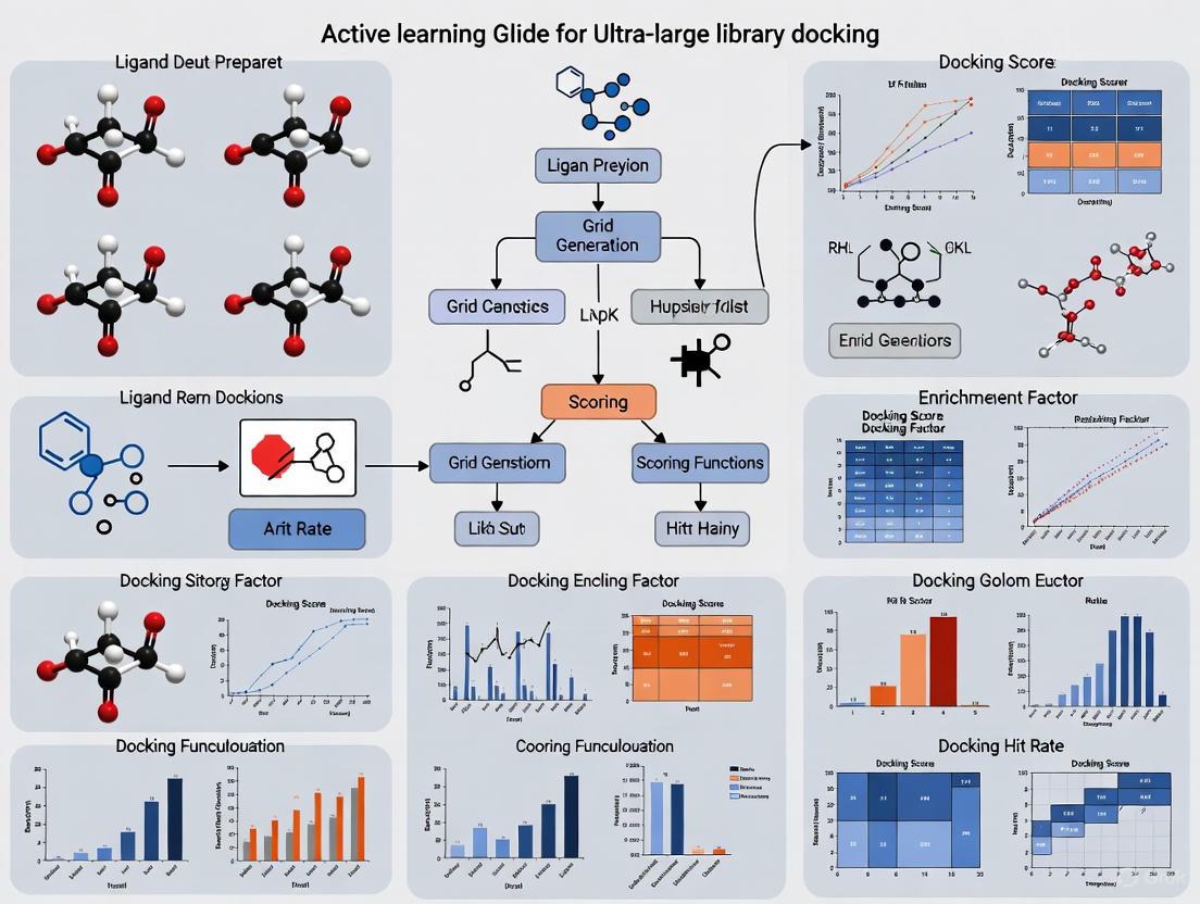
Implementing Active Learning Glide: A Step-by-Step Workflow for Screening Billions
Core Components of the Active Learning Glide Workflow
Active Learning Glide (AL-Glide) is a machine learning (ML)-augmented molecular docking workflow designed to efficiently identify high-scoring ligands from ultra-large chemical libraries containing billions of compounds. This methodology addresses the fundamental computational bottleneck of traditional brute-force docking, making the screening of vast chemical spaces feasible without a proportional increase in computational cost [4] [18]. The core principle involves an iterative, supervised learning cycle where a machine learning model is trained to become a accurate proxy for the Glide docking scoring function. This model then prioritizes which compounds to dock in subsequent cycles, effectively focusing computational resources on the most promising regions of chemical space [18].
The workflow is a cornerstone of modern virtual screening (VS), enabling researchers to achieve double-digit hit rates—a significant improvement over the 1-2% typical of traditional VS—while requiring only a fraction of the computational cost of an exhaustive screen [18]. By recovering approximately 70% of the top-scoring hits found through exhaustive docking at just 0.1% of the cost, AL-Glide has established itself as a critical tool for initial hit identification in structure-based drug design [4].
Workflow Diagram and Process
The following diagram illustrates the iterative, cyclical nature of the Active Learning Glide workflow.
Process Description
The AL-Glide workflow can be broken down into the following key stages, as shown in Figure 1:
- Library Initialization: The process begins with an ultra-large chemical library, often containing billions of purchasable compounds from sources like the Enamine REAL database [18] [10].
- Initial Batch Selection: An initial, manageable batch of compounds is selected at random from the full library for the first round of docking [18].
- Glide Docking & Scoring: The selected batch of compounds is docked against the protein target of interest using Glide, and each compound is assigned a docking score (e.g., GlideScore) [4] [18].
- Machine Learning Model Training: The compounds that were docked, along with their docking scores, are used to train a machine learning model. This model learns to approximate the relationship between a compound's features and its Glide docking score [18].
- ML-Based Library Prediction: The trained ML model is then used to rapidly predict the docking scores for the entire ultra-large library, a process that is orders of magnitude faster than actual docking [4] [18].
- Iterative Batch Prioritization: Compounds with the best-predicted scores from the ML model are selected to form the next batch for actual Glide docking. The workflow then returns to Step 3, creating a closed-loop cycle. With each iteration, the ML model is retrained on an increasingly large and informative set of docked compounds, improving its predictive accuracy and its ability to find high-scoring ligands [18].
- Final Output: After a predetermined number of cycles, the process terminates, yielding a final, curated list of top-scoring compounds that have been validated by full Glide docking. These compounds are then typically advanced to more rigorous scoring stages in a modern virtual screening pipeline [18].
Quantitative Performance Metrics
The performance of the Active Learning Glide workflow is characterized by high computational efficiency and robust recovery of top-tier hits, as summarized in the table below.
Table 1: Performance Metrics of Active Learning Glide
| Metric | Performance | Context / Comparison |
|---|---|---|
| Computational Cost Reduction | ~99.9% cost saving [4] | Compared to brute-force docking of an ultra-large library. |
| Top-Hit Recovery Rate | ~70% of top-scoring hits recovered [4] | Compared to the hits found from an exhaustive docking screen. |
| Virtual Screening Hit Rate | Double-digit hit rates (e.g., 14%, 44%) frequently achieved [18] [3] | Post-experimental validation; far exceeds traditional 1-2% rates. |
| Library Size Applicability | Billions of compounds [4] [10] | Successfully applied to screens of ~500 million compounds [10]. |
Detailed Experimental Protocol
This section provides a detailed, step-by-step protocol for setting up and running an Active Learning Glide screen, based on established methodologies [4] [18] [10].
System Preparation
Protein Target Preparation:
- Obtain a high-resolution 3D structure of the target protein (e.g., from PDB).
- Using Maestro's Protein Preparation Wizard, perform the following steps:
- Add missing hydrogen atoms.
- Assign appropriate protonation states at biological pH for residues, particularly His, Asp, Glu, and Lys.
- Optimize hydrogen bonding networks.
- Perform a restrained minimization to relieve steric clashes using the OPLS4 force field until the RMSD of heavy atoms converges to 0.3 Å.
Receptor Grid Generation:
- Within Glide, define the receptor grid for docking.
- Select the prepared protein structure.
- Define the centroid of the binding site using a co-crystallized ligand or known binding site residues.
- Set the inner box (bounding box) to enclose the ligand, typically defaulting to 10 Å from the centroid.
- Set the outer box (box size) to define the overall space sampled by the ligand, typically 20-30 Å depending on ligand size variability expected in the library.
Ligand Library Preparation:
- Source a commercial ultra-large library (e.g., Enamine REAL).
- Using LigPrep, standardize the compound structures:
- Generate possible tautomers and protonation states at a pH of 7.0 ± 2.0.
- Apply specified chirality.
- Perform energy minimization using the OPLS4 force field.
Active Learning Glide Execution
Initialization:
- In the Active Learning Applications interface, load the prepared receptor grid and ligand library.
- Configure the active learning parameters:
- Initial Batch Size: Typically 50,000-100,000 compounds, selected randomly.
- Selection Size per Cycle: The number of top ML-predicted compounds to dock in each subsequent cycle (e.g., 50,000-100,000).
- Number of Cycles: Typically 10-20 iterations, or until convergence is observed in the docking scores of the selected batches.
Iterative Active Learning Cycle:
- Cycle 1: The initial random batch is docked with Glide SP, and the docking scores are recorded.
- An ML model (e.g., a directed message passing neural network) is trained on the featurized compounds and their docking scores.
- The trained model predicts scores for the entire undocked library.
- The top N compounds with the best-predicted scores are selected for the next docking cycle.
- Cycles 2 to N: The newly selected batch is docked. The ML model is retrained on the accumulated set of all previously docked compounds and their scores. The process of prediction and selection repeats.
- Monitor the convergence by tracking the docking scores of the selected batches across cycles; the process can be stopped when the score distribution stabilizes.
Final Output:
- Upon completion of the specified cycles, the workflow outputs a list of the top-scoring compounds identified across all docking cycles. Full docking poses are available for these compounds.
Post-Processing and Hit Validation
Rescoring with Advanced Docking Methods:
- To improve pose prediction and initial enrichment, the top hits from AL-Glide (e.g., the best 10-100 million compounds) can be rescored using the more sophisticated Glide WS. Glide WS incorporates explicit water energetics from WaterMap, leading to a significant reduction in false positives and improved docking accuracy [15] [19] [18].
Absolute Binding Free Energy Perturbation (ABFEP+):
- A few thousand of the most promising compounds are subjected to rigorous free energy calculations using ABFEP+.
- This step provides a highly accurate prediction of binding affinity, closely correlating with experimental results, and is a linchpin for achieving high hit rates [18].
- An active learning approach can also be applied to ABFEP+ to scale the number of compounds evaluated with this expensive method [18].
Experimental Validation:
- The final, computationally validated hits are acquired or synthesized and tested in biochemical or cell-based assays to confirm biological activity, as demonstrated in the identification of a first-in-class WLS inhibitor [10].
The Scientist's Toolkit: Essential Research Reagents & Solutions
The successful implementation of the AL-Glide workflow relies on a suite of software tools and chemical resources. The following table details these essential components.
Table 2: Key Research Reagents and Solutions for AL-Glide
| Item Name | Function / Description | Role in the Workflow |
|---|---|---|
| Glide | Industry-leading ligand-receptor docking software. | Performs the core high-throughput docking and scoring of compound batches; provides the "ground truth" data for ML model training [15]. |
| Active Learning Applications (Schrödinger) | A powerful tool that integrates ML with docking. | Manages the iterative active learning cycle, including ML model training, prediction on the full library, and batch selection [4]. |
| Enamine REAL Library | An ultra-large, make-on-demand combinatorial chemical library. | Serves as the primary source of billions of synthetically accessible compounds for the virtual screen [10]. |
| FEP+ | A technology for performing free energy perturbation calculations. | Used for accurate rescoring of top hits via ABFEP+ to dramatically improve hit rates prior to experimental testing [4] [18]. |
| Glide WS | An advanced docking method incorporating explicit water dynamics. | Rescores top hits from AL-Glide to improve pose prediction and enrichment, helping to reduce false positives [15] [19] [18]. |
| Maestro (Schrödinger Suite) | A unified graphical user interface for computational life sciences. | Provides the integrated platform for protein prep, grid generation, workflow setup, and results analysis [4] [15]. |
The screening of ultra-large chemical libraries, often containing billions of commercially available compounds, has become a prominent strategy for in silico hit discovery in structure-based drug design [2] [3]. The fundamental premise is that larger libraries increase the probability of identifying high-affinity ligands, a concept often summarized as "the bigger, the better" [2]. However, the computational expense of exhaustively docking billions of compounds using physics-based methods like molecular docking is prohibitive for most research groups [2] [20]. For instance, screening 1.3 billion compounds utilizing 8,000 CPUs can require 28 days and cost over $200,000 [2].
Active learning (AL), a machine learning strategy, has emerged as a powerful solution to this challenge. This iterative framework intelligently selects the most informative compounds for expensive physics-based docking, training surrogate models to predict docking scores for the entire library at a fraction of the computational cost [4] [20]. By strategically sampling the chemical space, Active Learning Glide can recover approximately 70% of the top-scoring hits that would be found through exhaustive docking while requiring only 0.1% of the computational resources [4]. This Application Note details the protocols and practical considerations for implementing iterative model training within the context of ultra-large library docking research.
Key Performance Metrics and Comparative Analysis
The efficacy of active learning docking is validated through robust benchmarking studies. The following tables summarize key quantitative data and performance comparisons.
Table 1: Key Performance Metrics from Active Learning Docking Studies
| Metric | Reported Value | Context / Method | Source |
|---|---|---|---|
| Computational Cost Reduction | 99% (screening 1% of library) | HASTEN tool recall of top-scoring compounds [20] | [20] |
| Top-Hit Recall Rate | ~90% of top 1000 hits | HASTEN on a 1.56 billion compound library [20] | [20] |
| Hit Rate in Experimental Validation | 14% (KLHDC2), 44% (NaV1.7) | RosettaVS platform screening [3] | [3] |
| Screening Enrichment (EF1%) | 16.72 | RosettaGenFF-VS on CASF2016 benchmark [3] | [3] |
| Docking Time for Ultra-Large Library | < 7 days | OpenVS platform with 3000 CPUs and 1 GPU [3] | [3] |
Table 2: Comparison of Docking and Active Learning Strategies
| Method | Key Features | Advantages | Limitations |
|---|---|---|---|
| Brute-Force Docking | Exhaustive screening of entire library [20] | Maximum coverage; no bias [2] | Prohibitively high computational cost and time [2] [20] |
| Active Learning Glide | Iterative docking & ML model training; uses ensemble of RF and GCNN [4] [20] | Recovers ~70% of top hits for 0.1% cost [4] | Model performance depends on initial sampling and acquisition function [2] |
| HASTEN | Iterative docking using Chemprop neural network for score prediction [20] | 99% cost reduction; robust recall on giga-scale libraries [20] | Performance can be hampered by large numbers of failed docking compounds [20] |
| RosettaVS (OpenVS) | Open-source platform; combines VSX (fast) and VSH (high-precision) modes with active learning [3] | High accuracy; models receptor flexibility; open-source [3] | Requires substantial HPC infrastructure for ultra-large screens [3] |
Experimental Protocols for Active Learning Docking
This section provides detailed methodologies for setting up and executing an active learning virtual screening campaign.
Core Workflow of Active Learning for Molecular Docking
The following diagram illustrates the overarching iterative workflow of an active learning docking campaign.
Protocol 1: Standard Active Learning Docking Setup
This protocol is adapted from methodologies described for tools like HASTEN and Active Learning Glide [2] [20].
Step 1: Library Preparation
- Obtain the chemical library in SMILES format (e.g., Enamine REAL, ZINC).
- Standardization: Use tools like RDKit or Schrödinger LigPrep to standardize structures, generate canonical SMILES, and remove duplicates [20].
- Preparation for Docking: Prepare 3D structures with tools like LigPrep, generating relevant tautomers and stereoisomers at a physiological pH (e.g., 7.0 ± 1.5). Energy-minimize structures using a force field like OPLS_2005 [20].
Step 2: Receptor Preparation
- Obtain the 3D structure of the target protein from the PDB or via homology modeling.
- Processing: Prepare the protein structure using a tool like the Schrödinger Protein Preparation Wizard. This includes adding hydrogens, assigning bond orders, filling missing side chains, and optimizing hydrogen bonds.
- Grid Generation: Define the binding site and generate a docking grid centered on the region of interest.
Step 3: Initial Random Sampling and Docking
Step 4: Iterative Active Learning Cycle The core loop is detailed in the diagram below, which expands on the machine learning and acquisition steps.
- Step 5: Termination and Analysis
- Stopping Criterion: The cycle typically runs for a fixed number of iterations (e.g., 10-20) or until the top-ranked compounds stabilize and no longer change significantly.
- Output: The final output is a ranked list of top-scoring compounds from the entire library, generated from the model's predictions and the docked subsets.
Protocol 2: Handling Docking Failures and Constraints
A known challenge in ML-boosted docking is that some compounds fail to dock successfully, often due to conformational strain or the application of constraints (e.g., required hydrogen bonds) [20]. This protocol outlines mitigation strategies.
Step 1: Pre-Filtering
- Implement aggressive pre-filtering based on physicochemical properties (e.g., molecular weight, logP, rotatable bonds) to remove compounds unlikely to dock successfully or fit the binding pocket.
- Use functional group filters to remove reactive or undesirable species.
Step 2: Failed Compound Management
- During the docking steps, track and log compounds that fail to generate a valid pose or score.
- Strategy 1 (Exclusion): Assign a penalizingly poor score to failed compounds, ensuring the ML model learns to avoid similar structures in subsequent iterations.
- Strategy 2 (Separate Classifier): Train a separate binary classifier to predict the likelihood of a compound docking successfully. Use this classifier to filter the library before the acquisition step [20].
Step 3: Constraint-Aware Active Learning
- Be cautious when using stringent docking constraints, as they can increase failure rates and hamper ML learning [20].
- Consider applying constraints more leniently in the initial VS stage and applying them rigorously only during the final re-ranking of top hits.
Table 3: Key Research Reagent Solutions for Active Learning Docking
| Item / Resource | Function / Description | Example Tools / Sources |
|---|---|---|
| Ultra-Large Chemical Libraries | Source of purchasable or synthesizable compounds for virtual screening. | Enamine REAL, ZINC, ChemBridge [2] [20] |
| Molecular Docking Software | Physics-based program to predict protein-ligand binding poses and scores. | Glide, AutoDock Vina, RosettaVS, GOLD [4] [3] [21] |
| Active Learning Platform | Software that implements the iterative AL workflow for docking. | Schrödinger Active Learning Apps, HASTEN, OpenVS, MolPAL [4] [3] [20] |
| Machine Learning Framework | Library for building and training surrogate models for score prediction. | PyTorch, TensorFlow, Chemprop (for GNNs), Scikit-learn (for RF) [20] |
| Cheminformatics Toolkit | Library for handling molecular data, featurization, and pre-processing. | RDKit, Schrödinger LigPrep, OpenBabel [20] |
| High-Performance Computing (HPC) | Computational cluster with hundreds to thousands of CPUs and multiple GPUs. | Local HPC clusters, Cloud computing (AWS, GCP, Azure) [3] [20] |
Discussion and Technical Notes
Understanding the "Black Box": How 2D Models Predict 3D Affinity
A critical inquiry in active learning docking is how a surrogate model can accurately predict a docking score—a property rooted in 3D molecular interaction—using only 2D structural information. Analysis suggests that these models effectively memorize structural patterns that are prevalent in the high-scoring compounds sampled during the iterative process [2]. These patterns are not arbitrary; they correlate with specific three-dimensional shapes and interaction potentials (e.g., pharmacophores) that are complementary to the binding pocket. The model learns that certain molecular subgraphs or fingerprints are consistently associated with favorable docking outcomes for a specific target, enabling rapid and effective prioritization without explicit 3D calculation for every molecule [2].
Best Practices and Pitfalls
- Acquisition Function Choice: The Greedy and UCB strategies are most effective for finding top-scoring compounds, while Uncertainty sampling is better for model exploration and training [2].
- Initial Sampling: A sufficiently large and diverse initial random sample is crucial to prevent the model from getting trapped in a local optimum of chemical space.
- Validation: Always validate the final hit list by re-docking a sample of top-ranked compounds with a more precise, high-fidelity docking method (e.g., Glide SP or XP, RosettaVS VSH mode) [3].
- Generalizability: The surrogate model is highly target-specific. A model trained on one protein target cannot be directly applied to another.
In modern drug discovery, the ability to efficiently screen ultra-large chemical libraries containing billions of molecules presents both a substantial opportunity and a significant computational challenge. Active learning (AL) integrated with physics-based computational methods has emerged as a transformative solution, enabling researchers to navigate this vast chemical space with unprecedented efficiency. This application note details the implementation and synergy of two key active learning applications: Active Learning Glide (AL-Glide) for initial hit identification and Active Learning Free Energy Perturbation (AL-FEP+) for subsequent lead optimization. By framing these methodologies within a cohesive workflow, we provide researchers with a comprehensive protocol for accelerating the early drug discovery pipeline, from initial screening to optimized lead compounds.
Active Learning Glide (AL-Glide) for Hit Finding
Active Learning Glide (AL-Glide) addresses the fundamental challenge of screening ultra-large, make-on-demand chemical libraries, which can contain hundreds of millions to billions of readily available compounds [1] [10]. Traditional virtual screening methods, which rely on brute-force docking of entire libraries, become computationally prohibitive at this scale. AL-Glide combines the accuracy of the Glide docking program with cutting-edge machine learning to iteratively train a model that predicts docking scores, functioning as a rapid proxy for the more computationally expensive physics-based docking calculation [4] [18]. This approach allows for the identification of the most promising compounds for a fraction of the time and cost of an exhaustive screen.
Quantitative Performance
The performance of AL-Glide is demonstrated through its application across multiple drug discovery campaigns. The table below summarizes key quantitative benchmarks.
Table 1: Performance Metrics of AL-Glide in Ultra-Large Library Screening
| Metric | Performance | Context / Library Size | Source |
|---|---|---|---|
| Computational Efficiency | ~0.1% of the cost of exhaustive docking | Recovering ~70% of top-scoring hits | [4] |
| Hit Rate Improvement | Double-digit hit rates (e.g., >10%) achieved | Compared to 1-2% with traditional VS | [18] |
| Reported Application | Identification of a first-in-class WLS inhibitor | From ~500 million compounds | [10] |
| Comparative Docking Cost | Days | Versus months for brute-force docking | [4] |
Detailed Experimental Protocol
The following workflow delineates a standard protocol for a hit-finding campaign using AL-Glide.
Protocol Steps:
- Library and Protein Preparation: Begin with an ultra-large commercial library (e.g., Enamine REAL). Prepare the protein structure using the Schrödinger Protein Preparation Wizard, which involves adding hydrogen atoms, correcting ionization states, and performing a restrained energy minimization [22]. Generate a receptor grid file defining the binding site.
- Prefiltering: Filter the library based on desired physicochemical properties (e.g., molecular weight, lipophilicity) to remove undesirable compounds and focus on a relevant chemical space [18].
- AL-Glide Screening: Initiate the active learning cycle as depicted in the workflow diagram.
- An initial batch of compounds is selected from the library and docked with Glide.
- These docking scores are used to train a machine learning model.
- The trained model predicts the docking scores for the entire library.
- The model then selects the most informative compounds for the next round of docking and model retraining. This process iterates, with the model becoming increasingly accurate at identifying high-scoring compounds [18].
- Full Docking and Rescoring: Upon completion of the active learning cycles, the top several million compounds ranked by the ML model undergo a full Glide docking calculation. The resulting poses and scores are then refined using Glide WS (WaterScore), which explicitly models key water molecules in the binding site for more accurate scoring and pose prediction [18].
- Hit Selection and Validation: A final list of top-ranked compounds is selected for procurement and experimental validation in biochemical or cell-based assays.
Active Learning FEP+ (AL-FEP+) for Lead Optimization
Following hit identification, the lead optimization phase aims to explore diverse chemical analogs to improve potency and other drug-like properties. Active Learning FEP+ (AL-FEP+) is designed for this purpose, enabling the exploration of tens to hundreds of thousands of compounds by building machine learning models on free energy perturbation (FEP+) predicted affinities [4] [23]. FEP+ provides highly accurate, physics-based binding affinity predictions, but is computationally expensive. AL-FEP+ uses an active learning framework to minimize the number of required FEP+ calculations, using them to train an ML model that can accurately predict potency across a much larger virtual chemical space [4].
Quantitative Performance
AL-FEP+ has been rigorously tested in retrospective and prospective studies, demonstrating its impact on lead optimization.
Table 2: Performance and Application of AL-FEP+ in Lead Optimization
| Aspect | Finding | Context | Source |
|---|---|---|---|
| Chemical Space Exploration | Tens to hundreds of thousands of compounds | Per design objective | [4] |
| Model Performance | Well-performing models generated within several rounds | Especially when core is kept constant | [23] |
| Impact on Hit Rates | Contributes to achieving double-digit hit rates | In integrated modern VS workflow | [18] |
| Protocol Development | Active learning used to develop accurate FEP+ protocols | For challenging systems via FEP+ Protocol Builder | [4] |
Detailed Experimental Protocol
This protocol describes the use of AL-FEP+ to optimize a lead series by exploring a large, enumerated virtual library.
Protocol Steps:
- Define the Virtual Library: Start with a lead compound and generate a large virtual library (e.g., 100,000 - 1,000,000 compounds) through enumeration, exploring diverse R-groups, core changes, and bioisosteres [4].
- Initial FEP+ Calculations: Select a diverse subset of compounds from the virtual library (e.g., a few hundred) and run FEP+ calculations to obtain accurate binding affinity predictions.
- Active Learning Cycle:
- Train ML Model: Use the FEP+ results as training data to build a quantitative structure-activity relationship (QSAR) model. Schrödinger's AutoQSAR can be used for this, computing structural descriptors and employing multiple regression algorithms (e.g., PLS, KPLS) [22].
- Predict and Select: The trained model predicts the binding affinities for the entire enumerated library. An "explore-exploit" selection strategy is then applied. A portion of the next batch is selected from the top-predicted compounds (exploit), while another portion is chosen from chemically diverse or uncertain regions of the chemical space (explore) [23].
- Iterate with New FEP+: The newly selected compounds are processed with FEP+, and the results are added to the training set. The model is retrained, and the cycle repeats for several iterations (typically 3-5 rounds) [23] [22].
- Final Compound Selection: After the final active learning cycle, the ML model's predictions are used to identify the most promising compounds from the virtual library. These compounds are prioritized for synthesis and experimental testing based on their predicted high potency and favorable properties.
The Scientist's Toolkit: Essential Research Reagents and Solutions
The successful implementation of the workflows described above relies on a suite of specialized software tools and chemical resources.
Table 3: Key Research Reagents and Computational Solutions for Active Learning-Driven Discovery
| Tool / Resource | Type | Key Function in Workflow | Relevant Application |
|---|---|---|---|
| Enamine REAL Library | Chemical Library | Source of ultra-large, make-on-demand compounds for screening. | Hit Finding with AL-Glide [1] [10] |
| Glide | Software Module | Performs high-throughput molecular docking for pose prediction and scoring. | Foundational docking in AL-Glide [4] [18] |
| Active Learning Glide | Software Module | Machine learning layer that accelerates docking of billion-compound libraries. | Core of the hit-finding protocol [4] [18] |
| FEP+ | Software Module | Provides high-accuracy, physics-based binding free energy calculations. | Foundational for lead optimization [4] [18] |
| Active Learning FEP+ | Software Module | ML-guided selection for efficient FEP+ calculations on large virtual libraries. | Core of the lead optimization protocol [4] [23] |
| Glide WS | Software Module | Advanced docking rescoring that explicitly models water molecules for accuracy. | Rescoring post-docking [18] |
| AutoQSAR | Software Module | Automates the building and application of QSAR models using ML algorithms. | ML model training in AL-FEP+ [22] |
| Protein Preparation Wizard | Software Module | Readies protein structures for simulation by correcting structures and protonation states. | Essential pre-processing step [22] |
The Wnt signaling pathway is a fundamental biological system regulating cellular growth, development, and tissue homeostasis in animals [24]. Dysregulation of this pathway is implicated in numerous cancers, fibrotic diseases, and degenerative disorders, making it a significant therapeutic target [25] [24]. While previous drug discovery efforts have focused on upstream components like Porcupine (PORCN) or downstream effectors such as the β-catenin-TCF4 interaction, the integral membrane transporter Wntless (WLS) had remained an undrugged target despite its essential role in Wnt secretion [24] [26].
This case study details a successful structure-based drug discovery campaign that employed ultra-large scale virtual screening powered by Active Learning/Glide to identify the first-in-class WLS inhibitor, ETC-451, from a library of nearly 500 million compounds [25] [24] [10]. The research was framed within a broader thesis on applying advanced computational methods to access novel chemical space for challenging therapeutic targets.
Biological Context and Target Rationale
The Wnt Secretion Pathway and WLS Function
Wnt proteins are lipid-modified glycoproteins that require specialized machinery for their secretion and transport. The biosynthesis begins with the attachment of a palmitoleate moiety to Wnt by the endoplasmic reticulum-resident acyltransferase Porcupine (PORCN) [24]. This lipid modification is essential for the subsequent binding of Wnt to its dedicated transporter, Wntless (WLS), which facilitates secretion into the extracellular environment [24]. Once secreted, Wnt ligands initiate downstream signaling by binding to Frizzled receptors and co-receptors on target cells.
As the essential transporter for Wnt secretion, WLS represents a strategic bottleneck for modulating Wnt pathway activity. Genetic and preclinical data confirm that targeting WLS can effectively suppress signaling in Wnt-addicted cancers, validating its therapeutic potential [25] [24].
Target Druggability and Structural Insights
Recent advances in structural biology revealed that WLS contains a G-protein coupled receptor (GPCR) domain with a druggable binding pocket [25] [24] [10]. Cryo-EM structures of human WLS in complex with WNT8A and WNT3A show the bound palmitoleate moiety of Wnt inserted deeply into a hydrophobic cavity within the WLS transmembrane domain [24]. Structural homology searches and binding site detection analyses confirmed this pocket shares characteristics with canonical drug-binding sites in other GPCRs, suggesting susceptibility to small-molecule inhibition [24].
Diagram 1: WLS role in Wnt secretion pathway and cancer proliferation.
Computational Methodology
Virtual Screening Workflow Design
The virtual screening campaign followed a modern, multi-tiered workflow designed to efficiently navigate the ultra-large chemical space while maximizing the probability of identifying genuine hits. The protocol integrated machine learning-enhanced docking with rigorous physics-based rescoring to balance computational efficiency with predictive accuracy [18].
Key innovations included the use of Active Learning Glide (AL-Glide) to prioritize compounds for full docking calculations and the application of absolute binding free energy calculations (ABFEP+) for accurate affinity prediction across diverse chemotypes [18]. This approach addressed the fundamental limitations of traditional virtual screening, which had been constrained to smaller libraries (hundreds of thousands to few million compounds) and suffered from inaccuracies in scoring function-based ranking [18].
Structure Preparation and Binding Site Analysis
The virtual screening campaign initiated with the previously solved cryo-EM structure of the WNT8A-WLS complex (PDB). The Wnt ligand was removed from the complex, and the Sitemap tool (Schrödinger) was employed to identify and characterize potential druggable binding pockets on WLS [24]. This analysis revealed the GPCR-like transmembrane tunnel as the most promising binding site, designated Site 1, which featured partially polar residues at the top and predominantly hydrophobic residues lining the lower pocket [24].
Compound Library Preparation
The screening utilized Enamine's REAL 350/3 Lead-Like library, a make-on-demand collection containing approximately 500 million compounds with favorable physicochemical properties for drug discovery [24]. Library compounds adhered to stringent lead-like criteria: molecular weight between 270-350 Da, heavy atom count between 14-26, SlogP ≤ 3, and no more than 2 aryl rings [24]. These parameters ensured selected hits would provide optimal starting points for subsequent medicinal chemistry optimization.
Active Learning Glide Screening Protocol
The core screening methodology employed AL-Glide, which combines machine learning with molecular docking to efficiently prioritize compounds from ultra-large libraries [18] [24]. The protocol substantially reduced computational resources compared to brute-force docking of the entire library.
Diagram 2: Active learning Glide virtual screening workflow.
Step-by-Step AL-Glide Protocol:
- Initial Diversity Screening: A random diversity-based subset of 50,000 compounds was selected from the full library and docked against the WLS binding site using Glide SP mode [24].
- Machine Learning Model Training: The docking scores from the initial subset were used to train a DeepChem learning model, which learned to predict docking scores based on chemical features [24].
- Active Learning Cycles: The trained model predicted docking scores across the entire library, and additional rounds of docking and model retraining were performed to refine predictions (Figure S1A) [24]. This iterative process continued until the machine learning model became an accurate proxy for the docking method.
- Full Docking Calculation: The top 1 million compounds ranked by the active learning model were subjected to full Glide SP docking calculations to generate precise poses and scores [24].
- Rescoring with Explicit Water: The most promising compounds from Glide SP docking were rescored using Glide WS, which incorporates explicit water information in the binding site to improve pose prediction and enrichment over standard docking alone [18] [24].
Hit Selection and Compound Prioritization
From the top 10,000 ranked compounds, volume overlapping clustering was applied to classify compounds based on their spatial occupancy within the binding site [24]. This analysis identified 6 major clusters, with the largest cluster (containing 9,116 compounds) demonstrating the best mutual fitness between ligand shape and binding pocket architecture [24]. Additional filtering using Schrödinger's membrane permeability module and visual inspection for putative protein-ligand interactions yielded a final selection of 86 diverse compounds for synthesis and experimental testing [24].
Experimental Validation
Primary Screening and Hit Identification
Of the 86 compounds selected from virtual screening, 68 were successfully synthesized by Enamine and evaluated in a Wnt/β-catenin reporter assay using STF3A cells [24]. This cellular system consists of HEK293 cells with integrated WNT3A expression and a β-catenin responsive SuperTOPFlash (STF) luciferase reporter, providing a sensitive readout of Wnt pathway activity [24]. Following 48-hour treatment with test compounds, luciferase activity measurements identified ETC-451 as a promising hit that significantly reduced Wnt reporter activity [24].
Mechanism of Action Studies
Secondary assays confirmed ETC-451 functioned through the intended mechanism:
- WLS-WNT3A Interaction: ETC-451 effectively blocked the physical interaction between WLS and its cargo protein WNT3A, demonstrating direct target engagement [24].
- Target Gene Expression: Treatment with ETC-451 downregulated expression of endogenous Wnt target genes, confirming functional pathway inhibition at the transcriptional level [24].
- Cellular Proliferation: In Wnt-addicted pancreatic cancer cell lines, ETC-451 treatment significantly decreased cellular proliferation, validating the therapeutic potential of WLS inhibition [25] [24].
Key Research Reagents and Solutions
Table 1: Essential research reagents and solutions for WLS inhibitor discovery
| Reagent/Solution | Provider/Source | Function in Research Protocol |
|---|---|---|
| Enamine REAL 350/3 Library | Enamine | Nearly 500 million make-on-demand lead-like compounds for ultra-large virtual screening [24] |
| Schrödinger Suite | Schrödinger | Comprehensive software for molecular modeling, docking, and machine learning [18] |
| Active Learning Glide | Schrödinger | Machine learning-enhanced docking for efficient billion-compound screening [18] [24] |
| Glide WS | Schrödinger | Advanced docking with explicit water molecules for improved pose prediction [18] |
| STF3A Reporter Cell Line | Academic literature | HEK293 cells with WNT3A expression and β-catenin responsive luciferase reporter [24] |
| Wnt/β-catenin Reporter Assay | Laboratory established | Luciferase-based functional screen for Wnt pathway inhibition [24] |
Results and Discussion
Quantitative Screening Outcomes
The virtual screening campaign demonstrated exceptional efficiency and effectiveness, particularly when contrasted with traditional screening approaches:
Table 2: Virtual screening outcomes and efficiency metrics
| Screening Metric | Traditional VS | Modern VS with AL-Glide | WLS Campaign Results |
|---|---|---|---|
| Library Size | 100K - 5M compounds | Up to several billion compounds | 500 million compounds [24] |
| Computational Cost | Moderate | High but optimized via ML | 128-CPU cluster + NVIDIA V100 GPU [24] |
| Compounds Synthesized | ~100-500 | ~50-100 | 86 compounds ordered, 68 synthesized [24] |
| Typical Hit Rate | 1-2% [18] | Double-digit percentages [18] | One confirmed hit (ETC-451) from 68 tested [24] |
| Hit Quality | Variable, often weak | High potency, diverse chemotypes | First-in-class inhibitor with functional activity [25] |
Significance and Research Implications
The identification of ETC-451 represents a significant milestone in several respects:
- Target Validation: This work provides the first pharmacological evidence that WLS is druggable and that its inhibition represents a viable therapeutic strategy for Wnt-driven cancers [25] [24].
- Methodological Validation: The success demonstrates the power of modern virtual screening workflows to identify functional hits from ultra-large chemical spaces, achieving what was previously possible only through high-throughput experimental screening [18] [24].
- Chemical Starting Point: ETC-451 provides a valuable chemical scaffold for further structure- or ligand-based drug discovery campaigns targeting WLS [25] [24]. The researchers have made their top 10,000 ranked hits publicly available to accelerate collective efforts in targeting WLS [24].
This case study demonstrates a complete workflow from target identification through in vitro validation of a first-in-class WLS inhibitor using Active Learning/Glide for ultra-large library docking. The successful identification of ETC-451 from a 500-million compound library highlights how modern computational approaches can dramatically improve the efficiency and success of hit discovery campaigns for challenging targets. The integration of machine learning-guided docking with rigorous physics-based scoring and careful experimental validation provides a robust blueprint for future drug discovery efforts targeting difficult-to-drug proteins, particularly those with deep, cryptic, or complex binding sites.
Optimizing Performance and Troubleshooting Common Pitfalls in Active Learning Workflows
Ultra-large chemical libraries, containing billions of readily available compounds, present an unprecedented opportunity for drug discovery by dramatically expanding the explorable chemical space for hit identification [1] [5]. The primary challenge in screening these vast libraries lies in the immense computational cost of exhaustive physics-based docking methods, which becomes prohibitive at such scales [4] [1]. Active learning (AL) strategies address this challenge by iteratively training machine learning (ML) models on selectively chosen subsets of data, enabling efficient exploration of chemical space at a fraction of the computational cost of brute-force screening [4]. This Application Note details practical protocols for initial library selection and model training within the context of active learning for ultra-large library docking, specifically framing the content within the broader thesis of applying Active Learning Glide (Schrödinger) in research settings.
Quantitative Comparison of Screening Methodologies
The performance gains offered by active learning and other advanced screening algorithms are substantial when compared to traditional virtual high-throughput screening (vHTS). The following table summarizes key quantitative benchmarks from recent state-of-the-art methodologies.
Table 1: Performance benchmarks of ultra-large library screening methodologies.
| Methodology | Library Size | Computational Efficiency | Hit Rate Enrichment | Key Performance Metrics |
|---|---|---|---|---|
| Active Learning Glide (Schrödinger) | Billions of compounds | ~99.9% cost reduction; recovers ~70% of top hits vs. exhaustive docking [4] | High | Efficiently identifies top-scoring compounds from ultra-large libraries [4] |
| REvoLd (Evolutionary Algorithm) | 20+ billion compounds | 49,000 - 76,000 unique molecules docked per target [1] | 869 to 1622-fold vs. random selection [1] | Stable enrichment and discovery of new scaffolds in combinatorial spaces [1] |
| OpenVS/RosettaVS (AI-Accelerated) | Multi-billion compounds | Screening completed in <7 days using 3000 CPUs & 1 GPU [3] | 14% hit rate (KLHDC2); 44% hit rate (NaV1.7) [3] | State-of-the-art docking (EF1%=16.72) and screening power on CASF2016 [3] |
| Conventional Docking (Prospective) | 170 million compounds | Required 70 trillion complex samples (D4 receptor) [5] | Hit rates fell monotonically with docking score [5] | Successfully discovered new chemotypes and ultra-potent ligands (e.g., 180 pM agonist) [5] |
Protocols for Initial Library Selection and Model Training
Protocol 1: Active Learning Glide Setup and Execution
This protocol describes the application of Schrödinger's Active Learning Glide for screening ultra-large libraries to identify high-scoring compounds with minimal computational resources.
Key Research Reagents & Solutions:
- Ultra-large Chemical Library: A virtual compound library, such as the Enamine REAL space (over 20 billion molecules) or other make-on-demand libraries [1] [5].
- Schrödinger Software Suite: Licenses for Glide (for docking), Active Learning Applications, and Jaguar or other tools for physics-based property calculations [4].
- High-Performance Computing (HPC) Cluster: Infrastructure sufficient for parallelized docking and ML model training.
Procedure:
- Library Preparation: Curate the initial virtual library. While the entire ultra-large library (e.g., billions of compounds) is considered the search space, the AL process will only dock a small fraction.
- Initial Training Set Selection: Randomly select a small, diverse subset (e.g., 1,000-10,000 compounds) from the full library. Dock this initial set using Glide to generate the first set of training labels (docking scores or FEP+ predicted affinities) [4].
- ML Model Training: Train an initial machine learning model (e.g., a neural network) using the docked subset. The model learns to predict docking scores based on molecular features [4] [3].
- Iterative Active Learning Loop: a. Prediction: Use the trained ML model to predict scores for all undocked molecules in the full library. b. Selection: Identify and select the top-ranking molecules (e.g., those predicted to be most potent) according to the ML model. An additional diversity criterion can be applied to ensure broad exploration. c. Docking and Validation: Dock the selected molecules using Glide to obtain accurate physics-based scores. d. Model Retraining: Augment the training data with the newly docked molecules and their scores, then retrain the ML model.
- Termination and Analysis: Repeat steps 4a-4d for a predetermined number of iterations or until convergence (e.g., when the top-ranked compounds stabilize). The final model's predictions or the pool of docked high-scoring compounds are used to select candidates for synthesis and testing [4].
Protocol 2: REvoLd for Combinatorial Library Exploration
This protocol outlines the use of the REvoLd (RosettaEvolutionaryLigand) evolutionary algorithm for efficient screening of combinatorial make-on-demand libraries without full enumeration, incorporating full receptor and ligand flexibility.
Key Research Reagents & Solutions:
- Combinatorial Reaction Rules: Defined lists of substrates and chemical reactions that constitute the make-on-demand library (e.g., Enamine REAL space chemistry) [1].
- Rosetta Software Suite: Installation of Rosetta with the REvoLd application and RosettaLigand flexible docking protocol [1].
- Structural Model: A high-resolution protein structure of the drug target with a defined binding site.
Procedure:
- Parameter Optimization: Optimize the evolutionary protocol using a pre-docked subset of the library (e.g., 1 million molecules). Fine-tune parameters, including population size, selection pressure, and mutation/crossover rates [1].
- Initial Population Generation: Create a random starting population of 200 ligands by combining building blocks according to the library's reaction rules [1].
- Evaluation: Dock each ligand in the current population against the target using the flexible RosettaLigand protocol to obtain a fitness score (docking score) [1].
- Evolutionary Cycle: a. Selection: Select the top 50 highest-scoring ("fittest") individuals from the current generation to be parents [1]. b. Reproduction: * Crossover: Create new offspring ligands by recombining fragments from pairs of parent ligands. * Mutation: Introduce variations in offspring by: * Swapping single fragments with low-similarity alternatives. * Changing the reaction type and searching for compatible fragments [1]. c. New Generation Formation: Combine the newly generated offspring to form the next generation. The algorithm includes a second round of crossover and mutation on lower-scoring individuals to promote diversity [1].
- Iteration and Analysis: Repeat steps 3-4 for 30 generations. Conduct multiple independent runs (e.g., 20 runs) from different random seeds to explore diverse regions of the chemical space and mitigate local minima convergence. Analyze the unique, high-scoring molecules discovered across all runs for synthesis [1].
Workflow Visualization
Diagram 1: High-level screening strategy overview comparing Active Learning and Evolutionary Algorithm paths for ultra-large library screening.
The Scientist's Toolkit: Essential Research Reagents
Successful implementation of active learning for ultra-large library docking relies on several key software and data resources.
Table 2: Essential research reagents and computational tools for active learning-based docking.
| Tool/Resource | Type | Primary Function in Workflow |
|---|---|---|
| Schrödinger Active Learning Applications | Commercial Software Platform | Integrates ML with physics-based docking (Glide, FEP+) to efficiently screen ultra-large libraries [4] |
| Glide | Commercial Docking Software | Provides high-accuracy, physics-based docking scores used as training labels for the active learning model [4] |
| Enamine REAL Space | Make-on-Demand Chemical Library | A combinatorially generated, synthetically accessible virtual library of billions of compounds for screening [1] [5] |
| RosettaVS / REvoLd | Open-Source Software Suite | Offers state-of-the-art flexible docking and evolutionary algorithms for exploring combinatorial libraries without full enumeration [1] [3] |
| FEP+ | Free Energy Perturbation Tool | Used within active learning workflows (Active Learning FEP+) to accurately predict binding affinities for lead optimization [4] |
Addressing Sampling Bias and Ensuring Chemical Diversity in Results
In the realm of modern drug discovery, virtual screening of ultra-large chemical libraries has emerged as a powerful strategy for identifying novel therapeutic candidates. The advent of make-on-demand libraries, encompassing hundreds of millions to billions of readily synthesizable compounds, presents an unprecedented opportunity to explore vast chemical spaces [5]. However, this opportunity comes with significant computational and methodological challenges, particularly concerning sampling bias and chemical diversity.
Active learning, integrated with molecular docking platforms such as Glide, provides a framework to navigate these immense chemical spaces efficiently. Active learning is an iterative feedback process that selects the most informative data points for labeling based on model-generated hypotheses, continually refining the model with newly acquired data [27]. This approach is particularly valuable for overcoming the limitations of traditional virtual screening, especially when dealing with flawed labeled datasets and an ever-expanding exploration space [27].
Within this context, two interrelated issues demand careful attention. First, sampling bias can occur when the virtual screening process systematically overlooks certain regions of chemical space, potentially missing valuable chemotypes. Second, the goal of ensuring chemical diversity requires deliberate strategies to guarantee that identified hits represent structurally distinct scaffolds, thereby increasing the likelihood of discovering novel intellectual property and optimizing the exploration of chemical space. This application note details practical protocols to address these challenges within active learning-guided docking campaigns using Glide for ultra-large libraries.
Understanding the Challenges
Sampling bias in virtual screening can manifest in several ways, negatively impacting the outcomes of a drug discovery campaign.
- Algorithmic Bias: Docking algorithms and machine learning models may have inherent preferences for certain molecular features or scaffolds, potentially overlooking promising chemotypes that do not fit these preferences. Performance is highly dependent on the combined machine learning models used within the active learning framework [27].
- Representation Bias: If the initial training set or the library itself lacks diversity or is not representative of the target's bioactive chemical space, the screening results will be skewed. This is analogous to the undercoverage bias seen in general research, where parts of the population of interest are not accurately represented in the sample [28].
- Early Convergence: In iterative active learning processes, there is a risk of the model prematurely converging on a local optimum—a specific, narrow region of chemical space—thus failing to explore other potentially productive areas [1]. This can be exacerbated by overly greedy selection strategies that prioritize only the very highest-ranking molecules in each iteration.
The impact of these biases is profound. A biased screen can yield numerous hits from a single, narrow chemotype, failing to deliver the novel scaffolds often sought in early discovery. This lack of diversity can be detrimental to subsequent lead optimization efforts and limit the intellectual property potential of the results.
The Critical Role of Chemical Diversity
Chemical diversity is not merely a quantitative measure but a strategic asset in drug discovery. The value of exploring diverse chemotypes is twofold:
- Increased Probability of Success: Screening a diverse library increases the likelihood of identifying hits against a wider array of biological targets and binding sites. Natural products, celebrated for their profound impact on drug discovery, exemplify this principle; their inherent vast chemical diversity has evolved for optimal interactions with biological macromolecules [29] [30].
- Discovery of Novel Chemotypes: Ultra-large libraries, such as the Enamine REAL space, are prized for their scaffold diversity. For instance, a 170-million-compound library was found to represent over 10.7 million unique scaffolds [5]. Prospective screens against targets like AmpC β-lactamase and the D4 dopamine receptor successfully identified potent inhibitors with unprecedented chemotypes, such as a phenolate inhibitor of AmpC—a warhead previously unobserved for β-lactamases [5].
Table 1: Key Findings from Ultra-Large Library Docking Campaigns Demonstrating Diversity
| Target | Library Size | Hits Synthesized & Tested | Key Outcome Related to Diversity |
|---|---|---|---|
| AmpC β-lactamase | 99 million compounds | 44 molecules | Discovery of a novel phenolate inhibitor chemotype; multiple new scaffold families confirmed by crystallography [5] |
| D4 Dopamine Receptor | 138 million compounds | 549 molecules | 81 new chemotypes discovered; 30 were sub-micromolar, including a 180 pM agonist [5] |
Strategies and Protocols for Bias-Aware Diverse Screening
This section outlines a practical, multi-faceted approach to integrating bias mitigation and diversity enhancement into an active learning workflow with Glide.
Pre-Screening Phase: Library Curation and Preparation
Protocol 1: Strategic Library Design and Pre-Processing
- Leverage Make-on-Demand Libraries: Utilize commercially available, synthetically accessible ultra-large libraries (e.g., Enamine REAL, WuXi GalaXi) from partners like Schrödinger's Prepared Commercial Libraries [15]. These libraries are constructed from well-characterized reactions and building blocks, ensuring that virtual hits have a high probability of being synthesized for experimental validation [5] [1].
- Analyze Library Composition: Before screening, profile the library using chemical descriptors (e.g., molecular weight, logP, topological polar surface area) and scaffold analysis (e.g., Bemis-Murcko scaffolds) to understand its coverage of chemical space. This establishes a baseline for assessing the diversity of your results.
- Apply "Fair" Pre-Filters: When applying drug-likeness or property filters (e.g., lead-like ranges), ensure they are not inadvertently biased against certain valid chemotypes. Consider using relaxed criteria in initial stages to avoid excessive narrowing of the chemical space.
Integrating Diversity Selection into the Active Learning Loop
The core of mitigating bias lies in modifying the active learning cycle itself. The standard workflow involves model initialization, iterative querying, experimental labeling, and model update [27]. The key is to augment the query strategy.
Protocol 2: Diversity-Enhanced Active Learning for Glide Docking
Initialization: Start the active learning process with a structurally diverse set of molecules to seed the first batch. This can be achieved through:
- Stratified Sampling: Select molecules to cover a wide range of physicochemical properties, similar to stratified random sampling used to avoid bias in general research [28].
- Maximizing Scaffold Diversity: Select molecules representing many different Bemis-Murcko scaffolds.
Iterative Querying with Multi-Objective Selection: In each active learning cycle, do not select molecules based solely on the best docking score (e.g., Glide SP score). Instead, use a multi-criteria selection function.
- Cluster-Based Selection: Cluster the top-ranking molecules from Glide by molecular fingerprint (e.g., ECFP4) or scaffold. Select the top-ranked molecules from within each cluster to ensure representation across multiple chemotypes [5]. This prevents a single, high-scoring scaffold from dominating the selection.
- Explore-Exploit Trade-off: Dedicate a portion of each batch (e.g., 20-30%) to "exploration" – selecting molecules that are structurally dissimilar to all previously tested compounds, even if their scores are moderately high. This helps escape local minima and counteracts early convergence [1].
Model Update and Iteration: Update the active learning model with the new experimental data (activity labels for the tested compounds). The increasingly diverse training data will help the model make more generalizable predictions across chemical space in subsequent iterations.
The following workflow diagram illustrates this enhanced active learning protocol:
Active Learning with Diversity Enhancement
Post-Screening Analysis and Validation
Protocol 3: Assessing Output Diversity and De-risking Hits
- Diversity Metrics: After the screening campaign, quantify the diversity of the hit list. Calculate the pairwise Tanimoto similarity or the number of unique scaffolds represented. Compare this to the diversity of the initial library and the top-ranking molecules from a rigid, score-only ranking to demonstrate the value of your approach.
- Scaffold Hopping Analysis: Actively identify hits that are structurally distinct from known binders (as recorded in databases like ChEMBL). This was a key step in the ultra-large library docking campaign against AmpC and D4, where molecules resembling known inhibitors were explicitly excluded to prioritize novelty [5].
- Retrospective Analysis: Perform a "sensitivity analysis" by re-running parts of the active learning process with different initial seeds or selection parameters. If the final hit lists are substantially different, it may indicate residual sensitivity to initial conditions and potential sampling bias, guiding improvements for future campaigns.
Successful implementation of these protocols requires a suite of computational and experimental resources.
Table 2: Key Research Reagent Solutions for Bias-Aware Diverse Screening
| Item Name | Function / Application | Relevance to Bias & Diversity |
|---|---|---|
| Schrödinger Glide with Active Learning [15] | Core docking and virtual screening platform enhanced with machine learning to accelerate ultra-large library screening. | The integrated active learning framework provides the infrastructure for implementing the iterative, diversity-aware protocols described in this note. |
| Prepared Commercial Libraries (e.g., Enamine REAL) [15] | Fully prepared, purchasable compound databases encompassing vast chemical space (billions of compounds). | The foundation of diversity. These make-on-demand libraries provide access to millions of unique scaffolds, ensuring the chemical space being screened is itself diverse and synthetically accessible [5] [1]. |
| Clustering & Cheminformatics Tools (e.g., Canvas, RDKit) | Software for molecular fingerprinting, scaffold analysis, and clustering. | Essential for executing cluster-based selection and quantifying the diversity of both the input library and the output hit list. |
| Enzyme Assay Kits (e.g., for AmpC β-lactamase) | Biochemical assays for experimental validation of virtual hit activity and selectivity. | Critical for generating the high-quality labeled data required to update the active learning model and validate that diverse chemotypes are genuinely bioactive [5]. |
| Crystallography System | For determining protein-ligand co-crystal structures. | The gold standard for confirming that docked poses of novel chemotypes are accurate, as demonstrated with the novel AmpC inhibitors [5]. |
Concluding Remarks
Addressing sampling bias and ensuring chemical diversity are not secondary concerns but fundamental requirements for leveraging the full potential of ultra-large library docking. By adopting the protocols outlined here—strategic library curation, diversity-enhanced active learning cycles, and rigorous post-screening analysis—researchers can significantly improve the outcomes of their campaigns.
Integrating these strategies with powerful tools like Glide and its active learning extensions enables a more efficient and effective exploration of chemical space. This approach moves beyond simply finding the best-scoring molecules to discovering the best and most diverse set of molecules, thereby de-risking the drug discovery pipeline and maximizing the probability of identifying novel, potent, and optimizable therapeutic leads.
In the field of ultra-large library docking, the central challenge is the efficient navigation of chemical spaces containing billions of compounds. Active learning, particularly as implemented in Schrödinger's Active Learning Glide, has emerged as a powerful strategy to address this challenge by intelligently selecting subsets of compounds for detailed evaluation. This approach strategically balances the computational expediency of machine learning-based triage with the accuracy of physics-based docking methods like Glide FEP+. The core objective of parameter tuning within this framework is to identify operational sweet spots where computational resource expenditure is minimized without substantially compromising the quality and reliability of the predicted hits. This document provides detailed application notes and protocols for optimizing these critical parameters, framed within the broader context of active learning Glide research for drug discovery.
Core Quantitative Data on Performance Trade-offs
The optimization of an active learning workflow requires a clear understanding of the quantitative relationships between computational cost, model performance, and key adjustable parameters. The data summarized in the following tables provide benchmarks for expected performance and guidance for parameter selection.
Table 1: Benchmark Performance of Active Learning Glide vs. Exhaustive Docking
| Performance Metric | Exhaustive Docking | Active Learning Glide |
|---|---|---|
| Computational Cost | 100% (Baseline) | ~0.1% of exhaustive cost [4] |
| Top Hit Recovery Rate | ~100% (Baseline) | ~70% [4] |
| Virtual Screening Efficiency | N/A | >1000-fold reduction in cost [31] |
| Key Applicable Library Size | Millions to Billions | Multi-billion compounds [31] |
Table 2: Impact of Key Parameters on Model Performance and Cost
| Tuned Parameter | Impact on Prediction Accuracy | Impact on Computational Speed | Recommended Value/Range |
|---|---|---|---|
| Training Set Size | Sensitivity & precision improve with size, stabilizing at ~1M compounds [31]. | Larger sets increase initial training cost but optimize subsequent screening. | 1 million compounds [31] |
| Significance Level (ε) | Lower ε reduces the prediction error rate but may decrease sensitivity [31]. | Lower ε shrinks the virtual active set, drastically reducing docking cost. | Target-dependent (e.g., 0.08-0.12) [31] |
| Machine Learning Classifier | CatBoost with Morgan fingerprints showed optimal precision and sensitivity [31]. | CatBoost offered the least computational demands for training and prediction [31]. | CatBoost with Morgan2 Fingerprints [31] |
Detailed Experimental Protocols for Parameter Tuning
Protocol 1: Establishing the Training Set and Active Learning Model
This protocol details the initial setup of the active learning workflow, focusing on the selection and training of the machine learning model that will guide the virtual screening process.
Training Set Construction and Docking:
- Objective: To generate a labeled dataset for training a classifier to distinguish between high-scoring and low-scoring compounds.
- Procedure: a. Randomly select a representative subset of 1 million compounds from the full ultra-large library (e.g., Enamine REAL Space) [31]. b. Perform exhaustive molecular docking of this subset against the protein target of interest using Glide to obtain a docking score for each compound. c. Define an activity threshold based on the top-scoring 1% of the docked library to create binary labels (active/inactive) for the training data [31].
Classifier Training and Validation:
- Objective: To train a robust model that can predict docking scores based on molecular structure.
- Procedure: a. Feature Representation: Encode the chemical structures of the training set compounds using Morgan2 fingerprints (the RDKit implementation of ECFP4) [31]. b. Model Selection: Train a CatBoost classifier using the docking scores as labels. CatBoost is recommended for its optimal balance of speed and accuracy in this context [31]. c. Validation: Split the training data (e.g., 80/20) for proper training and calibration. Evaluate model performance on a held-out test set using metrics like sensitivity and precision [31].
Protocol 2: Optimizing the Significance Level (ε) for Screening
This protocol focuses on a critical optimization step: determining the significance level that controls the size of the library to be docked, thereby directly impacting the balance between speed and accuracy.
Conformal Prediction for Virtual Active Set Selection:
- Objective: To use the trained model to select a manageable subset of the full library for docking, with a controlled error rate.
- Procedure: a. Employ the Mondrian conformal prediction (CP) framework. The CP framework uses the trained model and a calibration set to assign normalized P-values to compounds in the full library [31]. b. Apply a significance level (ε). This parameter determines the maximum allowable error rate for predictions. Compounds with a P-value for the "active" class greater than (1-ε) are included in the "virtual active" set [31]. c. The virtual active set is then passed to the final, expensive docking stage.
Determining the Optimal Significance Level (ε_opt):
- Objective: To find the ε value that maximizes efficiency while maintaining acceptable sensitivity.
- Procedure: a. Analyze the relationship between ε and the resulting virtual active set size. A lower ε results in a smaller, more stringent set. b. The optimal significance level (εopt) is the value that maximizes the number of useful (single-label) predictions while maintaining high sensitivity (e.g., ~0.88) [31]. c. This value is target-dependent. For example, benchmarks have found εopt = 0.12 for the A2A adenosine receptor and ε_opt = 0.08 for the D2 dopamine receptor [31]. This step should be calibrated for each new target.
Protocol 3: Final Docking and Hit Identification
This is the final stage of the workflow, where the most promising compounds identified by the active learning process are rigorously evaluated.
High-Precision Docking:
- Objective: To obtain accurate binding poses and affinity rankings for the final candidate compounds.
- Procedure: a. Perform high-precision molecular docking (e.g., using Glide SP or VSH mode in RosettaVS) on the entire virtual active set identified in Protocol 2 [3]. b. This step involves more computationally expensive calculations, potentially including full receptor flexibility, to ensure the highest accuracy for the final ranking [3].
Hit Analysis and Prioritization:
- Objective: To select the most promising compounds for experimental validation.
- Procedure: a. Rank the docked compounds from the virtual active set based on their final docking scores. b. Apply post-docking filters (e.g., based on ligand strain energy, interaction patterns, or chemical diversity) to select a final list of hits for synthesis and biochemical testing.
Workflow Visualization
The following diagram illustrates the integrated workflow of the parameter-tuned active learning process for ultra-large library screening.
Active Learning Docking with Parameter Tuning
The Scientist's Toolkit: Research Reagent Solutions
Table 3: Essential Computational Tools for Active Learning-Guided Docking
| Tool/Solution | Function in Workflow | Key Features for Balancing Speed/Accuracy |
|---|---|---|
| Schrödinger Active Learning Applications [4] | Integrated platform for ML-accelerated docking screens. | Combines Glide/FEP+ with ML; claims ~70% hit recovery for 0.1% cost [4]. |
| CatBoost Classifier [31] | Machine learning model for predicting high-scoring compounds. | Optimal balance of speed and accuracy; handles categorical features (fingerprints) well [31]. |
| Conformal Prediction (CP) Framework [31] | Provides statistically valid confidence measures for ML predictions. | Allows control of error rate via significance level (ε); enables reliable set reduction [31]. |
| Morgan2 Fingerprints (ECFP4) [31] | Molecular descriptor representing compound structure. | High-performing feature representation for virtual screening QSAR models [31]. |
| RosettaVS (OpenVS Platform) [3] | Open-source, flexible docking platform with active learning. | Offers VSX (fast) and VSH (accurate) modes; supports receptor flexibility [3]. |
| Glide Docking [4] | High-accuracy molecular docking for final scoring. | Industry-standard for pose prediction and scoring; used for final ranking in the workflow [4]. |
The application of Active Learning Glide (AL Glide) for ultra-large library docking represents a transformative shift in early drug discovery. This methodology enables the screening of billion-molecule libraries, recovering approximately 70% of top-scoring hits at just 0.1% of the computational cost of exhaustive docking [4]. However, the full potential of this powerful hit identification tool is only realized when effectively integrated with downstream lead optimization workflows. This application note details the strategic coupling of AL Glide outputs with two critical technologies: FEP+ Protocol Builder for model optimization and the De Novo Design Workflow for chemical space exploration, creating a seamless, efficient, and predictive drug discovery pipeline.
Quantitative Workflow Advantages
Integrating these technologies creates significant efficiencies in computational cost and researcher time. The table below summarizes the key quantitative benefits.
Table 1: Performance Advantages of Integrated Active Learning Workflows
| Workflow Component | Key Performance Metric | Impact |
|---|---|---|
| Active Learning Glide | Virtual Screening Cost & Time | Reduces computational cost to 0.1% of exhaustive docking; screens billion-compound libraries in days [4]. |
| FEP+ Protocol Builder | Model Optimization Time | Generates optimized FEP+ protocols 4x faster than manual optimization, saving ~20 days per project [32]. |
| FEP+ Protocol Builder | Model Accuracy | Routinely outperforms human experts across diverse targets (e.g., improved RMSE for MCL1: 1.1 vs 1.5 kcal/mol) [32]. |
| De Novo Design Workflow | Exploration Scale | Enables exploration of tens to hundreds of thousands of compounds against multiple design objectives [4]. |
Integrated Workflow Protocol
The following diagram maps the complete integrated workflow, from initial library screening to optimized compound design.
Protocol 1: Hit Identification with Active Learning Glide
Objective: To efficiently identify potent hits from an ultra-large chemical library.
Methodology:
- Library Preparation: Compile a ultra-large library (e.g., 1-6.5 billion compounds) in a suitable format (e.g., SMILES).
- Receptor Preparation: Prepare the protein structure using the Protein Preparation Wizard in Maestro, ensuring correct bond orders, protonation states, and minimization with the OPLS4 force field [33].
- Active Learning Glide Setup:
- Input the prepared library and receptor.
- The active learning algorithm iteratively selects a small subset of compounds for docking with Glide.
- A machine learning model is trained on the docking scores and molecular features of the selected compounds.
- The model predicts the most promising compounds for the next round of docking, progressively refining its search.
- Output: A focused set of top-ranking hit compounds for further validation and optimization [4].
Protocol 2: FEP+ Model Optimization with FEP+ Protocol Builder
Objective: To establish a highly accurate FEP+ model for the target, especially when default settings are insufficient.
Methodology:
- Input Preparation:
- Protein-Ligand Complex: An experimentally resolved structure or a high-quality computational model.
- Training Ligands: A set of 10-20 congeneric ligands with known affinity data spanning 2-3 orders of magnitude.
- Automated Protocol Optimization:
- FEP+ Protocol Builder employs an active learning workflow to iteratively search the parameter space (e.g., ligand alignment, residue protonation states, simulation box size).
- It automatically runs FEP+ calculations on different parameter combinations, using the training set to evaluate accuracy (e.g., RMSE).
- Validation: The optimized protocol is validated against a held-out test set of ligands to ensure predictive performance and avoid overfitting.
- Output: A robust, target-specific FEP+ protocol ready for prospective application on novel compounds [32] [34].
Protocol 3: Lead Optimization via Active Learning FEP+ and De Novo Design
Objective: To explore vast chemical space and identify compounds that maintain or improve potency while meeting other drug-like criteria.
Methodology:
- Active Learning FEP+ for Potency:
- The hit compounds from AL Glide are used as a starting point.
- Active Learning FEP+ is used to screen tens to hundreds of thousands of virtual compounds, predicting their relative binding affinities with high accuracy and at a fraction of the cost of a full FEP+ study [4].
- De Novo Design Workflow Integration:
- Enumeration: Synthetically tractable molecules are generated using multiple enumeration strategies (e.g., Pathfinder for retrosynthesis-based analog generation) [33].
- Multi-parameter Filtering: The enumerated library is passed through an advanced filtering cascade (AutoDesigner) that scores compounds based on potency (using the Active Learning FEP+ model), selectivity, solubility, and other ADMET properties.
- Output Prioritization: The highest-ranking compounds that satisfy all design objectives are selected as optimized leads for synthesis and experimental testing [4].
The Scientist's Toolkit: Essential Research Reagents
Successful implementation of this integrated workflow relies on several key software components.
Table 2: Key Software Tools and Their Functions in the Integrated Workflow
| Tool Name | Primary Function | Key Application in Workflow |
|---|---|---|
| Maestro | Unified Graphical User Interface | Central platform for running all simulations, visualizing results, and managing data [33]. |
| Glide | Ligand-Receptor Docking | Provides high-throughput docking scores for the initial machine learning model in AL Glide [4]. |
| FEP+ | Free Energy Perturbation | Accurately predicts relative protein-ligand binding affinities for lead optimization [35]. |
| Active Learning Applications | Machine Learning Manager | Orchestrates the active learning loop for both docking (AL Glide) and free energy calculations (AL FEP+) [4]. |
| Protein Preparation Wizard | Protein Structure Preparation | Ensures the input protein structure is optimized for accurate simulations [33]. |
| OPLS4 Force Field | Molecular Mechanics Force Field | Provides the underlying physical model for energy calculations in Glide, FEP+, and MD simulations [33]. |
| Pathfinder | Retrosynthesis Analysis | Generates synthetically accessible analogs for exploration in the De Novo Design Workflow [33]. |
Case Study: Application to SARS-CoV-2 PLpro Inhibitors
A recent study demonstrates the power of integrating these workflows. Researchers aimed to design inhibitors of the SARS-CoV-2 Papain-like protease (PLpro) by optimizing the lead compound GRL-0617.
- Pathfinder-Driven Enumeration: Retrosynthesis analysis was used to generate analogs of GRL-0617 by replacing the naphthalene moiety with commercially available building blocks, yielding 89,529 design ideas [33].
- Active Learning QSAR: A total of 10 QSAR models were built using active learning, achieving strong statistical results (average R² > 0.70) to rapidly score the enumerated ideas [33].
- FEP+ Validation: The top 35 prioritized compounds were scored using FEP+ calculations. The workflow successfully identified the most active (e.g., compound 45, ΔG = -7.28 ± 0.96 kcal/mol) and inactive compounds, validating the design strategy before synthesis [33].
This case highlights the synergy between reaction-based enumeration, machine learning scoring, and rigorous physics-based free energy validation.
Benchmarking Success: Validation, Case Studies, and Comparative Analysis
In the field of structure-based drug discovery, virtual screening of ultra-large chemical libraries containing billions of "make-on-demand" compounds has become a powerful approach for hit identification [36]. However, the computational cost of exhaustively docking every compound in these libraries using traditional physics-based methods like Glide is often prohibitive, creating a significant bottleneck in the early stages of drug discovery [4]. Active learning, a machine learning paradigm that strategically selects the most informative compounds for labeling and model training, presents an innovative solution to this challenge [37]. This application note details how the integration of Active Learning Glide enables researchers to recover approximately 70% of the top-scoring hits that would be found through exhaustive docking while utilizing only 0.1% of the computational resources [4].
Performance Quantification
Comparative Efficiency Metrics
The quantitative performance of Active Learning Glide demonstrates substantial improvements in computational efficiency for ultra-large library screening. The table below summarizes the key comparative metrics:
Table 1: Performance Comparison of Docking Methods
| Performance Metric | Traditional Glide (Brute Force) | Active Learning Glide | Improvement Factor |
|---|---|---|---|
| Computational Cost | Reference (100%) | 0.1% | 1,000x reduction [4] |
| Hit Recovery Rate | Reference (100%) | ~70% | Preserves majority of valuable hits [4] |
| Hit Rate (STAT3-SH2 Domain) | Benchmark for comparison | 50.0% | Exceptional hit rate for challenging target [36] |
| Screening Efficiency | 1-2 million compounds [36] | Billions of compounds | Enables previously impossible screens [4] |
Economic Impact Assessment
The implementation of active learning translates to direct economic benefits in drug discovery campaigns. The significant reduction in computational resource requirements directly decreases associated costs and accelerates project timelines.
Table 2: Economic Impact of Active Learning Implementation
| Resource Factor | Traditional Docking | Active Learning Glide | Practical Implications |
|---|---|---|---|
| Compute Time | Days to weeks [4] | Significantly faster [4] | Enables rapid iterative screening cycles |
| Hardware Requirements | High-performance computing clusters | Feasible with optimized hardware [4] | Reduces infrastructure dependency |
| Methodology | "Brute-force" docking [36] | AI-based economic workflow [36] | Democratizes access to ultra-large libraries |
Active Learning Glide Protocol
The following diagram illustrates the iterative workflow of Active Learning Glide, highlighting the cyclical process of model training, inference, and strategic data selection:
Experimental Procedures
Protocol 1: Initial Dataset Preparation
Objective: Prepare a robust foundation for the active learning cycle by creating representative labeled and unlabeled datasets.
- Compound Library Acquisition: Obtain a synthetically accessible ultra-large library (e.g., Enamine REAL, Mcule-in-stock) [36].
- Library Pre-processing: Filter compounds using standard drug-like criteria (e.g., Lipinski's Rule of Five, Veber criteria) and remove pan-assay interference compounds (PAINS) [36].
- Initial Seed Selection: Randomly select a diverse subset of 5,000-10,000 compounds from the full library to form the initial training set (labeled pool, L) [38].
- Reference Docking: Dock the initial seed set using the standard Glide SP protocol to generate accurate binding scores for model training [39].
Protocol 2: Active Learning Iteration Cycle
Objective: Iteratively improve the machine learning model's predictive accuracy by strategically expanding the training set with the most informative compounds.
- Model Training: Train a machine learning model (e.g., deep neural network) on the current labeled set L to learn the relationship between chemical structures and docking scores [36].
- Model Inference & Selection: Use the trained model to predict docking scores for the entire unlabeled pool U. Apply the Least Disagree Metric (LDM) or related uncertainty-based sampling strategy to identify the most informative candidates for labeling [37].
- Strategic Batch Selection: Select a batch of 1,000-5,000 compounds from U with the highest uncertainty scores, ensuring chemical diversity through methods like k-means++ seeding [37].
- Targeted Docking & Validation: Perform high-accuracy Glide docking on the selected batch to obtain their true binding scores [4].
- Training Set Expansion: Add the newly docked compounds and their scores to the labeled set: L = L ∪ {(x, y)} [38].
Protocol 3: Performance Validation & Hit Identification
Objective: Validate the final model performance and identify high-confidence hit compounds for experimental testing.
- Stopping Criteria Assessment: Evaluate model convergence by tracking the change in hit list composition between iterations. Proceed to the next step when the top-ranked compounds stabilize (e.g., <5% change between cycles) [38].
- Final Model Application: Use the fully trained model to screen the entire ultra-large library and rank all compounds by their predicted docking scores.
- Hit Selection & Validation: Select the top 1-2% of predicted compounds for final validation using rigorous Glide docking [4].
- Experimental Triaging: Prioritize the final hit list based on docking scores, chemical novelty, and synthetic accessibility for purchase and experimental validation.
The Scientist's Toolkit
Research Reagent Solutions
Table 3: Essential Resources for Active Learning Glide Implementation
| Resource Name | Type | Function in Workflow | Key Features |
|---|---|---|---|
| Schrödinger Glide | Docking Software | Provides high-quality binding pose prediction and scoring for training data generation [4]. | Precise binding pose prediction; physics-based scoring functions [39]. |
| Enamine REAL Library | Chemical Database | Source of ultra-large, synthetically accessible compounds for screening [36]. | Billions of make-on-demand compounds; diverse chemical space [36]. |
| Active Learning Applications | ML-Accelerated Module | Implements the active learning cycle and machine learning model training [4]. | Integration with Glide; automated iteration management [4]. |
| Least Disagree Metric (LDM) | AL Selection Algorithm | Identifies the most informative unlabeled samples by measuring proximity to the model's decision boundary [37]. | Manages complex decision boundaries; computationally efficient estimator [37]. |
| OTAVAchemicals SH2 Library | Targeted Library | Benchmark for knowledge-based approaches; useful for validation [36]. | Curated compounds targeting specific protein domains [36]. |
Technical Discussion
Strategic Considerations
The efficiency of Active Learning Glide hinges on several key strategic considerations. The selection of the initial training set significantly impacts early learning phases; while random sampling is common, ensuring chemical diversity from the outset can accelerate model convergence [38] [40]. Furthermore, the choice of active learning strategy must balance exploration (diversity) and exploitation (uncertainty). Early benchmarks in materials science indicate that uncertainty-driven strategies and diversity-hybrid approaches like RD-GS outperform geometry-only heuristics, particularly in data-scarce initial phases [38].
The remarkable 50% hit rate achieved against the STAT3-SH2 domain, a challenging protein-protein interaction target, demonstrates the method's robustness. This performance is attributed to the active learning workflow effectively navigating complex binding landscapes where traditional methods struggle [36].
Validation and Generalizability
Robust validation is crucial for successful implementation. The performance of the underlying docking protocol used to generate training data is a critical limiting factor [36]. It is essential to retrospectively validate the docking setup using known active and decoy molecules before initiating a large-scale active learning campaign. While this application note focuses on Glide docking scores as the primary objective, the Active Learning FEP+ application demonstrates the framework's extensibility to other physics-based predictions, such as relative binding free energies, enabling the exploration of diverse chemical space in lead optimization [4].
The emergence of ultra-large, synthetically accessible chemical libraries, containing billions of molecules, has created unprecedented opportunities for hit discovery in drug development [18]. However, this vastness poses a significant challenge for traditional virtual screening (VS) methods, which are often computationally intractable at this scale and have historically yielded low hit rates of 1-2% [18]. The integration of active learning with molecular docking represents a paradigm shift, enabling efficient navigation of this expansive chemical space. This document details application notes and protocols for the experimental validation of hits identified through Active Learning Glide (AL-Glide), providing a framework for progressing from in-silico predictions to synthesized, potent inhibitors within the context of a modern VS workflow [4] [18].
The Modern Virtual Screening Workflow
The modern VS workflow leverages machine learning to amplify physics-based calculations, dramatically improving efficiency and hit rates [18]. This multi-tiered process is designed to rigorously filter billions of compounds down to a select few promising candidates for experimental testing.
The following diagram illustrates the key stages of this workflow, from initial screening to experimental confirmation:
Core Computational Protocols
Protocol 1: Ultra-large Library Screening with Active Learning Glide
- Objective: To efficiently identify the most promising compounds from a library of several billion molecules.
- Method:
- Library Preparation: Obtain commercially available ultra-large libraries (e.g., Enamine REAL). Pre-filter based on physicochemical properties (e.g., molecular weight, logP) to remove undesired compounds [18].
- Active Learning Cycle: Implement an iterative machine learning process [4] [18]:
- A small, diverse batch of compounds is selected from the full library and docked using GLIDE.
- These docking results are used to train a machine learning (ML) model.
- The trained ML model predicts the docking scores for the entire library.
- The next batch of compounds is selected based on the ML model's predictions, focusing on regions of chemical space with high predicted scores.
- The process repeats, with the ML model becoming increasingly accurate at identifying high-scoring compounds.
- Outcome: A ranked list of millions of top-scoring compounds, achieved at a fraction of the computational cost of exhaustive docking [4].
Protocol 2: Rescoring with Glide WS and Absolute Binding FEP+
- Objective: To improve the accuracy of binding affinity predictions and reduce false positives.
- Method:
- Glide WS Rescoring: Subject the best-scoring compounds (typically hundreds of thousands to millions) from the previous step to rescoring with Glide WS. This advanced docking program incorporates explicit water molecules in the binding site, leading to more accurate pose prediction and enrichment [18].
- Absolute Binding FEP+ (ABFEP+): Perform rigorous free energy calculations on the top-ranked compounds (thousands) from Glide WS [18].
- ABFEP+ calculates the absolute binding free energy between the ligand and protein, without requiring a known reference compound.
- This step provides a near-quantitative prediction of binding affinity, with accuracy matching experimental methods.
- Outcome: A final, highly curated list of tens to hundreds of compounds with predicted high binding affinity and diverse chemotypes, ready for experimental validation.
Quantitative Workflow Performance
The following table summarizes the typical data volume and key outcomes for each stage of the modern VS workflow, demonstrating its efficiency.
Table 1: Performance Metrics of a Modern Virtual Screening Workflow
| Workflow Stage | Typical Library Size | Key Software/Tool | Primary Outcome |
|---|---|---|---|
| Initial Screening | Several Billion compounds | Active Learning Glide [4] [18] | ~70% recovery of top hits at ~0.1% computational cost [4] |
| Standard Docking | 10 - 100 Million compounds | GLIDE [41] [18] | Ranked list based on docking scores |
| Advanced Rescoring | Hundreds of Thousands | Glide WS [18] | Improved poses and enrichment |
| Potency Prediction | Thousands | Absolute Binding FEP+ (ABFEP+) [18] | Accurate binding affinity predictions |
| Experimental Output | Tens of compounds | Cell-based & biochemical assays [41] [18] | Double-digit hit rates (e.g., >10%) [18] |
Experimental Validation Protocols
Rigorous experimental validation is critical to confirm the computational predictions and identify true hits.
Primary Biochemical Assays
Protocol 3: Determination of Half-Maximal Inhibitory Concentration (IC50)
- Objective: To quantitatively measure the potency of synthesized hits in a cell-free system [41].
- Method:
- Reaction Setup: Prepare a buffer containing the purified target protein (e.g., kinase, protease) and its substrate. Include necessary co-factors.
- Dose-Response: Serially dilute the synthesized hit compounds across a range of concentrations (e.g., from 10 µM to 1 nM). Add each concentration to the reaction mixture.
- Activity Measurement: Initiate the enzymatic reaction and measure the initial velocity of product formation. This can be done via fluorescence, luminescence, or absorbance, depending on the assay.
- Data Analysis: Plot the percentage of enzyme activity remaining against the logarithm of compound concentration. Fit the data to a sigmoidal dose-response curve to determine the IC50 value [41].
- Validation Criterion: A compound is considered a confirmed hit if it demonstrates a statistically significant IC50, typically below 10 µM, with many high-quality hits showing sub-micromolar potency [41].
Cellular Functional Assays
Protocol 4: Validation of Cellular Efficacy and Cytotoxicity
- Objective: To confirm that the hit compound can penetrate cells and modulate the intended target in a biologically relevant environment [41].
- Method:
- Cell Line: Use a cell line that expresses the target protein and is relevant to the disease pathology.
- Treatment: Treat cells with the hit compound across a range of concentrations for a defined period.
- Efficacy Readout: Measure a downstream phenotypic or biomarker outcome. For example:
- For a kinase target, measure phosphorylation levels of a key substrate via Western blot.
- For an oncology target, assess cell proliferation or viability using assays like MTT or CellTiter-Glo.
- Cytotoxicity: Perform a parallel assay (e.g., LDH release) in primary or non-target cells to assess compound selectivity and general cytotoxicity.
- Validation Criterion: A potent hit will show a dose-dependent effect on the cellular pathway without significant cytotoxicity at the effective concentrations.
Case Study: Application to Diverse Targets
The integrated computational and experimental workflow has been successfully applied across multiple projects. A benchmark analysis indicated that active learning protocols, such as AL-Glide, effectively recover a high percentage of top-scoring molecules from ultra-large libraries while maintaining chemical diversity [42].
Table 2: Experimental Validation Outcomes Across Multiple Targets
| Target Class | Target Name | Docking Software | Number of Hits/Tested | Potency of Best Hit (IC50/EC50/Ki) | Cellular Assay | Animal Test |
|---|---|---|---|---|---|---|
| Kinase [41] | HK-2 | GLIDE | Data from source | Data from source | Reported [41] | Not Specified |
| Antimicrobial Target [41] | Mg2+ Transporter | Not Specified | Data from source | Data from source | Not Specified | Not Specified |
| Diverse Targets (Schrödinger) [18] | Multiple | Active Learning Glide | N/A | Low nM to µM range | Conducted | Not Specified |
The Scientist's Toolkit: Essential Research Reagents and Solutions
Successful execution of the validation pipeline requires a suite of specialized computational and experimental tools.
Table 3: Key Research Reagent Solutions for Hit Validation
| Item Name | Function / Application | Specific Example(s) |
|---|---|---|
| Ultra-large Chemical Libraries | Source of compounds for virtual screening; provides extensive coverage of chemical space. | Enamine REAL library [18] |
| Active Learning Glide | Machine-learning accelerated molecular docking for screening billions of compounds [4] [18]. | Schrödinger Active Learning Applications [4] |
| Absolute Binding FEP+ (ABFEP+) | High-accuracy computational protocol for predicting protein-ligand binding free energies [18]. | Schrödinger FEP+ [18] |
| Purified Target Protein | Essential reagent for in vitro biochemical assays to determine binding affinity and inhibitory potency. | Rho-associated protein kinase 2 (ROCK2) [43] |
| Cell-Based Reporter Assays | Systems for evaluating cellular permeability, functional activity, and cytotoxicity of hits. | Cell proliferation, phosphorylation, mitophagy assays [43] |
The expansion of ultra-large, make-on-demand chemical libraries, containing billions of synthesizable compounds, presents a golden opportunity for drug discovery [1]. However, this opportunity is coupled with the significant challenge of computationally screening these vast spaces in a feasible and efficient manner. Traditional virtual high-throughput screening (vHTS) with exhaustive molecular docking is often prohibitively expensive. In response, advanced computational strategies that prioritize smart sampling over brute-force calculation have been developed. Among these, active learning (AL) protocols have emerged as a powerful solution for accelerating structure-based virtual screening. This application note provides a comparative performance analysis of Schrödinger's Active Learning Glide against other state-of-the-art docking strategies, including Vina-MolPAL, SILCS-MolPAL, and the evolutionary algorithm REvoLd, focusing on their application in ultra-large library screening.
A direct benchmark of active learning protocols across different docking engines reveals significant differences in their performance and optimal use cases. The table below summarizes key quantitative findings from recent studies.
Table 1: Comparative Performance of Ultra-Large Library Screening Strategies
| Method | Key Performance Metric | Computational Efficiency | Key Advantage |
|---|---|---|---|
| Active Learning Glide | Recovers ~70% of top hits from exhaustive docking [4] | 0.1% cost of exhaustive docking [4] | Tight integration with physics-based Glide docking and FEP+ [4] |
| Vina-MolPAL | Achieved the highest top-1% recovery in a benchmark study [42] | Not specified | High accuracy in identifying top-tier binders [42] |
| SILCS-MolPAL | Comparable accuracy and recovery to top performers at larger batch sizes [42] | Not specified | Realistic description of membrane environments [42] |
| REvoLd (Evolutionary) | Hit rate improvements by factors of 869 to 1622 over random selection [1] | 49,000-76,000 unique molecules docked per target [1] | Full ligand and receptor flexibility via RosettaLigand [1] |
| Generative AI (VAE-AL) | 8 out of 9 synthesized molecules showed in vitro activity for CDK2 [44] | Not specified | De novo generation of novel, synthesizable scaffolds [44] |
Detailed Experimental Protocols
To ensure reproducibility and provide a clear guide for implementation, this section outlines the detailed methodologies for the key strategies discussed.
Protocol for Active Learning Glide Screening
The following protocol is adapted from studies screening natural compound libraries and ultra-large commercial libraries [4] [22].
System Preparation:
- Protein Preparation: Use the Schrödinger Protein Preparation Wizard to refine the protein structure. Steps include adding missing hydrogen atoms, correcting metal ionization states, assigning bond orders, optimizing the hydrogen bond network via protonation state sampling (e.g., for histidine residues), and performing a restrained minimization [22].
- Receptor Grid Generation: Define the binding site using the prepared protein structure. A grid is generated around the relevant binding cavity to confine the docking search space [22].
- Ligand Library Preparation: Prepare the ligand library (e.g., the TargetMol Natural Compound Library or an ultra-large make-on-demand library) by generating 3D structures and assigning protonation states at a physiological pH [22].
Initial Docking and Model Training:
- Initial Docking Round: Perform a standard Glide SP docking run on a subset of the library (e.g., 1-5% of compounds) to generate initial training data [4].
- Machine Learning Model Training: Train a machine learning model, such as a deep learning QSAR model (e.g., DeepAutoQSAR), using the docking scores as the target property. The model learns to predict docking scores based on the ligands' structural features [22].
Iterative Active Learning Cycles:
- Prediction and Selection: Use the trained ML model to predict the docking scores for all undocked molecules in the full library.
- Informed Batch Selection: Select the next batch of ligands for docking based on the model's predictions, typically focusing on compounds predicted to have the best scores, while potentially incorporating diversity or uncertainty sampling to improve the model.
- Model Retraining: The newly docked ligands and their scores are added to the training set, and the ML model is retrained. Steps 3a and 3b are repeated for a predetermined number of iterative training rounds (e.g., 3 rounds) [22].
Final Validation:
- After the final active learning cycle, the top-ranked ligands predicted by the final model are docked using Glide SP to validate their poses and scores [22].
Protocol for REvoLd Screening
The REvoLd protocol employs an evolutionary algorithm to explore combinatorial chemical space without full enumeration [1].
Initialization:
- Define Chemical Space: Specify the combinatorial library by its lists of substrates and known chemical reactions (e.g., the Enamine REAL space).
- Generate Starting Population: Create an initial random population of 200 unique molecules from the defined chemical space [1].
Evolutionary Optimization Cycle (Repeat for ~30 Generations):
- Docking and Fitness Evaluation: Dock all individuals in the current population using the flexible RosettaLigand protocol to obtain a docking score as the fitness function [1].
- Selection: Select the top 50 individuals (the "fittest") based on their docking scores to advance to the next generation [1].
- Reproduction (Crossover and Mutation): Create a new generation from the selected individuals by applying:
- Crossover: Recombine fragments of high-scoring molecules to create novel offspring.
- Mutation: Introduce random changes, such as switching single fragments to low-similarity alternatives or changing the reaction scheme, to foster diversity and exploration [1].
- Duplicate Removal: Ensure all newly generated molecules are unique to avoid redundant calculations.
Output: After the final generation, the algorithm outputs all unique molecules docked during the run, which includes many promising, high-scoring hits identified through the evolutionary process [1].
Protocol for Generative AI with Active Learning
This protocol integrates a generative model within nested active learning cycles for de novo molecule design [44].
Initial Model Training:
- A Variational Autoencoder (VAE) is first pre-trained on a general dataset of drug-like molecules to learn a robust latent representation.
- The VAE is then fine-tuned on a target-specific training set to bias generation towards relevant chemotypes [44].
Inner Active Learning Cycle (Guided by Chemoinformatics):
- Generation: The VAE decoder is sampled to generate new molecules.
- Cheminformatics Filtering: Generated molecules are evaluated for drug-likeness, synthetic accessibility (SA), and dissimilarity from the training set.
- Model Refinement: Molecules passing these filters are added to a temporal set, which is used to fine-tune the VAE. This inner cycle runs for multiple iterations to accumulate a pool of high-quality, synthesizable candidates [44].
Outer Active Learning Cycle (Guided by Physics-Based Scoring):
- After several inner cycles, an outer cycle is triggered.
- Docking Evaluation: The accumulated molecules in the temporal set are evaluated using molecular docking.
- Selection and Retraining: Molecules meeting a docking score threshold are transferred to a permanent set. The VAE is then fine-tuned on this permanent set, directly coupling the generative process to the physics-based affinity prediction [44].
Candidate Refinement and Selection:
- The most promising generated molecules from the permanent set undergo more intensive molecular modeling, such as Monte Carlo simulations (e.g., with PEL) or absolute binding free energy (ABFE) calculations, for final prioritization [44].
Workflow Visualizations
The following diagrams illustrate the logical flow of the key computational strategies.
Active Learning Glide Workflow
REvoLd Evolutionary Algorithm Workflow
Generative AI with Nested Active Learning
The Scientist's Toolkit: Essential Research Reagents & Solutions
The following table details key software and computational resources essential for implementing the discussed strategies.
Table 2: Key Research Reagent Solutions for Advanced Docking
| Item Name | Function / Application | Relevant Strategy |
|---|---|---|
| Schrödinger Suite (Glide, Protein Prep Wizard, DeepAutoQSAR) | Integrated platform for protein prep, molecular docking, and machine learning-based active learning. | Active Learning Glide [4] [22] |
| AutoDock Vina | A widely used open-source docking engine for predicting ligand binding modes and affinities. | Vina-MolPAL [42] |
| SILCS Suite | Docking and MC simulation platform that incorporates explicit cell membrane and solvent effects. | SILCS-MolPAL [42] |
| Rosetta Software Suite (REvoLd & RosettaLigand) | A comprehensive macromolecular modeling suite enabling flexible protein-ligand docking and evolutionary library screening. | REvoLd [1] |
| Enamine REAL Database | An ultra-large "make-on-demand" virtual library of billions of readily synthesizable compounds. | REvoLd, Active Learning Glide [1] |
| GROMACS | A high-performance molecular dynamics package used for system equilibration, simulation, and conformational analysis. | System refinement & validation [22] |
Molecular docking remains a cornerstone of structure-based drug design, enabling researchers to predict how small molecules interact with protein targets. The field is currently characterized by a dynamic interplay between established traditional methods and innovative deep learning (DL) approaches. Traditional tools like Glide are renowned for their robustness and high physical plausibility, whereas emerging DL algorithms offer transformative potential in speed and pose accuracy [39] [45]. This application note provides a systematic, multi-dimensional comparison of Glide's performance against contemporary DL and other classical docking programs. Framed within the context of ultra-large library docking research, we focus on critical metrics such as pose prediction accuracy, physical validity, and virtual screening (VS) efficacy to guide tool selection for modern drug discovery campaigns.
Performance Benchmarking: Glide vs. Deep Learning & Traditional Methods
Quantitative Comparison of Docking Accuracy and Physical Validity
A comprehensive multi-dimensional evaluation reveals the distinct strengths and weaknesses of various docking paradigms. The benchmarking, conducted across diverse datasets like the Astex diverse set, PoseBusters set, and DockGen, classifies methods into four performance tiers based on their combined success rate (RMSD ≤ 2 Å and PoseBusters-valid) [39].
Table 1: Performance Benchmarking Across Docking Paradigms (PoseBusters Benchmark Set)
| Method | Paradigm | RMSD ≤ 2 Å (%) | PB-Valid Rate (%) | Combined Success Rate (%) |
|---|---|---|---|---|
| Glide SP | Traditional (Physics-Based) | 70.09 | 97.20 | 69.16 |
| AutoDock Vina | Traditional (Physics-Based) | 51.40 | 95.79 | 50.47 |
| Interformer | Hybrid (AI Scoring) | 67.76 | 89.25 | 59.35 |
| SurfDock | Generative Diffusion (DL) | 77.34 | 45.79 | 39.25 |
| DiffBindFR (MDN) | Generative Diffusion (DL) | 50.93 | 47.20 | 33.88 |
| KarmaDock | Regression-Based (DL) | 17.76 | 31.78 | 8.88 |
| DynamicBind | Generative Diffusion (DL) | 14.02 | 26.17 | 5.61 |
The data shows that traditional methods, particularly Glide SP, consistently excel in producing physically plausible structures, maintaining PB-valid rates above 97% across all tested datasets [39]. This indicates a strong adherence to chemical and geometric constraints, which is critical for reliable drug design. Furthermore, Glide achieves the highest combined success rate, demonstrating a superior ability to generate poses that are both accurate and physically valid.
In contrast, generative diffusion models like SurfDock show exceptional pose accuracy, even outperforming other methods on novel protein binding pockets in the DockGen dataset [39]. However, this often comes at the cost of physical validity, as their PB-valid rates are frequently below 50%. This suggests that while they can identify correct binding regions, they often fail to model the precise physicochemical interactions correctly. Regression-based DL models consistently underperform in both pose accuracy and physical validity [39].
Virtual Screening Enrichment and Broader Benchmarking
Beyond pose prediction, a critical function of docking tools is to enrich true active compounds during virtual screening. Historical and recent studies consistently place Glide as a top performer in this area.
Table 2: Virtual Screening Enrichment Performance
| Method | Performance Highlights | Context |
|---|---|---|
| Glide XP | "consistently yield enrichments superior" to GOLD and DOCK | Diverse set of pharmaceutically interesting targets [8] |
| Glide | One of the two best protocols (with TankBind_local) for docking at Protein-Protein Interaction (PPI) interfaces | Benchmarking against AF2 models and native structures [46] |
| Active Learning Glide | Recovers ~70% of top-scoring hits from exhaustive docking at 0.1% of the cost | Ultra-large library screening (>500M compounds) [4] |
A landmark comparative study concluded that the "Glide XP methodology is shown to consistently yield enrichments superior to the two alternative methods (GOLD and DOCK)" [8]. This robustness extends to challenging targets like protein-protein interfaces (PPIs), where a 2025 benchmark identified Glide as one of the two best-performing protocols for local docking [46].
Experimental Protocols for Benchmarking Docking Accuracy
To ensure reproducibility and provide a framework for internal validation, we outline the core experimental protocols used in the cited benchmarks.
Protocol 1: Multi-Dimensional Docking Evaluation
This protocol is adapted from the comprehensive evaluation by Li et al. (2025) [39].
- 1. Dataset Curation:
- Astex Diverse Set: Used for evaluating performance on known, high-quality complexes.
- PoseBusters Benchmark Set: Provides a challenge set of unseen complexes to test generalization.
- DockGen Dataset: Curated to include novel protein binding pockets not represented in common training data, testing generalization to truly novel targets.
- 2. Pose Prediction and Accuracy Measurement:
- Run each docking program to generate top-ranked poses for all complexes in the benchmark sets.
- Calculate the Root-Mean-Square Deviation (RMSD) between the predicted ligand pose and the experimentally determined crystal structure pose.
- Report the success rate as the fraction of complexes where the RMSD is ≤ 2.0 Å.
- 3. Physical Validity Assessment:
- Process all predicted poses through the PoseBusters toolkit.
- The tool checks for violations of chemical and geometric constraints, including bond lengths, bond angles, stereochemistry, and protein-ligand steric clashes.
- A pose is considered "PB-valid" only if it passes all these checks.
- 4. Combined Metric Calculation:
- The combined success rate is the fraction of complexes for which a method produces a pose that is simultaneously accurate (RMSD ≤ 2 Å) and physically valid (PB-valid).
Protocol 2: Virtual Screening Enrichment Evaluation
This protocol is standard for assessing a method's ability to identify active compounds from a large database of decoys [8].
- 1. Dataset Preparation:
- For a target protein, compile a set of known active compounds.
- Generate a large library of decoy molecules that are physically similar but chemically distinct from the actives (e.g., using the DUD-E framework).
- Combine the actives and decoys into a single screening library.
- 2. Docking and Ranking:
- Dock every molecule in the combined library against the target protein using the program under evaluation.
- Rank all molecules based on their docking score (e.g., from best to worst predicted affinity).
- 3. Enrichment Calculation:
- Analyze the ranked list to determine the enrichment factor (EF). This measures the concentration of active compounds found within the top percentage of the screened library compared to a random selection.
- Plot the receiver operating characteristic (ROC) curve and calculate the area under the curve (AUC) to provide a single metric for overall ranking performance.
Workflow Visualization: Multi-Dimensional Docking Assessment
The following diagram illustrates the integrated workflow for a comprehensive docking assessment, as implemented in the benchmark studies [39] [46].
The Scientist's Toolkit: Essential Research Reagents & Solutions
To implement the benchmarking protocols described, researchers require access to specific software tools, datasets, and computational resources.
Table 3: Key Research Reagents and Computational Tools
| Item Name | Function / Application | Source / Availability |
|---|---|---|
| Glide | Industry-standard docking program for pose prediction and virtual screening. | Schrödinger Suite [15] |
| PoseBusters | Open-source toolkit for validating the physical plausibility of molecular docking poses. | Publicly Available (GitHub) [39] |
| Astex Diverse Set | A benchmark set of high-quality, diverse protein-ligand complexes for validating pose prediction accuracy. | CCDC Astex [39] |
| DUD-E / DEKOIS 2.0 | Benchmark databases for virtual screening enrichment factors, containing known actives and decoys. | Publicly Available [47] |
| PDBBind | A comprehensive database of protein-ligand complexes with binding affinity data, often used for training and testing DL models. | Publicly Available [45] |
| Enamine REAL Library | Ultra-large make-on-demand chemical library for virtual screening campaigns (billions of compounds). | Enamine Ltd. [1] [10] |
| Active Learning Glide | Machine learning-enhanced workflow for screening ultra-large libraries efficiently. | Schrödinger [4] |
Discussion & Strategic Application Notes
Analysis of Performance Gaps
The benchmark data reveals a clear trade-off: DL models, particularly generative diffusion, excel in sampling efficiency and pose accuracy on novel pockets, while traditional methods like Glide provide superior physical realism and reliability [39]. The poor physical validity of many DL poses is a critical limitation for downstream tasks like lead optimization, where atomic-level precision is required. This "physical plausibility gap" in DL models often stems from training on idealized crystal structures and a lack of explicit physicochemical constraints in their loss functions [45] [47]. Furthermore, DL models can suffer from generalization issues when faced with proteins or ligand scaffolds that are underrepresented in their training data [39] [45].
Recommended Workflow for Ultra-Large Library Docking
Based on the comparative analysis, we recommend an integrated strategy that leverages the strengths of both paradigms for ultra-large library screening:
- Primary Screening with Active Learning Glide: For screening libraries exceeding hundreds of millions of compounds, initiate the campaign with Active Learning Glide. This approach uses machine learning to iteratively focus docking efforts on promising regions of chemical space, recovering ~70% of top hits at a fraction of the computational cost of exhaustive docking [4]. This provides an optimal balance of speed and enrichment accuracy.
- Pose Generation and Validation: For the top-ranking hits from the primary screen, generate binding poses using Glide SP/XP for high physical validity or a top-tier diffusion model (e.g., SurfDock) for challenging targets with novel pockets.
- Mandatory Physical Validation: All poses generated by DL methods must be validated using a tool like PoseBusters. Poses failing these checks should be discarded or subjected to refinement [39].
- Refinement with Flexible Docking or FEP+: For the most promising, physically valid hits, use advanced methods like Induced Fit Docking (IFD) or Absolute Binding Free Energy (AB FEP+) calculations available within the Schrödinger platform for final, high-confidence pose and affinity prediction [15].
Glide remains a highly accurate and reliable tool for molecular docking, demonstrating leading performance in physical pose validity and virtual screening enrichment. While deep learning methods present a powerful new approach with superior sampling capabilities for novel targets, they currently serve as complementary tools rather than replacements for established, physics-based methods like Glide. For ultra-large library docking research, the most effective strategy employs Active Learning Glide for efficient screening and leverages a multi-tool validation workflow that combines the pose accuracy of DL with the physical rigor of traditional methods to prioritize the most credible hits for experimental testing.
Conclusion
Active Learning Glide represents a transformative advancement in structure-based virtual screening, effectively solving the computational dilemma of ultra-large library docking. By synergistically combining the high accuracy of Schrödinger's physics-based Glide docking with the intelligent sampling of machine learning, this methodology enables researchers to explore previously inaccessible regions of chemical space with unprecedented efficiency and cost-effectiveness. The proven success in discovering novel, potent chemotypes against challenging targets, validated by experimental data and crystallography, firmly establishes this approach as a cornerstone of modern computational drug discovery. As the field evolves, the integration of these workflows with generative AI and advanced free-energy calculations promises to further accelerate the path from target identification to clinical candidate, opening new frontiers for treating diseases with high-unmet medical need.
References
- 1. Ultra-large library screening with an evolutionary algorithm ... [https://www.nature.com/articles/s42004-025-01758-x]
- 2. Understanding active learning of molecular docking and its ... [https://arxiv.org/html/2406.12919v1]
- 3. An artificial intelligence accelerated virtual screening ... [https://www.nature.com/articles/s41467-024-52061-7]
- 4. Active Learning Applications - Schrödinger [https://www.schrodinger.com/platform/products/active-learning-applications/]
- 5. Ultra-large library docking for discovering new chemotypes [https://pmc.ncbi.nlm.nih.gov/articles/PMC6383769/]
- 6. Active Learning-Guided Hit Optimization for the Leucine-Rich ... [https://pmc.ncbi.nlm.nih.gov/articles/PMC12152950/]
- 7. Schrödinger Release Notes - Release 2025-3 [https://www.schrodinger.com/life-science/download/release-notes/release-2025-3/]
- 8. Enrichment Studies for a Diverse Set of Pharmaceutically ... [https://pmc.ncbi.nlm.nih.gov/articles/PMC2547888/]
- 9. Hit Discovery using Docking ENriched by GEnerative ... [https://pmc.ncbi.nlm.nih.gov/articles/PMC11156482/]
- 10. Article Ultra-large scale virtual screening identifies a small ... [https://www.sciencedirect.com/science/article/pii/S2589004224016791]
- 11. Active learning (machine learning) [https://en.wikipedia.org/wiki/Active_learning_(machine_learning)]
- 12. Active Learning in Machine Learning: Guide & Strategies ... [https://encord.com/blog/active-learning-machine-learning-guide/]
- 13. A Database for Large-Scale Docking and Experimental ... [https://pmc.ncbi.nlm.nih.gov/articles/PMC12226175/]
- 14. Active learning machine learning: What it is and how it works [https://www.datarobot.com/blog/active-learning-machine-learning/]
- 15. Glide | Schrödinger [https://www.schrodinger.com/platform/products/glide/]
- 16. Docking and scoring - Schrödinger [https://www.schrodinger.com/life-science/learn/white-papers/docking-and-scoring/]
- 17. Three-dimensional Quantitative Structure–activity ... [https://pmc.ncbi.nlm.nih.gov/articles/PMC12422546/]
- 18. Dramatically improving hit rates with a modern virtual ... [https://www.schrodinger.com/life-science/learn/white-papers/dramatically-improving-hit-rates-modern-virtual-screening-workflow/]
- 19. Glide WS: Methodology and Initial Assessment of ... [https://chemrxiv.org/engage/chemrxiv/article-details/68948418fc5f0acb520d7013]
- 20. Machine Learning-Boosted Docking Enables the Efficient ... [https://pmc.ncbi.nlm.nih.gov/articles/PMC10523430/]
- 21. Docking strategies for predicting protein-ligand interactions ... [https://pmc.ncbi.nlm.nih.gov/articles/PMC11583305/]
- 22. Active and machine learning-enhanced discovery of new ... [https://pmc.ncbi.nlm.nih.gov/articles/PMC11196408/]
- 23. Active Learning FEP: Impact on Performance of AL ... [https://pubmed.ncbi.nlm.nih.gov/40243401/]
- 24. Ultra-large scale virtual screening identifies a small molecule ... [https://pmc.ncbi.nlm.nih.gov/articles/PMC11298631/]
- 25. Ultra-large scale virtual screening identifies a small molecule ... [https://pubmed.ncbi.nlm.nih.gov/39104418/]
- 26. Molecular docking-aided identification of small molecule ... [https://www.sciencedirect.com/science/article/pii/S2589004221005125]
- 27. The present state and challenges of active learning in drug ... [https://www.sciencedirect.com/science/article/pii/S1359644624001107]
- 28. Sampling Bias And How To Avoid It [https://www.surveymonkey.com/market-research/resources/sampling-bias/]
- 29. Natural product diversity and its role in chemical biology ... [https://pmc.ncbi.nlm.nih.gov/articles/PMC3110584/]
- 30. Unraveling Plant Natural Chemical Diversity for Drug ... [https://www.frontiersin.org/journals/pharmacology/articles/10.3389/fphar.2020.00397/full]
- 31. Rapid traversal of vast chemical space using machine ... [https://www.nature.com/articles/s43588-025-00777-x]
- 32. FEP+ Protocol Builder - Schrödinger [https://www.schrodinger.com/platform/products/fep/fep-protocol-builder/]
- 33. Pathfinder-Driven Chemical Space Exploration and ... [https://pmc.ncbi.nlm.nih.gov/articles/PMC9741453/]
- 34. FEP Protocol Builder: Optimization of Free Energy ... [https://pubmed.ncbi.nlm.nih.gov/37594480/]
- 35. FEP+ - Schrödinger [https://www.schrodinger.com/platform/products/fep/]
- 36. Ultrahigh-Throughput Virtual Screening Strategies against ... [https://pmc.ncbi.nlm.nih.gov/articles/PMC12308805/]
- 37. : A Smart Approach in Machine Active Learning Learning [https://scisimple.com/en/articles/2025-09-12-active-learning-a-smart-approach-in-machine-learning--akyeqzl]
- 38. A comprehensive benchmark of active learning strategies ... [https://www.nature.com/articles/s41598-025-24613-4]
- 39. Decoding the limits of deep learning in molecular docking for ... [https://pubs.rsc.org/en/content/articlehtml/2025/sc/d5sc05395a]
- 40. Efficient Active Learning Strategies for Computer ... [https://arxiv.org/abs/2501.13841]
- 41. A Comprehensive Survey of Prospective Structure-Based Virtual... [https://pmc.ncbi.nlm.nih.gov/articles/PMC9781938/]
- 42. Benchmarking Active Learning Virtual Screening across ... [https://chemrxiv.org/engage/chemrxiv/article-details/691a1736a10c9f5ca1edf1f1]
- 43. Discovery of ROCK2 inhibitors through computational ... [https://pmc.ncbi.nlm.nih.gov/articles/PMC12074392/]
- 44. Optimizing drug design by merging generative AI with a ... [https://www.nature.com/articles/s42004-025-01635-7]
- 45. Beyond rigid docking: deep learning approaches for fully ... [https://pmc.ncbi.nlm.nih.gov/articles/PMC12406700/]
- 46. Evaluating ligand docking methods for drugging protein ... [https://jcheminf.biomedcentral.com/articles/10.1186/s13321-025-01067-4]
- 47. Deep Learning Docking Algorithms [https://www.emergentmind.com/topics/deep-learning-based-docking-algorithms]