Active Learning in Chemogenomics: A Strategic Guide to Accelerating Drug Discovery
This article provides a comprehensive overview of how active learning (AL) is revolutionizing chemogenomics and drug discovery.
Active Learning in Chemogenomics: A Strategic Guide to Accelerating Drug Discovery
Abstract
This article provides a comprehensive overview of how active learning (AL) is revolutionizing chemogenomics and drug discovery. Aimed at researchers and drug development professionals, it explores the foundational principles of AL's iterative feedback loop, which strategically selects the most informative data for experimental labeling to navigate vast chemical spaces efficiently. The piece delves into key methodological applications, including virtual screening, multi-target drug discovery, and human-in-the-loop systems, while also addressing critical challenges like model generalizability and data sparsity. Through real-world case studies and comparative analyses, it validates AL's power to significantly reduce experimental costs and increase hit rates, offering a practical roadmap for its implementation in modern pharmaceutical research.
What is Active Learning? Core Principles Solving Drug Discovery's Biggest Challenges
In the field of chemogenomics, a primary challenge is the efficient identification of target-specific bioactive molecules from an exponentially vast chemical space, often with limited and costly experimental data. Active Learning (AL) has emerged as a powerful iterative machine learning framework to address this challenge. AL is an iterative feedback process that strategically selects the most informative data points for labeling to improve a model's performance while minimizing resource expenditure [1]. Within chemogenomics, this translates to a cycle where a model guides the selection of which compounds to test or simulate next, based on a specific acquisition criterion, with the resulting data being used to refine the model itself [1] [2]. This approach is particularly valuable for optimizing molecular properties, predicting drug-target interactions (DTIs), and navigating complex biological fitness landscapes where experimental validation is a major bottleneck [1] [2]. The core of the AL cycle lies in its iterative loop of hypothesis, query, and model update, enabling a continuous refinement process that is both data-efficient and targeted.
The Core Components of the Active Learning Cycle
The AL cycle is a structured process comprising several key stages that work in concert to improve a model's predictive accuracy with each iteration.
Initial Model Training
The cycle begins with an initial model trained on a, often limited, set of labeled data, denoted as ( \mathcal{D}0 = {(\mathbf{x}i, yi)}{i=1}^{N0} ) [3]. In chemogenomics, ( \mathbf{x}i ) typically represents a molecule (e.g., via a fingerprint or graph structure) and ( y_i ) its corresponding property, such as bioactivity or binding affinity [3] [4].
Hypothesis and Uncertainty Quantification
The trained model is then used to form a hypothesis about the unlabeled data in a pool, ( \mathcal{U} ). A crucial step here is Uncertainty Quantification (UQ), which assesses the model's confidence in its predictions [2]. For a given molecule ( \mathbf{x} ) in ( \mathcal{U} ), the model produces both an expected prediction ( \mathbb{E}[f{\boldsymbol{\theta}}(\mathbf{x})] ) and an associated uncertainty ( \mathbb{V}[f{\boldsymbol{\theta}}(\mathbf{x})] ) [2]. UQ helps identify regions of chemical space where the model is uncertain, preventing over-reliance on potentially flawed predictions [2].
The Query Strategy: Data Acquisition
An acquisition function is applied to the unlabeled pool to select the most informative candidates for the next cycle [1]. This function uses the model's hypotheses and uncertainties to prioritize data points. A prominent strategy is based on Expected Predictive Information Gain (EPIG), which selects molecules expected to provide the greatest reduction in predictive uncertainty, thereby improving the model's accuracy for subsequent predictions [3]. Other common strategies include querying by committee or selecting for maximum diversity [1].
Model Update and Iteration
The newly acquired data, now labeled (either through wet-lab experiments, simulations, or human expert feedback [3] [5]), are added to the training set. The model is then retrained on this augmented dataset, ( \mathcal{D}1 = \mathcal{D}0 \cup {(\mathbf{x}{new}, y{new})} ) [1]. This model update completes a single cycle. The process repeats, with each iteration aiming to enhance the model's performance and expand its applicability domain—the region of chemical space where it can make reliable predictions [3] [1]. The cycle terminates when a stopping criterion is met, such as satisfactory model performance, depletion of resources, or diminishing returns on information gain [1].
Table: Core Components of an Active Learning Cycle in Chemogenomics
| Component | Description | Common Techniques/Examples |
|---|---|---|
| Initial Model | A machine learning model trained on a starting set of labeled molecules. | Graph Neural Networks (GNNs) [4], Random Forests, Support Vector Machines (SVMs) [1] |
| Hypothesis & UQ | The process of making predictions on unlabeled data and estimating the model's confidence. | Ensemble methods [2], Bayesian Neural Networks [2], Gaussian Processes [2] |
| Query Strategy | The algorithm for selecting which unlabeled data points to evaluate next. | Expected Predictive Information Gain (EPIG) [3], uncertainty sampling (e.g., highest entropy), diversity sampling [1] |
| Oracle/Labeling | The source of ground-truth labels for the selected molecules. | Wet-lab experiments [1], physics-based simulations (e.g., docking) [6] [5], human expert feedback [3] |
| Model Update | Retraining the model with the newly acquired labeled data. | Incremental learning, full model retraining [1] |
Quantitative Performance of Active Learning
Empirical studies across various drug discovery tasks demonstrate that AL can significantly accelerate model improvement compared to random selection or single-shot model training.
Table: Benchmarking Performance of Active Learning in Drug Discovery
| Dataset/Application | Key Finding | AL Method & Comparative Performance |
|---|---|---|
| Aqueous Solubility [7] | AL reached lower RMSE significantly faster than random sampling. | COVDROP method achieved superior performance with fewer labeled samples compared to k-means, BAIT, and random selection. |
| Cell Permeability (Caco-2) [7] | Clear efficiency gains were observed with an AL-guided approach. | COVDROP was the top performer, requiring fewer experiments to achieve target model accuracy. |
| Plasma Protein Binding (PPBR) [7] | AL methods successfully navigated highly imbalanced data distributions. | All methods initially struggled, but AL adapted to cover underrepresented regions, with COVDROP showing strong performance. |
| SARS-CoV-2 Mpro Inhibitor Design [5] | AL efficiently identified high-scoring compounds from a vast combinatorial space. | An AL-driven search of linker/R-group space using the FEgrow package enabled prioritization of synthesizable candidates for testing. |
| Goal-Oriented Molecule Generation [3] | Human-in-the-loop AL refined property predictors and improved oracle alignment. | Using the EPIG criterion, the approach increased the accuracy of predicted properties and the drug-likeness of top-ranked molecules. |
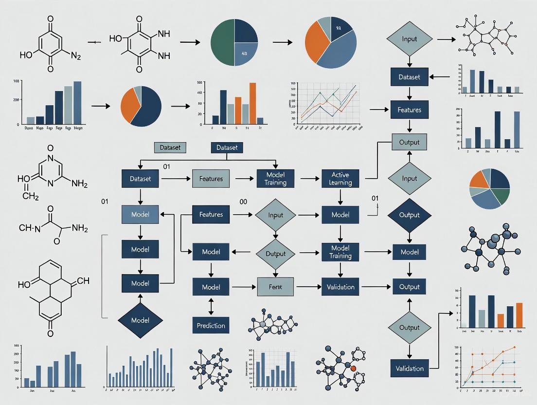
Diagram: The Active Learning Cycle. This workflow illustrates the iterative feedback loop of hypothesis generation, data query, and model refinement that defines AL in chemogenomics.
Detailed Experimental Protocol: An AL Case Study with FEgrow
The following protocol is adapted from a study that used AL to prioritize compounds from on-demand libraries targeting the SARS-CoV-2 main protease (Mpro) [5].
Objective
To efficiently search a combinatorial space of possible linkers and functional groups and identify synthesizable compounds with high predicted affinity for SARS-CoV-2 Mpro [5].
Materials and Reagents
Table: Essential Research Reagents and Tools for the FEgrow AL Protocol
| Item | Function/Description | Source/Example |
|---|---|---|
| Protein Structure | The 3D structure of the target protein used for pose optimization and scoring. | PDB ID 7BQY (SARS-CoV-2 Mpro with a bound fragment) [5] |
| Ligand Core | A fixed molecular fragment or known hit compound that serves as the base for growing new molecules. | A fragment from a crystallographic screen, placed in the binding pocket [5] |
| R-group & Linker Libraries | Libraries of chemical substituents and connecting units used to build new molecules from the core. | Distributed libraries with 2000+ linkers and 500+ R-groups [5] |
| FEgrow Software | Open-source package for building and optimizing ligands in a protein binding pocket. | https://github.com/cole-group/FEgrow [5] |
| gnina | A convolutional neural network scoring function used to predict binding affinity. | Integrated within the FEgrow workflow for scoring generated poses [5] |
| RDKit | Open-source cheminformatics toolkit used for molecular manipulation and conformer generation. | Used by FEgrow for merging, conformer generation, and filtering [5] |
| Machine Learning Model | A surrogate model trained on FEgrow outputs to predict scores for unscreened compounds. | A random forest model was used in the cited study [5] |
Step-by-Step Methodology
Initialization:
- Define the rigid protein structure, the ligand core, and the growth vector(s).
- Assemble the initial combinatorial library of linkers and R-groups.
Initial Sampling and Expensive Evaluation:
- Randomly select a small batch of (linker, R-group) combinations.
- Use FEgrow to build each full molecule into the protein binding pocket. This involves:
- Merging the core, linker, and R-group.
- Generating an ensemble of ligand conformers using RDKit's ETKDG algorithm.
- Filtering out conformers that clash with the protein.
- Optimizing the remaining conformers using a hybrid ML/MM potential energy function with a rigid protein [5].
- Score the resulting optimized poses using the gnina scoring function [5]. This score serves as the initial label (proxy for affinity) for the AL cycle.
Active Learning Loop:
- Train ML Model: Train a machine learning model (e.g., Random Forest) on the current set of evaluated molecules. The input features are representations of the (linker, R-group) pairs, and the target variable is the gnina score.
- Hypothesis & Query: Use the trained model to predict scores for all unevaluated molecules in the combinatorial library. Apply an acquisition function (e.g., selecting molecules with the highest predicted scores or those with high uncertainty) to select the next batch of promising candidates [5].
- Label: Run the selected batch of candidates through the FEgrow building and scoring pipeline (Step 2) to obtain their "expensive" gnina scores.
- Model Update: Add the newly evaluated molecules and their scores to the training set.
Termination and Validation:
- Repeat the AL loop for a predefined number of cycles or until model performance plateaus.
- Select the top-ranked molecules from the final cycle for purchase, synthesis, and experimental validation in a bioassay (e.g., a fluorescence-based Mpro activity assay) [5].
Integration with Broader Chemogenomics Workflows
The AL cycle is not an isolated process but is deeply integrated into modern chemogenomics and drug discovery pipelines. It is a key enabler of the Design-Build-Test-Learn (DBTL) cycle, where "Learn" directly corresponds to the model update and hypothesis steps in AL [2]. This integration is crucial for navigating complex biological fitness landscapes, which are characterized by high dimensionality, epistasis (non-additive mutational effects), and sparse regions of high fitness [2]. Furthermore, AL is increasingly combined with generative models in a symbiotic relationship. For instance, a Variational Autoencoder (VAE) can be embedded within nested AL cycles, where the generative model proposes novel molecules, and the AL cycle selects the most informative ones for expensive evaluation, using the results to fine-tune the generator [6]. This creates a powerful, self-improving system for de novo molecular design. The emerging paradigm of Human-in-the-Loop AL further enriches this workflow by incorporating feedback from chemistry experts to approve or refute model predictions, effectively acting as a cost-effective oracle to bridge gaps in training data and guide the exploration of chemical space [3].
The endeavor of drug discovery is fundamentally a search for a needle in a haystack, involving the exploration of an estimated 10^60 drug-like compounds to identify those with the desired therapeutic properties [8]. This vast chemical space presents an insurmountable challenge for traditional experimental methods, which can only screen a minuscule fraction of possible compounds due to constraints in time, cost, and resources. Furthermore, the acquisition of labeled data—molecules with experimentally determined properties—is exceptionally expensive and time-consuming, often requiring sophisticated laboratory techniques such as high-throughput screening, binding affinity assays, or toxicity tests. In this context, active learning (AL) has emerged as a powerful machine learning strategy that strategically addresses both the problem of vast chemical space and the scarcity of labeled data by iteratively selecting the most informative compounds for experimental validation, thereby accelerating the discovery process while significantly reducing costs [9] [8].
Active learning operates on a simple yet powerful premise: instead of randomly selecting compounds for testing, an AL algorithm proactively identifies which unlabeled data points would be most valuable to label, based on the current model's uncertainties or potential for improvement. This creates a human-in-the-loop paradigm where experimentalists guide both data collection and model training through targeted exploration within the vast chemical space [10]. The procedure adopts an iterative strategy of data collection, annotation, and training, using a specific set of rules to identify molecules that maximize the enhancement of model performance. By validating these molecules through wet lab experiments, active learning achieves greater improvements in model performance compared to random selection strategies, all within the same experimental annotation budget [10].
The Active Learning Workflow in Drug Discovery
Core Cycle and Implementation Strategies
The active learning framework follows an iterative cycle that integrates computational predictions with experimental validation. This process begins with a small initial set of labeled compounds used to train a preliminary machine learning model. The trained model then evaluates a much larger library of unlabeled compounds, scoring them based on a specific acquisition function. The most informative compounds are selected for experimental testing ("oracle" validation), and the newly acquired data is incorporated into the training set. The model is retrained with this expanded dataset, and the cycle repeats until a stopping criterion is met, such as achievement of target performance or exhaustion of resources [8] [10].
Figure 1: Active Learning Cycle for Drug Discovery
Several key strategies govern how compounds are selected at each iteration, balancing the exploration of diverse chemical space with the exploitation of promising regions [8] [11]:
- Greedy Selection: Chooses only the top predicted binders at every iteration step, focusing exclusively on exploitation.
- Uncertainty Sampling: Selects ligands for which the prediction uncertainty is largest, prioritizing exploration.
- Mixed Strategy: First identifies compounds with strong predicted binding affinity, then selects those with the most uncertain predictions among them, balancing exploitation and exploration.
- Narrowing Strategy: Combines broad selection in the first iterations with a subsequent switch to a greedy approach.
Quantitative Impact of Active Learning
The implementation of active learning strategies has demonstrated significant improvements in efficiency across multiple drug discovery applications. The following table summarizes key performance metrics reported in recent studies:
Table 1: Performance Metrics of Active Learning in Drug Discovery Applications
| Application Domain | Performance Improvement | Data Efficiency | Key Metrics | Citation |
|---|---|---|---|---|
| Mutagenicity Prediction | Competitive performance with small labeled samples | 57% reduction in training molecules required | Uncertainty-based sampling | [10] |
| Synergistic Drug Combinations | 60% of synergistic pairs found exploring only 10% of space | 82% savings in experimental materials | Precision-Recall AUC | [12] |
| Ultra-Large Library Docking | ~70% of top hits found at 0.1% of brute-force cost | 1000x cost reduction | Recall of top binders | [13] |
| Affinity Prediction (TYK2, USP7, D2R, Mpro) | Higher recall of top binders with sparse training data | Optimal batch size: 20-30 compounds | R², Spearman, F1 score | [11] |
Experimental Protocols and Methodologies
Protocol for Ligand Binding Affinity Optimization
A well-established AL protocol for optimizing ligand binding affinity involves multiple carefully designed steps that combine physics-based calculations with machine learning [8]:
Library Preparation: Generate an in silico compound library, typically through combinatorial expansion of R-groups around a core scaffold or by enumerating virtual compounds from available building blocks.
Initial Sampling: Employ weighted random selection for model initialization, where ligands are selected with probability inversely proportional to the number of similar ligands in the dataset. Similarity is determined using t-SNE embedding and 2D histogram binning.
Binding Pose Generation:
- For each ligand, identify the crystal structure with the highest Dice similarity based on RDKit topological fingerprint.
- Constrain coordinates of the largest substructure matches to the reference crystal structure.
- Generate initial guesses for remaining atoms via constrained embedding following the ETKDG algorithm.
- Refine ligand binding poses through hybrid topology molecular dynamics simulations in vacuum, morphing reference inhibitor into the ligand while lowering temperature.
Ligand Representation:
- Calculate molecular features including 2D descriptors (constitutional, electrotopological), 3D descriptors (molecular surface area), and molecular fingerprints (PLEC, MACCS).
- Generate interaction features including electrostatic and van der Waals interaction energies between ligand and each protein residue.
Active Learning Cycle:
- Train machine learning models (Gaussian Process, Random Forest, or Neural Networks) on current labeled set.
- Use selection strategy (mixed, uncertainty, or greedy) to choose the next batch of compounds for free energy calculations.
- Perform alchemical free energy calculations as the oracle for selected compounds.
- Incorporate newly labeled compounds into training set.
- Repeat for predetermined number of cycles or until performance convergence.
Protocol for Mutagenicity Prediction
The muTOX-AL framework demonstrates an effective AL approach for molecular mutagenicity prediction [10]:
Data Preparation:
- Curate mutagenicity dataset (e.g., TOXRIC with 7,495 compounds).
- Split data into five folds for cross-validation.
- For each fold, create initial labeled pool of 200 randomly selected samples, with remaining samples as unlabeled pool.
Feature Extraction:
- Generate molecular fingerprints (MACCS, Morgan) and molecular descriptors.
- Perform principal component analysis to visualize chemical space distribution.
Model Architecture:
- Implement feature extraction module for input processing.
- Design backbone module (neural network) for mutagenicity prediction.
- Incorporate uncertainty estimation module to quantify sample informativeness.
- Configure loss calculation module combining backbone and uncertainty losses.
Active Learning Cycle:
- Train model on current labeled pool.
- Calculate uncertainty scores for all samples in unlabeled pool.
- Select samples with highest uncertainty scores for oracle annotation.
- Add newly labeled samples to training set.
- Iterate until label budget exhausted or performance plateaus.
Successful implementation of active learning in drug discovery requires a combination of computational tools, molecular representations, and experimental assays. The following table details key resources mentioned in recent studies:
Table 2: Essential Research Reagents and Computational Tools for AL in Drug Discovery
| Tool/Resource | Type | Function in AL Pipeline | Examples/Implementation |
|---|---|---|---|
| Molecular Representations | Descriptors | Encode molecular structure for ML models | 2D/3D RDKit descriptors, Morgan fingerprints, MAP4, MACCS, PLEC fingerprints [8] [12] |
| Protein-Ligand Interaction Features | Descriptors | Capture binding site interactions | MedusaNet voxel grids, residue interaction energies, PLEC fingerprints [8] |
| AL Selection Algorithms | Software | Implement compound selection strategies | Mixed strategy, uncertainty sampling, greedy selection, BAIT, COVDROP, COVLAP [8] [14] |
| Free Energy Calculations | Computational Oracle | Provide accurate binding affinity predictions | Alchemical free energy calculations, FEP+ [8] [13] |
| Docking Tools | Computational Oracle | Screen large compound libraries | Glide docking, molecular docking scores [13] |
| Experimental Assays | Wet Lab Oracle | Validate computational predictions | Ames test (mutagenicity), binding assays (affinity), cell viability (synergy) [10] [12] |
| Cell Line Features | Descriptors | Incorporate cellular context in predictions | Gene expression profiles from GDSC database [12] |
Visualization of Selection Strategy Implementation
The implementation of different selection strategies follows specific logical pathways that determine how compounds are prioritized for experimental testing:
Figure 2: Compound Selection Strategies in Active Learning
Active learning represents a paradigm shift in computational drug discovery, directly addressing the fundamental challenges of vast chemical space and limited labeled data. By strategically selecting the most informative compounds for experimental validation, AL protocols achieve dramatic improvements in efficiency—reducing the number of required experiments by 57% in mutagenicity prediction [10], identifying 60% of synergistic drug combinations while exploring only 10% of combinatorial space [12], and recovering ~70% of top-scoring hits at 0.1% of the cost of exhaustive docking [13]. The continued refinement of molecular representations, selection strategies, and integration with high-performance computing and automated experimentation platforms will further solidify AL's role as an indispensable tool in modern drug discovery. As these methodologies become more sophisticated and widely adopted, they promise to significantly accelerate the identification of novel therapeutic compounds while reducing the substantial costs associated with traditional drug discovery approaches.
Active learning (AL) has emerged as a transformative paradigm in chemogenomics, enabling researchers to navigate the vast molecular and target interaction space with unprecedented efficiency. In the context of drug discovery, chemogenomics involves modeling the compound-protein interaction space to predict bioactivity, typically for identifying or optimizing drug candidates [15]. The core challenge AL addresses is the fundamental constraint of resources: wet-lab experiments, synthesis, and biological assays are notoriously time-consuming and expensive [3]. Active learning frameworks are strategically designed to overcome this by implementing an iterative, guided process for data acquisition. The two primary and interconnected objectives are: (1) Maximizing Information Gain: Each selected experiment should optimally reduce the uncertainty of the predictive model, enhancing its understanding of the structure-activity relationship across the chemical space. (2) Minimizing Experimental Cost: By prioritizing the most informative compounds for testing, AL aims to achieve high model performance and identify promising candidates with a minimal number of experiments, thereby de-risking and accelerating the project timeline [16] [17]. This guide details the technical implementation of these objectives, providing a roadmap for integrating AL into modern chemogenomics research.
Foundational Principles and Acquisition Strategies
The operationalization of AL's core objectives hinges on the deployment of specific acquisition functions—algorithms that score and rank unlabeled compounds based on their potential value to the model.
Core Acquisition Strategies
- Exploitation focuses on immediately improving the desired molecular property. This strategy selects compounds that the current model predicts will have the highest value (e.g., greatest potency, binding affinity, or other target property). While this can rapidly yield high-performing candidates, it risks converging on local optima and lacks chemical diversity [16].
- Exploration prioritizes the improvement of the model itself. It selects compounds where the model's predictive uncertainty is highest. By labeling these points, the model learns about previously poorly understood regions of the chemical space, expanding its applicability domain. This strategy can enhance the model's generalizability but may not directly yield the best compounds in the short term [3].
- Balanced Strategies combine exploration and exploitation to harness the benefits of both. A common framework is the Expected Predictive Information Gain (EPIG), which selects molecules expected to provide the greatest reduction in predictive uncertainty, leading to more accurate evaluations of subsequently generated molecules [3]. Another advanced balanced strategy is ActiveDelta, a paired-molecule approach that predicts the property improvement from the current best compound, directly guiding optimization while maintaining diversity [16].
Batch Active Learning for Practical Workflows
In real-world drug discovery, testing compounds one at a time is impractical. Batch Active Learning addresses this by selecting an optimal set of compounds for each experimental cycle. The key challenge is avoiding redundancy within a batch. Advanced methods like COVDROP and COVLAP select batches by maximizing the joint entropy (the log-determinant) of the epistemic covariance matrix of the batch predictions. This approach explicitly balances individual uncertainty (variance) and inter-compound diversity (covariance), preventing the selection of highly correlated candidates and ensuring the batch is collectively informative [17].
Table 1: Comparison of Key Active Learning Acquisition Strategies
| Strategy | Primary Objective | Key Mechanism | Advantages | Limitations |
|---|---|---|---|---|
| Exploitation | Find high-value compounds | Selects molecules with the highest predicted property value [16]. | Rapid identification of potent leads. | Can get stuck in local optima; low scaffold diversity. |
| Exploration | Improve model accuracy | Selects molecules with the highest predictive uncertainty [3]. | Broadens model knowledge; improves generalizability. | May not directly advance primary optimization goal. |
| EPIG | Reduce predictive uncertainty | Maximizes the expected information gain for model predictions [3]. | Balances exploration and exploitation; improves predictor accuracy. | Computationally intensive. |
| ActiveDelta | Guide molecular optimization | Predicts property improvements via molecular pairing [16]. | Effective with small data; identifies diverse scaffolds. | Requires paired data representation. |
| Batch Selection (COVDROP) | Maximize batch information | Maximizes joint entropy of batch predictions [17]. | Practical for HTS; ensures diversity within a batch. | High computational complexity for large candidate pools. |
Practical Implementation and Workflows
Translating AL theory into practice requires a structured workflow and an understanding of the supporting computational infrastructure.
The Human-in-the-Loop (HITL) Framework
A powerful extension of AL integrates domain expertise directly into the loop. In this framework, a property predictor (e.g., a QSAR model) guides the generative design of molecules. An acquisition function like EPIG then identifies generated molecules that are most informative for the predictor—often those with high predicted scores but also high uncertainty. Instead of immediate wet-lab testing, these molecules are evaluated by human experts who can approve or refute the predicted properties based on their domain knowledge. This feedback is used to refine the property predictor, creating a closed-loop system that leverages human insight to efficiently navigate the chemical space and generate molecules that are both promising and synthetically tractable [3].
The FEgrow-AL Workflow for Structure-Based Design
A concrete example of an AL-driven workflow is demonstrated by the FEgrow software for de novo drug design. This workflow targets a specific protein binding pocket:
- Input: A fixed ligand core and libraries of linkers and functional groups (R-groups) are defined.
- Building & Scoring: FEgrow builds the full ligand in the protein pocket, optimizes its pose, and scores it using a function like the gnina CNN scoring function to predict binding affinity.
- Active Learning Cycle:
- An initial subset of compounds is built and scored.
- This data trains a machine learning model (e.g., a random forest or neural network) to predict the objective function (e.g., docking score) for the entire combinatorial space.
- The model selects the next most promising batch of compounds (e.g., those with the best-predicted scores) for evaluation with the expensive FEgrow process.
- The cycle repeats, iteratively improving the model and focusing resources on the most valuable regions of the chemical space [5].
Table 2: Essential Research Reagent Solutions for an AL-Driven Campaign
| Reagent / Tool Category | Specific Examples | Function in the AL Workflow |
|---|---|---|
| Cheminformatics Libraries | RDKit [5] [16], DeepChem [17] | Handles molecular I/O, fingerprint generation (e.g., Morgan fingerprints), and descriptor calculation. |
| Molecular Representations | Morgan Fingerprints (ECFP) [16], SMILES/SELFIES [18], Graph Neural Networks [17] | Encodes molecular structure for machine learning models. |
| Predictive & Generative Models | Chemprop (D-MPNN) [16], XGBoost [16], Generative Adversarial Networks (GANs) [19] | Serves as the surrogate model for property prediction or generates novel molecular structures. |
| Active Learning & Optimization Packages | FEgrow [5], BATCHIE [20], Custom implementations of COVDROP/COVLAP [17] | Orchestrates the active learning cycle, including model training, candidate ranking, and batch selection. |
| Experimental Assay Platforms | High-Throughput Screening (HTS) [21], Fluorescence-based bioassays [5] | Functions as the "oracle" to provide experimental validation and ground-truth labels for selected compounds. |
Case Studies and Experimental Validation
Retrospective and prospective validations across diverse domains underscore the real-world impact of AL in achieving its core objectives.
Small Molecule Optimization with ActiveDelta
In a benchmark study across 99 Ki datasets from ChEMBL, the ActiveDelta strategy was pitted against standard exploitative AL. ActiveDelta, which uses paired molecular representations to predict potency improvements, consistently outperformed standard methods. It identified a greater number of the most potent inhibitors and, critically, achieved this with enhanced chemical diversity as measured by Murcko scaffold analysis. This demonstrates that AL can simultaneously minimize experimental effort (by requiring fewer cycles to find potent hits) and maximize information gain (by exploring a broader chemical space) [16].
Large-Scale Combination Screening with BATCHIE
Screening for effective drug combinations faces a combinatorial explosion of possibilities. The BATCHIE platform uses a Bayesian active learning approach based on Probabilistic Diameter-based Active Learning (PDBAL) to design maximally informative batches of combination experiments. In a prospective screen of a 206-drug library across 16 pediatric cancer cell lines, BATCHIE accurately predicted unseen drug combinations and detected synergies after exploring only 4% of the 1.4 million possible experiments. This dramatic reduction in experimental cost was achieved without sacrificing information gain, as the model successfully identified a panel of effective combinations, including a clinically relevant hit [20].
In Vitro Protein Production Optimization
Beyond drug discovery, AL's principles are universally applicable. In one study, researchers sought to optimize a cell-free buffer system for protein production—a combinatorial space of over 4 million possible compositions. An AL strategy using an ensemble of neural networks and a balanced acquisition function achieved a 34-fold increase in protein yield after testing only ~1000 compositions. Furthermore, they demonstrated that a minimal set of 20 highly informative compositions was sufficient to train a model that could accurately predict optimal buffers for new lysates, showcasing a powerful "one-step" optimization method with minimal experimental overhead [22].
Table 3: Summary of Experimental Outcomes from AL Case Studies
| Case Study | Domain | Key AL Method | Reported Efficiency Gain | Performance Improvement |
|---|---|---|---|---|
| ActiveDelta [16] | Ki Potency Prediction | Molecular Pairing & Exploitation | Identified more potent and diverse inhibitors with the same data budget. | Superior performance in identifying top-potency compounds compared to standard AL. |
| BATCHIE [20] | Combination Drug Screening | Probabilistic Diameter-based AL (PDBAL) | Screened only 4% of a 1.4M-experiment space. | Accurately predicted unseen combinations; identified validated synergistic hits. |
| Cell-Free Optimization [22] | Bioprocessing | Ensemble Neural Networks | Achieved optimization after testing ~0.02% of search space. | 34-fold increase in protein production yield. |
| FEgrow [5] | Structure-Based Design | Model-based Batch Selection | Enabled efficient search of combinatorial linker/R-group space. | Identified purchasable compounds with activity against SARS-CoV-2 Mpro. |
Experimental Protocols and Best Practices
Protocol: Implementing an Exploitative ActiveDelta Cycle
This protocol is adapted from the benchmark study detailed in [16].
Initialization:
- Begin with a small, randomly selected set of labeled compounds (e.g., N=2) as the initial training data.
- Define a large pool of unlabeled compounds as the learning set.
Model Training (ActiveDelta):
- Pre-process the training data by creating all possible pairwise combinations of molecules.
- For each pair (A, B), calculate the difference in the target property (e.g., ΔKi = Ki,B - Ki,A).
- Train a machine learning model (e.g., the two-molecule version of Chemprop or a paired-fingerprint XGBoost) on these pairs to predict the property difference.
Candidate Selection:
- Identify the single best compound (e.g., lowest Ki) in the current training set. Designate this as the reference molecule.
- Pair this reference molecule with every compound in the unlabeled learning set.
- Use the trained ActiveDelta model to predict the property improvement (Δ) for each of these pairs.
- Select the compound from the learning set that is part of the pair with the highest predicted improvement.
Iteration:
- The selected compound is experimentally tested ("labeled") and added to the training dataset.
- The model is retrained on the expanded and re-paired training data.
- The cycle (Steps 2-4) repeats until the experimental budget is exhausted or a performance target is met.
Protocol: Setting Up a Batch AL Campaign with COVDROP
This protocol is based on the methodology described in [17].
Problem Formulation:
- Assemble a large pool of unlabeled molecules (e.g., from a virtual library).
- Define a batch size B (e.g., 30 molecules) appropriate for your experimental throughput.
Model and Uncertainty Setup:
- Choose a deep learning model (e.g., a Graph Neural Network) suitable for regression/classification of your molecular property.
- Implement an uncertainty quantification technique. For COVDROP, this is typically Monte Carlo (MC) Dropout.
- During inference, perform multiple forward passes (e.g., 100) with dropout enabled.
- The predictions from these passes form a distribution for each molecule.
Covariance Matrix Calculation:
- For all molecules in the unlabeled pool, compute the predictive covariance matrix, C.
- Each element Cij represents the covariance between the predictive distributions of molecule i and molecule j. This captures both individual uncertainties (variances, Cii) and similarities between molecules (covariances, C_ij).
Greedy Batch Selection:
- Initialize an empty batch.
- Iteratively, for k = 1 to B:
- Find the molecule in the unlabeled pool that, when added to the current batch, maximizes the log-determinant of the resulting batch's covariance submatrix, CB.
- This step seeks to maximize the joint entropy (total information content) of the batch.
- The final set of B selected molecules constitutes the optimal batch.
Experimental Cycle:
- The selected batch is tested experimentally.
- The model is retrained on the newly labeled data.
- The process repeats from Step 3 for the next batch.
Active learning represents a fundamental shift in the approach to computational and experimental research in chemogenomics. By strategically prioritizing data acquisition, it directly attacks the core bottlenecks of cost and time. Frameworks like Human-in-the-Loop AL, ActiveDelta, and BATCHIE provide concrete methodologies to simultaneously maximize information gain and minimize experimental cost. The resulting models are not only more predictive and robust but also guide the exploration of chemical space more intelligently, leading to the discovery of potent, diverse, and novel candidates with a fraction of the traditional resource investment. As these methodologies continue to mature and integrate with cutting-edge generative AI, they are poised to become the standard operating procedure for efficient and effective drug discovery.
In chemogenomics, where researchers model the complex interactions between chemical compounds and biological targets, the quality of training data is a primary determinant of machine learning (ML) model success. The field consistently grapples with two pervasive data flaws: severe imbalance and significant redundancy. Bioactivity datasets often exhibit extreme skewness, with hit rates in high-throughput screens sometimes as low as 0.01%, creating a massive imbalance between active and inactive compounds [23]. Simultaneously, chemical libraries frequently contain clusters of structurally similar compounds, introducing redundancy that biases models and wastes computational resources. These flaws lead to ML models that appear accurate yet fail to predict the biologically important minority class (e.g., active compounds) and generalize poorly to novel chemical scaffolds.
Active learning (AL) has emerged as a powerful computational strategy to address these intrinsic data problems. AL is an iterative feedback process that intelligently selects the most informative data points for labeling and model training [1]. By prioritizing informative instances over redundant ones and strategically addressing class imbalance through intelligent sampling, AL enables the construction of highly predictive models from smaller, higher-quality datasets. Within chemogenomics, this capability allows researchers to extract maximum value from expensive experimental data, accelerating the identification of novel compound-target interactions while minimizing resource expenditure [15].
How Active Learning Tackles Data Flaws
Core Mechanisms Against Data Imbalance
Active learning counteracts data imbalance through its fundamental operating principle: uncertainty sampling. Instead of training models on entire available datasets, AL begins with a small initial training set and iteratively selects the most uncertain instances for experimental validation and inclusion in subsequent training cycles [23]. This approach automatically guides the sampling process toward the decision boundary where the model struggles most to distinguish between classes, which naturally leads to increased representation of the minority class in the training data.
Research demonstrates that this adaptive subsampling strategy significantly outperforms both training on complete datasets and using static subsampling methods. In studies across multiple molecular classification tasks, AL-based subsampling achieved performance improvements of up to 139% in Matthews Correlation Coefficient compared to models trained on full datasets [23]. The strategy proves particularly robust against label noise, maintaining performance even when significant portions of the training data contain errors, a common issue in experimental biological data.
Strategic Approaches to Reduce Redundancy
To address data redundancy, AL incorporates diversity criteria into its selection algorithms. Rather than selecting batches of compounds based solely on individual uncertainty, advanced AL methods choose sets of compounds that are collectively informative. These approaches maximize the coverage of the chemical space within each batch, ensuring that each selected compound provides unique information to the model.
Batch active learning methods specifically tackle this challenge by selecting compounds that are both uncertain and diverse. One approach uses covariance matrices to quantify the similarity between unlabeled samples, then selects batches that maximize the joint entropy (information content) by maximizing the determinant of the covariance submatrix [17]. This ensures selected compounds are non-redundant and collectively provide the maximum possible information gain, effectively eliminating the bias introduced by structurally similar compound clusters in traditional screening libraries.
Active Learning Methodologies in Practice
Workflow and Implementation
The practical implementation of active learning in chemogenomics follows a structured, iterative cycle that integrates computational modeling with experimental validation. The standard AL workflow comprises several key stages that form a closed feedback loop, continuously refining the model with each iteration.
Diagram 1: Standard AL workflow for chemogenomics. This iterative process efficiently builds predictive models by strategically selecting the most informative compounds for experimental testing.
The process begins with a small initial training set of compound-target interactions, which may be randomly selected or chosen for diversity. A predictive model (e.g., random forest, neural network) is trained on this initial data. The trained model then evaluates all compounds in the unlabeled pool, estimating the uncertainty of each prediction. The most informative compounds are selected based on predefined criteria (typically combining uncertainty and diversity metrics) for experimental validation. The newly acquired experimental data is incorporated into the training set, and the model is retrained. This cycle continues until a stopping criterion is met, such as performance plateau or exhaustion of resources [1] [23].
Key Acquisition Functions for Data Selection
Acquisition functions form the mathematical core of AL systems, determining which data points are selected in each iteration. The table below summarizes the primary acquisition strategies used to combat data flaws in chemogenomics.
Table 1: Acquisition Functions for Addressing Data Flaws in Chemogenomics
| Function Type | Mechanism | Addresses | Advantages | Limitations |
|---|---|---|---|---|
| Uncertainty Sampling | Selects instances where model prediction is most uncertain | Data imbalance | Targets decision boundary; improves minority class detection | May select outliers; ignores diversity |
| Diversity Sampling | Maximizes dissimilarity between selected instances | Data redundancy | Broadly explores chemical space; reduces redundancy | May include clearly unproductive regions |
| Query-by-Committee | Selects instances with most disagreement between ensemble models | Data imbalance | Robust uncertainty estimation; reduces model bias | Computationally intensive for large ensembles |
| Expected Model Change | Selects instances causing greatest model change | Both | High information per sample; efficient learning | Computationally expensive; complex implementation |
| Batch BALD | Maximizes mutual information between batch and model parameters | Both | Optimizes batch diversity and uncertainty | High computational complexity for large batches |
In practice, advanced AL implementations often combine multiple strategies. For example, deep batch active learning methods use covariance matrices to select compounds that maximize joint entropy, simultaneously addressing both uncertainty and diversity [17]. Similarly, the "balanced-diverse" approach applies both class balancing and structural diversity criteria to create optimal training subsets [23].
Experimental Protocols and Benchmarking
Implementing AL in chemogenomics requires careful experimental design and rigorous benchmarking. The following protocol outlines a standardized approach for AL implementation in compound-target interaction prediction:
Initial Setup and Data Preparation
- Dataset Collection: Compile a comprehensive dataset of compound-target interactions, ensuring representation of both active and inactive classes. Public databases like ChEMBL are commonly used sources.
- Representation: Encode molecular structures using appropriate representations. Morgan fingerprints (radius 2, 1024 bits) implemented in RDKit provide a robust baseline representation [23].
- Splitting: Perform a 50:50 scaffold split to separate compounds into training and validation sets, ensuring structurally distinct sets for rigorous evaluation.
Active Learning Implementation
- Initialization: Randomly select one positive and one negative example from the training pool to form the initial training set.
- Model Training: Train a predictive model (e.g., Random Forest with 100 trees and Gini impurity) on the current training set.
- Uncertainty Quantification: Apply ensemble-based uncertainty estimation by calculating variance in prediction probabilities across all trees in the Random Forest.
- Compound Selection: Identify the compound with the highest predictive uncertainty from the unlabeled pool.
- Iteration: Add the selected compound to the training set and retrain the model. Repeat steps 3-5 until all compounds are exhausted or performance plateaus.
- Evaluation: Monitor performance metrics (Matthews Correlation Coefficient, F1 score, balanced accuracy) on the independent validation set throughout the process.
This protocol has demonstrated consistent success across multiple bioactivity prediction tasks, typically achieving peak performance with only 10-25% of the total data available [15] [23].
Performance Benchmarks and Comparative Analysis
Rigorous benchmarking studies demonstrate the significant advantages of AL approaches over conventional screening and random selection strategies. The performance gains are consistent across diverse drug discovery tasks, from virtual screening to molecular property prediction.
Table 2: Performance Benchmarking of Active Learning Methods in Drug Discovery
| Application Domain | Dataset | Best Performing AL Method | Performance Gain vs. Random | Data Efficiency |
|---|---|---|---|---|
| Virtual Screening | Protein-Ligand Affinity | Covariance Dropout (COVDROP) | ~40% higher hit rate | Reaches maximum performance with 50% less data |
| Molecular Property Prediction | Aqueous Solubility | Batch Active Learning with Diversity | 30% lower RMSE | 60% fewer samples needed for same accuracy |
| Compound-Target Interaction | HIV Replication Inhibition | Ensemble-based Uncertainty Sampling | 139% higher MCC | Identifies 80% of actives with only 20% of total data |
| Toxicity Prediction | Clinical Trial Toxicity | Balanced-Diverse Sampling | 45% higher F1 score | Achieves peak performance with 25% of data |
The consistency of these results across different domains highlights the robustness of AL approaches to the data flaws prevalent in chemogenomics. Notably, AL not only achieves better final performance but does so with substantially less experimental effort, directly addressing the resource constraints common in drug discovery programs.
Advanced Implementations and Future Directions
Integration with Generative Models
Recent advances combine AL with generative artificial intelligence to create more powerful molecular design pipelines. One innovative approach integrates a variational autoencoder (VAE) with two nested AL cycles [6]. In this architecture, the VAE generates novel molecular structures, while the AL components iteratively select the most promising candidates for evaluation using both chemoinformatic predictors (drug-likeness, synthetic accessibility) and physics-based oracles (molecular docking). This synergistic combination addresses fundamental limitations of generative models, including poor target engagement and limited synthetic accessibility, while simultaneously exploring novel regions of chemical space.
This VAE-AL framework has demonstrated impressive experimental validation. When applied to CDK2 inhibitor design, the approach generated novel molecular scaffolds distinct from known inhibitors, with 8 out of 9 synthesized molecules showing biological activity, including one with nanomolar potency [6]. This success highlights how AL can guide generative models toward chemically feasible, biologically active compounds while navigating around data scarcity and quality issues.
The Scientist's Toolkit: Essential Research Reagents
Successful implementation of AL in chemogenomics relies on a core set of computational tools and resources. The table below summarizes key components of the AL research toolkit.
Table 3: Essential Research Reagents for AL Implementation in Chemogenomics
| Tool/Resource | Type | Function | Application in AL Workflow |
|---|---|---|---|
| RDKit | Cheminformatics Library | Molecular representation and manipulation | Generates molecular fingerprints (e.g., Morgan fingerprints) for compound encoding |
| DeepChem | Deep Learning Library | Molecular machine learning | Provides implementations of graph neural networks for compound property prediction |
| scikit-learn | Machine Learning Library | General-purpose ML algorithms | Supplies Random Forest and other classifiers with uncertainty estimation capabilities |
| GPy | Gaussian Process Library | Probabilistic non-parametric models | Offers built-in uncertainty quantification for regression tasks |
| ChemBL Database | Bioactivity Database | Repository of compound-target interactions | Sources initial training data and provides ground truth for experimental validation |
| BAIT | Batch AL Implementation | Fisher information-based selection | Optimizes batch selection for deep learning models |
| GeneDisco | AL Benchmarking Suite | Benchmarking platform for AL algorithms | Evaluates and compares different AL strategies on standardized tasks |
Emerging Trends and Future Outlook
The future of AL in chemogenomics points toward increased integration with experimental automation and more sophisticated uncertainty quantification techniques. As noted in recent research, "AL-assisted design-build-test-learn cycles can quickly converge on the true landscape with just a few iterations of small-scale sampling, filtering out a significant portion of unnecessary, costly, and time-consuming validations" [2]. This is particularly valuable in genetic engineering and protein design applications, where experimental throughput continues to increase.
Future developments will likely focus on multi-objective optimization AL, which simultaneously balances multiple molecular properties (efficacy, selectivity, pharmacokinetics), and transfer AL, which leverages knowledge from related targets to jumpstart learning for novel targets with limited data [1]. Additionally, the integration of AL with foundation models pre-trained on large chemical libraries represents a promising direction for few-shot learning in chemogenomics, potentially further reducing the experimental burden required for model development.
Active learning provides a powerful, principled framework for addressing the fundamental data quality challenges—imbalance and redundancy—that persistently hamper traditional approaches in chemogenomics. By intelligently selecting the most informative compounds for experimental testing, AL systems systematically build balanced, representative training datasets that maximize predictive performance while minimizing resource expenditure. The robust performance gains demonstrated across diverse drug discovery applications, from virtual screening to molecular generation, underscore the transformative potential of AL methodologies. As chemogenomics continues to grapple with increasingly complex research questions and expanding chemical spaces, the strategic integration of active learning into the research workflow will be essential for extracting meaningful insights from imperfect data and accelerating the discovery of novel therapeutic agents.
Active Learning in Action: Key Applications from Virtual Screening to Molecule Generation
The identification of novel compound-protein interactions is a fundamental objective in drug discovery. Traditional virtual screening methods, which rely on the exhaustive computational docking of every molecule in a large virtual library, are becoming increasingly prohibitive as these libraries now routinely contain billions of compounds [24]. This creates a critical bottleneck in the early stages of drug development. Within this context, active learning has emerged as a powerful machine learning framework to dramatically increase the efficiency of virtual screening campaigns. As a core methodology in computational chemogenomics—which aims to model the compound-protein interaction space—active learning enables the construction of highly predictive models by iteratively selecting the most informative ligand-target interactions for evaluation [15]. This technical guide explores the application of active learning to structure-based virtual screening, providing a detailed examination of its performance, methodologies, and implementation to help researchers prioritize the most promising compounds for experimental testing.
Active Learning Performance and Quantitative Benchmarks
Active learning guided virtual screening has demonstrated remarkable efficiency in identifying top-scoring compounds from ultra-large libraries by evaluating only a small fraction of the total collection. The performance can be quantified using the Enrichment Factor (EF), which measures the ratio of the percentage of top-k scores found by the model-guided search to the percentage found by a random search [24]. The following table summarizes key performance metrics from recent studies:
Table 1: Performance Benchmarks of Active Learning in Virtual Screening
| Virtual Library Size | Surrogate Model | Acquisition Function | Screening Effort | Top Compounds Identified | Reference |
|---|---|---|---|---|---|
| 100 million compounds | Directed-Message Passing Neural Network (D-MPNN) | Upper Confidence Bound (UCB) | 2.4% | 94.8% of top-50,000 | [24] |
| 100 million compounds | Directed-Message Passing Neural Network (D-MPNN) | Greedy | 2.4% | 89.3% of top-50,000 | [24] |
| 99.5 million compounds | Pretrained Transformer / Graph Neural Network | Bayesian Optimization | 0.6% | 58.97% of top-50,000 | [25] |
| 10,560 compounds | Feedforward Neural Network | Greedy | 6.0% | 66.8% of top-100 (EF=11.9) | [24] |
| 10,560 compounds | Random Forest | Greedy | 6.0% | 51.6% of top-100 (EF=9.2) | [24] |
Beyond standard docking, the ActiveDelta approach, which leverages paired molecular representations to predict property improvements, has shown superior performance in exploitative active learning. In benchmarks across 99 Ki datasets, ActiveDelta implementations (using both Chemprop and XGBoost) consistently identified a greater number of potent inhibitors and achieved higher scaffold diversity compared to standard active learning methods [26].
Key Components of an Active Learning Workflow for Virtual Screening
An effective active learning system for virtual screening integrates several key components, each of which must be carefully selected based on the specific campaign goals.
Table 2: Key Components of an Active Learning Workflow
| Component | Description | Common Options & Examples |
|---|---|---|
| Surrogate Model | A machine learning model trained on docking results to predict scores of unscreened compounds. | - Random Forest (RF): Fast, works well on small data. [24]- Feedforward Neural Network (NN): Improved performance over RF. [24]- Message Passing Neural Network (MPNN): State-of-the-art, captures graph structure. [24] [26]- Pretrained Models (Transformer/GNN): High sample efficiency. [25] |
| Acquisition Function | The strategy for selecting the next compounds to dock based on the surrogate model's predictions. | - Greedy: Selects compounds with the best-predicted score. [24]- Upper Confidence Bound (UCB): Balances prediction (exploitation) and uncertainty (exploration). [24]- Thompson Sampling (TS): Selects based on stochastic predictions from a probabilistic model. [24] |
| Objective Function | The expensive, physics-based calculation that the surrogate model approximates. | - Docking Score (e.g., AutoDock Vina, Glide, RosettaVS): Primary metric for binding affinity. [24] [13] [27]- Free Energy Perturbation (FEP+): Higher accuracy binding affinity prediction. [13]- Composite Scores: Can include other properties like molecular weight or specific protein-ligand interactions. [5] |
The Active Learning Cycle
The integration of these components forms an iterative cycle, as illustrated in the following workflow:
Experimental Protocols and Case Studies
Protocol 1: Bayesian Optimization with D-MPNN for Ultra-Large Libraries
This protocol, detailed by Graff et al. [24], is designed for screening libraries containing tens to hundreds of millions of compounds.
- Library Preparation: Obtain the virtual compound library (e.g., ZINC, Enamine REAL). Standardize structures and generate 3D conformers.
- Initialization: Randomly select a small initial batch of compounds (e.g., 0.1% of the library) and dock them using a program like AutoDock Vina to establish an initial training set.
- Model Training: Train a Directed-Message Passing Neural Network (D-MPNN) as the surrogate model on the accumulated docking scores. The D-MPNN operates directly on the molecular graph, learning meaningful features for prediction [24] [26].
- Acquisition and Selection:
- Use the trained model to predict the docking scores and associated uncertainties for all remaining compounds in the library.
- Apply an acquisition function, such as the Upper Confidence Bound (UCB), to select the next batch of compounds. UCB is defined as ( \text{UCB}(x) = \mu(x) + \kappa \sigma(x) ), where ( \mu(x) ) is the predicted score, ( \sigma(x) ) is the uncertainty, and ( \kappa ) is a parameter balancing exploration and exploitation [24].
- Iteration: Dock the newly selected batch, add the results to the training data, and retrain the model. Repeat steps 3-5 until a predefined budget is exhausted or performance plateaus.
- Output: The top-scoring compounds identified across all iterations are prioritized for experimental testing.
Protocol 2: ActiveDelta for Potency Optimization in Low-Data Regimes
The ActiveDelta protocol is particularly effective in early project stages with limited data, as it focuses on predicting relative improvements rather than absolute binding scores [26].
- Data Pairing: Start with a small training set of compounds with known binding affinities (e.g., Ki values). Create a paired dataset where each data point consists of two molecules and the difference in their potency.
- Model Training: Train a machine learning model (e.g., a paired D-MPNN in Chemprop or a paired-fingerprint XGBoost) on this paired dataset. The model learns to predict the potency difference between any two molecules [26].
- Acquisition and Selection:
- Identify the most potent molecule, ( M{best} ), in the current training set.
- For every molecule ( Mi ) in the learning pool, form a pair ( (M{best}, Mi) ).
- Use the trained model to predict the potency improvement for ( Mi ) relative to ( M{best} ).
- Select the compound with the largest predicted improvement for the next round of experimental testing or computational evaluation.
- Iteration: The newly tested compound is added to the training set, and all possible new pairs are generated for the next round of model training and selection.
Case Study: Targeting SARS-CoV-2 Mpro with FEgrow and Active Learning
A recent study by Cree et al. [5] successfully integrated active learning with the FEgrow software to design inhibitors for the SARS-CoV-2 main protease (Mpro).
- Objective: To efficiently search a combinatorial space of linkers and R-groups grown from a fixed ligand core.
- Workflow: The FEgrow software was used to build and score ligands in the protein binding pocket using a hybrid ML/MM potential. An active learning cycle was implemented where a machine learning model was trained on a subset of FEgrow results and then used to select the most promising compounds for the next evaluation round [5].
- Integration with On-Demand Libraries: The chemical space was "seeded" with purchasable compounds from the Enamine REAL database, ensuring synthetic tractability.
- Outcome: The workflow identified several novel designs, some of which showed high similarity to known inhibitors from the COVID Moonshot effort. Prospective testing of 19 purchased compounds yielded three with weak activity, validating the approach for hit identification [5].
The Scientist's Toolkit: Essential Research Reagents and Software
Table 3: Key Software Tools for Active Learning Virtual Screening
| Tool Name | Type/Function | Key Features | Reference/Link |
|---|---|---|---|
| MolPAL | Open-source active learning software | Implements various surrogate models (RF, NN, MPNN) and acquisition functions (Greedy, UCB, TS). | [24] |
| FEgrow | Open-source tool for building congeneric series | Grows ligands in protein pockets, integrates with active learning, uses hybrid ML/MM for optimization. | [5] |
| ActiveDelta | Algorithm for exploitative active learning | Uses paired molecular representations to predict property improvements; available in Chemprop. | [26] |
| Schrödinger Active Learning Applications | Commercial platform | Active Learning Glide for docking and Active Learning FEP+ for free energy calculations. | [13] |
| OpenVS | Open-source AI-accelerated virtual screening platform | Integrates RosettaVS docking with active learning for screening billion-member libraries. | [27] |
| AutoDock Vina | Molecular docking software | Fast, widely used docking engine for generating initial training data. | [24] |
| gnina | Docking with convolutional neural networks | Used as a scoring function within workflows like FEgrow. | [5] |
Active learning represents a paradigm shift in how computational scientists approach the vastness of chemical space in drug discovery. By strategically guiding the selection of compounds for expensive virtual screening evaluations, active learning frameworks can recover the vast majority of top-performing hits at a fraction of the computational cost of exhaustive screens. As virtual libraries continue to expand into the billions, the adoption of these intelligent, adaptive methodologies will be crucial for maintaining efficiency in chemogenomics research. The continued development of more accurate surrogate models, such as pretrained transformers and advanced graph neural networks, along with innovative acquisition strategies like ActiveDelta, promises to further enhance the sample efficiency and effectiveness of virtual screening campaigns, ultimately accelerating the delivery of new therapeutic compounds.
Predicting Drug-Target Interactions (DTIs) in a Multi-Target Paradigm
The drug discovery process is notoriously complex, expensive, and time-consuming, typically costing approximately $2.6 billion and taking over 10 years from concept to market approval [28]. A fundamental challenge in this process is efficiently identifying interactions between drugs and their protein targets within an enormous chemical and biological space. Chemogenomics has emerged as a powerful framework that aims to model the entire compound-protein interaction space systematically, rather than focusing on individual targets in isolation [15] [29]. This paradigm recognizes that pharmacological compounds often interact with multiple targets, and leveraging these polypharmacological relationships can accelerate drug discovery and repositioning efforts.
Active Learning (AL) represents a transformative approach within computational chemogenomics. As an iterative, feedback-driven machine learning process, AL strategically selects the most informative data points for labeling and model training [1]. This methodology is particularly valuable in drug discovery contexts where obtaining labeled data (experimentally confirmed drug-target interactions) is both costly and time-intensive. By focusing resources on collecting the most valuable data, active learning enables the construction of highly predictive models using only 10-25% of large bioactivity datasets, dramatically reducing experimental requirements while maintaining model accuracy [15].
Active Learning Fundamentals in Chemogenomics
Core Conceptual Framework
Active learning operates on the principle that a machine learning algorithm can achieve greater accuracy with fewer training labels if it is allowed to choose which data points to learn from. In the context of drug-target interaction prediction, this translates to an iterative process where the model selectively identifies which compound-target pairs should be prioritized for experimental testing to maximally improve model performance [1].
The fundamental AL cycle consists of four key phases:
- Initial Model Training: A base model is trained on a small set of labeled drug-target interactions
- Query Strategy Application: The model evaluates unlabeled instances and selects the most informative ones according to a predefined acquisition function
- Experimental Labeling: The selected compound-target pairs are tested experimentally (e.g., via high-throughput screening)
- Model Update: Newly labeled data is incorporated into the training set, and the model is retrained
This process repeats until a stopping criterion is met, such as performance convergence or exhaustion of experimental resources [1] [17].
Algorithmic Approaches and Query Strategies
Several algorithmic approaches have been developed for active learning in chemogenomics:
Query-by-Committee employs multiple models (a committee) to evaluate unlabeled instances. Structures with high disagreement among committee members are selected for labeling, as this disagreement indicates model uncertainty and potential learning value [30]. This approach has been successfully used to create diverse datasets like QDπ, which incorporates 1.6 million molecular structures while maximizing chemical diversity [30].
Uncertainty Sampling selects instances where the model's prediction confidence is lowest. For regression tasks (e.g., predicting binding affinity), this may involve selecting compounds with highest predictive variance [17].
Representation-based Methods focus on selecting diverse compounds that cover the chemical space efficiently. K-means clustering and related approaches ensure broad coverage of the molecular feature space [17].
Table 1: Common Active Learning Query Strategies in DTI Prediction
| Strategy | Mechanism | Advantages | Limitations |
|---|---|---|---|
| Greedy Acquisition | Selects compounds with highest predicted activity | Simple, computationally efficient; effective for molecular docking [31] | May get stuck in local optima; poor exploration |
| Uncertainty Sampling | Selects compounds with highest prediction uncertainty | Directly addresses model uncertainty; good for error reduction [1] | Sensitive to initial model bias |
| Upper Confidence Bound (UCB) | Balances prediction score and uncertainty | Balanced exploration-exploitation trade-off [31] | Requires tuning of balance parameter |
| Query-by-Committee | Selects compounds with highest committee disagreement | Robust; reduces model-specific bias [30] | Computationally intensive; requires multiple models |
| Diversity Sampling | Maximizes chemical space coverage | Ensures broad exploration [17] | May miss high-activity regions |
Experimental Design and Methodologies
Workflow Implementation
Implementing active learning for DTI prediction requires careful orchestration of computational and experimental components. The following workflow visualization captures the iterative nature of this process:
Active Learning Workflow for DTI Prediction
Protocol Details: QDπ Dataset Construction
The creation of the QDπ dataset exemplifies rigorous active learning implementation for chemogenomic modeling [30]. The methodology employed four distinct strategies for incorporating molecular structures:
Direct Inclusion: Source databases with energies and forces already calculated at the ωB97M-D3(BJ)/def2-TZVPPD theory level were incorporated entirely.
Relabeling: Small databases without reference-level data were recalculated at the target theory level without geometry reoptimization.
Active Learning Pruning: For large databases, a query-by-committee approach identified non-redundant structures. The active learning cycle involved:
- Training 4 independent machine learning potential models with different random seeds
- Calculating energy and force standard deviations between models for each structure
- Setting thresholds of 0.015 eV/atom for energy and 0.20 eV/Å for force standard deviations
- Selecting up to 20,000 candidate structures per cycle exceeding these thresholds
- Terminating when all structures were either included or excluded [30]
Active Learning Extension: For small databases containing only optimized structures, molecular dynamics sampling was combined with active learning to identify thermally accessible conformations.
Protocol Details: EviDTI Framework
The EviDTI framework incorporates evidential deep learning for uncertainty quantification in DTI prediction [32]. The experimental protocol includes:
Data Encoders:
- Protein feature encoder using ProtTrans pre-trained model for sequence features
- Drug feature encoder combining 2D topological graphs (via MG-BERT) and 3D spatial structures (via geometric deep learning)
- Light attention mechanism to capture local interactions at residue level
Evidence Layer:
- Concatenated protein and drug representations fed to evidential layer
- Output parameters used to calculate prediction probability and uncertainty values
- Direct learning of uncertainty without reliance on random sampling
Training Regimen:
- Benchmark datasets (DrugBank, Davis, KIBA) split 8:1:1 for training, validation, and testing
- Evaluation using seven metrics: accuracy, recall, precision, MCC, F1 score, AUC, and AUPR
- Cold-start evaluation following established practices for novel DTI prediction [32]
Performance Metrics and Benchmarking
Quantitative Performance Analysis
Table 2: Performance Comparison of DTI Prediction Methods on Benchmark Datasets
| Method | Dataset | Accuracy (%) | Precision (%) | MCC (%) | AUC (%) | AUPR (%) |
|---|---|---|---|---|---|---|
| EviDTI [32] | DrugBank | 82.02 | 81.90 | 64.29 | - | - |
| EviDTI [32] | Davis | 84.20 | 79.10 | 68.50 | 92.70 | 89.10 |
| EviDTI [32] | KIBA | 82.10 | 78.50 | 64.40 | 91.30 | 87.60 |
| Active Learning [15] | Chemogenomic | (10-25% data required) | - | - | - | - |
| COVDROP [17] | Solubility | (2x faster convergence) | - | - | - | - |
| GraphDTA [32] | Davis | 83.40 | 78.50 | 67.60 | 92.60 | 88.80 |
| MolTrans [32] | KIBA | 81.50 | 78.10 | 64.10 | 91.20 | 87.50 |
Case Study: SARS-CoV-2 Main Protease Inhibitor Discovery
A recent application of active learning for SARS-CoV-2 Mpro inhibitor discovery demonstrates the practical utility of these approaches [5]. The implementation:
- Utilized the FEgrow software for building congeneric compound series in protein binding pockets
- Employed hybrid ML/molecular mechanics potential energy functions to optimize bioactive conformers
- Integrated active learning to efficiently search combinatorial space of linkers and functional groups
- Achieved identification of novel designs with high similarity to COVID Moonshot discoveries using only fragment screen structural information
- Resulted in 19 compound designs ordered and tested, with three showing weak activity in fluorescence-based Mpro assays [5]
This case study highlights both the promise and current limitations of active-learning-driven DTI prediction, particularly the need for improved prioritization metrics for compound purchase decisions.
The Scientist's Toolkit: Essential Research Reagents
Table 3: Key Computational Tools and Resources for Active Learning in DTI Prediction
| Tool/Resource | Type | Function | Application Context |
|---|---|---|---|
| DP-GEN [30] | Software | Implements active learning for molecular dataset generation | QDπ dataset construction; active learning pruning/extension |
| EviDTI [32] | Framework | Evidential deep learning for DTI prediction with uncertainty | Reliable DTI prediction with confidence estimation |
| FEgrow [5] | Software | Builds congeneric series in protein binding pockets | Structure-based de novo hit expansion |
| gnina [5] | Scoring Function | Convolutional neural network for binding affinity prediction | Structure-based binding affinity estimation |
| DeepChem [17] | Library | Deep learning toolkit for drug discovery | Building and evaluating DTI prediction models |
| QDπ Dataset [30] | Data Resource | 1.6 million molecular structures with quantum mechanical properties | Training universal machine learning potentials |
| ProtTrans [32] | Protein Language Model | Protein sequence feature extraction | Encoding protein representations for DTI prediction |
| MG-BERT [32] | Molecular Graph Model | Drug 2D topological feature extraction | Encoding molecular representations for DTI prediction |
Uncertainty Quantification in DTI Prediction
A significant advancement in active learning for DTI prediction is the incorporation of explicit uncertainty quantification. Traditional deep learning models often produce overconfident predictions, which is particularly problematic in drug discovery where false positives can lead to costly experimental follow-up on inactive compounds [32].
Evidential Deep Learning approaches address this challenge by:
- Modeling epistemic uncertainty (from model parameters) and aleatoric uncertainty (from data noise) separately
- Providing well-calibrated confidence estimates for predictions
- Enabling prioritization of DTIs with higher confidence for experimental validation
- Reducing the risk of false positives in virtual screening campaigns [32]
The EviDTI framework demonstrates that uncertainty-aware models not only achieve competitive accuracy but also provide better-calibrated confidence estimates, allowing researchers to focus resources on the most promising drug-target pairs [32].
Architectural Framework for Multi-Target Prediction
The following architecture visualization illustrates how modern DTI prediction systems integrate multiple data modalities and active learning components:
Multi-Modal DTI Prediction Architecture
Future Directions and Challenges
Despite significant progress, active learning for DTI prediction in a multi-target paradigm faces several challenges. Data sparsity and the "cold start" problem for new drugs or targets remain significant hurdles [29]. Integration of multi-omics data and sophisticated modeling of polypharmacology effects present both opportunities and computational complexities [1].
Promising research directions include:
- Development of transfer learning approaches to leverage knowledge across target families
- Integration of active learning with multi-objective optimization for balanced potency, selectivity, and ADMET profiles
- Application of transformer-based architectures for improved molecular representations [28]
- Implementation of federated learning approaches to collaborate across institutions while preserving data privacy
- Advancement of uncertainty quantification methods for more reliable prediction confidence [32]
As these methodologies mature, active learning is poised to become an increasingly indispensable component of the chemogenomics toolkit, enabling more efficient exploration of the vast drug-target interaction space and accelerating the discovery of novel therapeutic agents.
Guiding Generative AI for De Novo Molecular Design and Optimization
Active learning (AL) has emerged as a powerful machine learning paradigm to address the fundamental challenge of resource-intensive data generation in computational chemogenomics, which models the compound-protein interaction space for drug discovery [15]. Instead of modeling entire large datasets at once, AL is an iterative feedback process that strategically prioritizes the computational or experimental evaluation of molecules predicted to be most informative. This approach maximizes information gain while minimizing resource use, effectively creating compact but highly predictive models [6] [15]. Research has demonstrated that small yet highly predictive chemogenomic models can be extracted from only 10-25% of large bioactivity datasets through active learning, irrespective of the molecular descriptors used [15].
When integrated with generative AI for de novo molecular design, active learning provides a critical guidance mechanism, iteratively refining generative models based on feedback from computational oracles or experimental testing. This integration is particularly valuable in drug discovery, where exhaustive evaluation of ultra-large chemical spaces is computationally intractable [33]. The fusion of generative AI with active learning represents a paradigm shift from traditional virtual screening toward autonomous, adaptive molecular design systems that simultaneously explore novel chemical regions while focusing on molecules with desired properties [6] [34].
Active Learning Methodologies for Molecular Optimization
Core Algorithmic Framework
Active learning systems for molecular design typically follow a cyclic workflow that integrates generative models with evaluation oracles. The core algorithm involves several key stages: initial model training, molecule generation, computational evaluation, model retraining, and informed sampling for the next cycle [6] [5]. This creates a closed-loop "design-make-test-analyze" system that progressively improves the quality of generated molecules against specified objectives.
Different acquisition functions define how the algorithm balances exploration (searching diverse chemical space) versus exploitation (refining promising regions). Common strategies include:
- Thompson Sampling: A Bayesian approach that samples from the posterior distribution to balance exploration and exploitation [33]
- Uncertainty Sampling: Prioritizes molecules where the model's prediction uncertainty is highest
- Expected Improvement: Selects molecules with the highest potential to improve over current best candidates
The SALSA framework exemplifies how these principles can be scaled to combinatorial spaces, factoring modeling and acquisition over synthon or fragment choices to reduce complexity from O(∏i|𝒮i|) to O(∑(|𝒮i|)) [33].
Implementation Architectures
Table 1: Active Learning Architectures for Molecular Design
| Architecture | Key Mechanism | Applications | Advantages |
|---|---|---|---|
| Nested AL Cycles [6] | Inner cycles (chemoinformatics filters) and outer cycles (molecular modeling oracles) | Target-specific molecule generation with multi-property optimization | Balanced optimization of multiple molecular properties |
| Factored Synthon Acquisition [33] | Independent models for each R-group/synthon choice | Multi-vector scaffold expansion | Scales to trillion-compound spaces; maintains synthetic accessibility |
| Interactome-Based Learning [34] | Graph transformer neural network + chemical language model | Ligand- and structure-based design without application-specific fine-tuning | "Zero-shot" construction of tailored compound libraries |
Quantitative Performance of Active Learning Approaches
Recent studies have provided robust quantitative evidence of active learning's effectiveness in molecular optimization tasks. In exhaustive benchmarking on a 1M-molecule space for CDK2-targeted design, the SALSA algorithm identified 94.5-96.5% of the top-1K molecules after scoring only 5K compounds per round for docking and 1K per round for shape similarity [33]. This represents substantial improvement over random screening and performs comparably to full-molecular active learning while being computationally tractable for much larger spaces.
For free energy calculations—a more accurate but computationally expensive affinity prediction method—active learning demonstrated remarkable efficiency in identifying top-binding compounds. Under optimal conditions, AL could identify 75% of the 100 top-scoring molecules by sampling only 6% of a 10,000 compound dataset [35]. Performance was found to be largely insensitive to the specific machine learning method and acquisition functions, with the number of molecules sampled per iteration being the most significant performance factor [35].
Table 2: Quantitative Performance Metrics of Active Learning in Molecular Design
| Method | Application | Chemical Space Size | Efficiency Gain | Performance |
|---|---|---|---|---|
| SALSA [33] | Docking & ROCS-TC optimization | 1 million molecules | 5K molecules/round | 94.5-96.5% of top-1K molecules identified |
| AL for FEP [35] | Relative binding free energy | 10,000 molecules | 6% of space sampled | 75% of top-100 molecules identified |
| VAE-AL Workflow [6] | CDK2 & KRAS inhibitor design | Novel scaffold generation | 9 molecules synthesized | 8 with in vitro activity (1 nanomolar) |
| FEgrow-AL [5] | SARS-CoV-2 MPro inhibitor | Enamine REAL database | 19 compounds tested | 3 with weak activity |
The VAE-AL workflow demonstrated impressive experimental validation, where 9 synthesized molecules yielded 8 with in vitro activity against CDK2, including one with nanomolar potency [6]. For the challenging KRAS target, the same workflow identified 4 molecules with potential activity based on in silico predictions validated by the CDK2 assay results [6].
Experimental Protocols and Implementation
Protocol: SALSA for Combinatorial Library Optimization
The Scalable Active Learning via Synthon Acquisition (SALSA) algorithm provides a practical framework for applying active learning to combinatorial molecular spaces [33]:
Search Space Definition: Define a target molecular space using pre-defined synthons or fragments for each R-group position. For a 2-vector expansion, this includes:
- A core scaffold with specified attachment points
- Sets of compatible synthons (𝒮₁, 𝒮₂, ..., 𝒮ₙ) for each vector, determined via SMIRKS-based pattern matching
Initialization: Randomly sample K molecules (typically hundreds to thousands) and score them with the objective function (e.g., docking score, similarity metric)
Surrogate Model Training: Train independent directed message-passing neural networks (MPNNs) for each synthon set using a mean-variance estimation loss:
ℒ(y,s,θ) = log2π/2 + logσθ(s) - ½((y-μθ(s))/σθ(s))²Synthon Acquisition: For each vector, sample acquisition scores from the predicted Gaussian distribution:
α(s) ~ 𝒩(μθ(s), σθ(s)) ∀ s ∈ 𝒮iMolecular Assembly & Scoring: Combine top-scoring synthons across vectors, score the resulting molecules if unseen, and add the new synthon-score pairs to the training data
Iterative Refinement: Repeat steps 3-5 for N rounds or until convergence (indicated by high sample rejection rate)
This protocol reduces the combinatorial complexity from exponential to linear in the number of synthon sets, enabling application to spaces of trillions of compounds [33].
Protocol: VAE with Nested Active Learning Cycles
The VAE-AL workflow employs a generative variational autoencoder with nested optimization cycles [6]:
Initial Model Training:
- Represent training molecules as tokenized SMILES strings converted to one-hot encodings
- Pre-train VAE on general molecular dataset, then fine-tune on target-specific set
Inner AL Cycle (Chemical Optimization):
- Generate molecules using the current VAE
- Evaluate with chemoinformatics oracles: drug-likeness (e.g., QED), synthetic accessibility (RAscore), and novelty compared to training set
- Fine-tune VAE on molecules meeting threshold criteria (temporal-specific set)
- Repeat for predefined iterations (typically 3-5)
Outer AL Cycle (Affinity Optimization):
- Perform docking simulations on accumulated temporal-specific set
- Transfer molecules meeting docking score thresholds to permanent-specific set
- Fine-tune VAE on permanent-specific set
- Repeat with nested inner AL cycles
Candidate Selection:
- Apply stringent filtration to permanent-specific set
- Use advanced molecular modeling (PELE simulations, absolute binding free energy) for final candidate selection
- Experimental synthesis and validation of top candidates
This nested approach enables simultaneous optimization of multiple molecular properties while maintaining novelty and synthetic accessibility [6].
SALSA Active Learning Workflow for Combinatorial Optimization
Table 3: Research Reagent Solutions for Active Learning Implementation
| Tool/Resource | Type | Function | Application Example |
|---|---|---|---|
| FEgrow [5] | Software package | Builds congeneric series in protein binding pockets using hybrid ML/MM | R-group and linker optimization with structural constraints |
| Chemprop [33] | Directed MPNN | Graph-based surrogate model for molecular property prediction | Predicting synthon score distributions in SALSA |
| OpenEye Toolkits [33] | Molecular modeling | ROCS TanimotoCombo score and hybrid docking | 3D shape similarity and docking-based objectives |
| Enamine REAL [5] | Compound database | >5.5 billion purchasable compounds for seeding chemical space | Prospective compound acquisition and testing |
| OpenMM [5] | Molecular dynamics | Energy minimization with ML/MM potentials | Ligand conformer optimization in FEgrow |
| gnina [5] | CNN scoring function | Structure-based binding affinity prediction | Objective function for structure-based design |
| RDKit [5] | Cheminformatics | Molecular manipulation, conformer generation, and SMILES processing | Core cheminformatics operations across workflows |
Integration Pathways and System Visualization
Active Learning-Guided Generative AI System Architecture
The integrated system demonstrates how active learning creates a closed-loop feedback mechanism that guides generative AI toward molecules with optimized properties. The generative component explores chemical space, while the active learning component directs this exploration toward regions likely to yield high-value compounds based on iterative feedback from evaluation oracles [6] [5] [34]. This synergistic integration enables more efficient navigation of ultra-large chemical spaces than either component could achieve independently.
The "lab-in-a-loop" concept exemplifies this integration in practice, where AI models generate predictions that are experimentally tested, with results feeding back to improve model performance [36]. This approach streamlines the traditional trial-and-error methodology, accelerating the discovery of novel therapeutics while incorporating real-world constraints like synthetic accessibility and drug-likeness early in the design process.
Active learning has transformed from a theoretical concept to a practical methodology that significantly enhances generative AI for de novo molecular design. By enabling efficient navigation of combinatorial chemical spaces and providing adaptive guidance based on computational or experimental feedback, AL addresses fundamental challenges in computational chemogenomics. The quantitative success across multiple targets and molecular scaffolds demonstrates the robustness of this approach for drug discovery applications.
Future developments will likely focus on increasing automation through integrated robotic platforms [37] [38], improving explainability of AI-generated molecules [34], and expanding applications to complex multi-target profiles and challenging protein classes. As these technologies mature, active learning-guided generative AI promises to become an indispensable tool in the chemogenomics toolkit, accelerating the discovery of novel therapeutics with optimized properties.
The application of active learning (AL) in chemogenomics represents a paradigm shift in how researchers navigate the vast molecular space to design novel therapeutic compounds. Traditional machine learning (ML) models for molecular property prediction, particularly Quantitative Structure-Activity Relationship (QSAR) and Quantitative Structure-Property Relationship (QSPR) models, are fundamentally limited by the scope and bias of their training data [3]. When these predictors guide generative artificial intelligence (AI) in goal-oriented molecule generation, they often produce molecules with artificially high predicted probabilities that subsequently fail experimental validation [3] [39]. This generalization failure occurs because generative agents exploit uncertainties in regions of chemical space where the predictor was poorly calibrated.
The integration of human-in-the-loop (HITL) active learning addresses this critical bottleneck by combining the exploratory power of AI with the nuanced domain knowledge of human experts [3] [40]. This synergistic framework enables continuous refinement of property predictors through iterative expert feedback, creating a self-improving discovery system that becomes increasingly proficient at identifying genuinely promising candidates. Positioned within chemogenomics research, this approach bridges the gap between high-throughput in silico screening and resource-intensive experimental validation, compressing drug discovery timelines while improving the quality of generated molecular candidates [41].
Theoretical Foundation: Active Learning in Molecular Property Prediction
The Challenge of Molecular Property Prediction
Molecular property prediction stands as a cornerstone in modern drug discovery, enabling researchers to prioritize compounds for synthesis and testing. Traditional QSAR/QSPR models learn from existing experimental data to predict target properties for new molecules [3] [42]. However, these models face several interconnected challenges:
- Limited Training Data: Experimental data on molecular properties, especially for novel chemical scaffolds, remains scarce and expensive to acquire [42].
- Distribution Shift: Generative models often explore chemical regions far from the training data distribution, where predictor reliability decreases significantly [3].
- Conflicting Objectives: Optimizing for multiple properties simultaneously—such as bioactivity, synthesizability, and drug-likeness—presents complex trade-offs that static models cannot dynamically resolve [43].
Active Learning with Expected Predictive Information Gain
The Human-in-the-Loop Active Learning framework employs the Expected Predictive Information Gain (EPIG) as its core acquisition function to address these challenges [3] [44]. Unlike uncertainty sampling methods that merely identify where the model is uncertain, EPIG specifically selects molecules whose evaluation would provide the greatest reduction in predictive uncertainty for the top-ranking candidates—those most likely to be selected for further investigation or experimental validation.
Mathematically, the EPIG criterion for a candidate molecule ( x ) is defined in terms of the mutual information between the model parameters ( \theta ) and the unknown label ( y ) given the existing training data ( D ):
[ EPIG(x) = I(\theta; y | x, D) = H(y | x, D) - \mathbb{E}_{\theta \sim p(\theta | D)}[H(y | x, \theta)] ]
This formulation prioritizes molecules that maximize information gain about the model parameters, particularly focusing on the prediction-oriented improvement within regions of chemical space containing high-scoring candidates according to the current property predictor [3].
Methodology: Implementing HITL-AL for Molecule Generation
The HITL-AL framework operates through an iterative cycle that integrates molecular generation, uncertainty quantification, expert evaluation, and model refinement. The complete workflow can be visualized as follows:
Goal-Oriented Molecular Generation
The process begins with goal-oriented molecular generation, which frames the discovery problem as a multi-objective optimization task [3]. The scoring function integrates both analytically computable properties and data-driven predictions:
[ s({\textbf{x}}) = \sum{j=1}^{J} wj \sigmaj\left( \phij({\textbf{x}})\right) + \sum{k=1}^{K} wk \sigmak \left( f{\varvec{\theta}_k} ({\textbf{x}})\right) ]
Where:
- ( {\textbf{x}} ) is a vector representation of a molecule
- ( \phi_j ) are analytically computable properties (e.g., molecular weight)
- ( f{\varvec{\theta}k} ) are data-driven property predictors (e.g., bioactivity)
- ( wj, wk ) are normalized weights reflecting property importance
- ( \sigma ) are transformation functions mapping properties to [0,1]
This scoring function guides generative models (typically reinforcement learning agents or generative neural networks) to explore chemical spaces that balance multiple desired properties [3].
Molecular Representations for Machine Learning
The choice of molecular representation fundamentally influences both the generative process and property prediction accuracy. Current approaches utilize multiple representation schemes, each with distinct advantages:
Table 1: Molecular Representations in Machine Learning
| Representation Type | Format | Key Advantages | Common Applications |
|---|---|---|---|
| Molecular Strings [43] | SMILES, SELFIES | Compact format, compatible with NLP-inspired models | Sequence-based generation, transfer learning |
| 2D Molecular Graphs [42] [43] | Atom-bond connectivity | Native representation, preserves structural relationships | Property prediction, similarity assessment |
| 3D Molecular Graphs [43] | Atomic coordinates with bonds | Captures stereochemistry and conformation | Structure-based design, binding affinity prediction |
| Molecular Surfaces [43] | 3D meshes, point clouds | Encodes shape and electrostatic properties | Protein-ligand docking, binding site matching |
The EPIG Selection Protocol
The EPIG-based selection process identifies the most informative molecules for expert evaluation through these computational steps:
Uncertainty Quantification: For each generated molecule, compute predictive uncertainty using ensemble methods, Bayesian neural networks, or dropout variational inference [3].
Information Gain Calculation: Calculate the expected reduction in predictive uncertainty for top-ranking molecules if the true label for candidate molecule ( x ) were known.
Batch Selection: Select a diverse batch of molecules (typically 10-20) that collectively maximize information gain while maintaining chemical diversity to avoid over-specialization.
Priority Ranking: Rank selected molecules by EPIG score, presenting highest-information-gain candidates to experts first.
This protocol specifically optimizes for improving predictions in the most promising regions of chemical space—those containing molecules with high predicted scores according to the current property predictor [3].
Expert Feedback Integration
Human experts interact with the system through specialized interfaces (such as the Metis GUI mentioned in the research) that present selected molecules along with model predictions and uncertainty estimates [3] [45]. The feedback mechanism includes:
- Binary Assessment: Approval or refutation of the model's property prediction
- Confidence Scoring: Qualitative assessment of confidence in their evaluation (e.g., low/medium/high)
- Optional Rationale: Free-text explanations for their assessment, particularly for refuted predictions
This structured feedback captures both the expert's decision and their meta-cognitive assessment of decision quality, enabling the system to weight feedback appropriately, especially in cases of potential expert error or uncertainty [3].
Predictor Refinement
The final stage incorporates expert-validated molecules into the training data, followed by fine-tuning the property predictors. The refinement protocol includes:
Data Augmentation: Add newly labeled molecules to training dataset ( D \rightarrow D' ).
Transfer Learning: Initialize model with pre-trained weights, then fine-tune on expanded dataset using reduced learning rates to prevent catastrophic forgetting.
Validation: Assess refined model on held-out validation set to ensure generalizability improvements.
Iteration: Repeat the cycle until convergence criteria are met (e.g., minimal improvement in validation performance or expert satisfaction with generated molecules).
This refinement process specifically enhances the predictor's accuracy within the targeted chemical subspace containing promising candidates, creating a positive feedback loop where each iteration yields more reliable predictions [3].
Experimental Framework and Validation
Quantitative Results from Empirical Studies
Empirical evaluations of the HITL-AL framework demonstrate significant improvements across multiple performance metrics compared to standard approaches:
Table 2: Performance Comparison of HITL-AL vs. Standard Approaches
| Metric | Standard Approach | HITL-AL Framework | Improvement |
|---|---|---|---|
| Predictive Accuracy (Top-100) [3] | 68% | 89% | +21 percentage points |
| Drug-Likeness (QED) [3] | 0.72 | 0.84 | +17% |
| Synthetic Accessibility (SA) [3] | 3.2 | 2.4 | -25% |
| Alignment with Oracle [3] | 0.61 | 0.83 | +36% |
| Expert Validation Rate [3] | 42% | 76% | +34 percentage points |
These results confirm that the iterative feedback mechanism not only improves predictive accuracy but also enhances practical chemical properties critical for drug development.
Research Reagent Solutions
Successful implementation of HITL-AL requires specific computational tools and resources:
Table 3: Essential Research Reagents for HITL-AL Implementation
| Reagent/Tool | Function | Application Context |
|---|---|---|
| Metis GUI [3] [45] | Expert feedback interface | Presents molecules with predictions and captures expert assessments |
| EPIG Selector [3] [44] | Molecular selection algorithm | Identifies most informative molecules for expert evaluation |
| Molecular Generators [3] [43] | De novo molecule design | Creates novel molecular structures optimized for target properties |
| Uncertainty Quantifiers [3] [42] | Predictive uncertainty estimation | Measures model confidence for each prediction |
| Multi-Objective Optimizer [3] | Scoring function optimization | Balances competing property objectives during generation |
Robustness to Noisy Feedback
A critical finding from the research is the framework's resilience to imperfect expert feedback [3]. Through simulations with varying levels of synthetic noise, the system maintained significant performance improvements even with expert error rates up to 20-25%. This robustness stems from:
- Aggregated Feedback: Multiple evaluations of similar chemical regions gradually correct individual errors
- Confidence Weighting: Lower-confidence expert assessments receive appropriately reduced influence during model refinement
- Statistical Averaging: The ensemble nature of modern ML models naturally dampens the impact of occasional mislabels
This resilience is particularly important for real-world deployment where expert attention may vary or where molecular classes may present unusual assessment challenges.
Discussion and Future Directions
The integration of human expertise with active learning creates a powerful synergy for chemogenomics research. The HITL-AL framework transforms the drug discovery pipeline from a sequential process to an interactive, adaptive one where computational models and human experts co-evolve toward more effective solutions.
Future developments in this area will likely focus on:
- Multi-Modal Representations: Incorporating 3D structural information and molecular surface properties alongside traditional 2D representations [43]
- Federated Learning: Enabling collaborative model refinement across institutions without sharing proprietary data [42]
- Automated Laboratory Integration: Connecting the digital workflow directly to automated synthesis and testing platforms for fully closed-loop optimization [41] [46]
- Large Language Model Integration: Leverating chemical LLMs for improved molecular representation and synthesis planning [46]
As these technologies mature, the human-in-the-loop approach will continue to balance the exploratory power of AI with the critical reasoning and contextual knowledge of human experts, accelerating the discovery of novel therapeutics while maintaining scientific rigor and practical feasibility.
Human-in-the-loop active learning represents a significant advancement in chemogenomics research methodology. By integrating the Expected Predictive Information Gain criterion with iterative expert feedback, this approach addresses fundamental limitations in molecular property prediction and goal-oriented generation. The result is a self-improving discovery system that produces molecules with not only improved predicted properties but also enhanced drug-likeness, synthetic accessibility, and alignment with experimental outcomes.
As the field progresses, this framework provides a robust foundation for the next generation of computer-aided drug discovery—one where artificial intelligence and human expertise collaborate seamlessly to navigate the complexity of chemical space and accelerate the development of life-saving therapeutics.
The discovery of synergistic drug combinations is a promising strategy in oncology for enhancing treatment efficacy and overcoming drug resistance. However, this field is defined by a core challenge: the need to navigate an exceptionally large combinatorial search space where synergistic pairs are rare events. Exhaustive experimental screening is often infeasible; for instance, the ReFRAME library of approximately 12,000 clinical-stage compounds leads to about 72 million pairwise combinations, a number that is intractable for standard high-throughput screening [47]. Furthermore, real-world datasets like Oneil and ALMANAC report synergistic drug pairs at rates of only 3.55% and 1.47%, respectively [12]. This combination of a vast search space and a low discovery rate makes unbiased screening tremendously costly and inefficient.
Active learning (AL), a subfield of machine learning, has been proposed as a powerful solution to this problem. In the context of chemogenomics—which models the compound-protein interaction space for drug discovery—active learning adaptively incorporates a minimum of informative examples for modeling, yielding compact but high-quality models [15]. Instead of predicting all measurements at once, an active learning framework divides the screening into sequential batches. Between rounds of experimental evaluation, the AI model is iteratively retrained on newly acquired data, allowing it to make increasingly intelligent suggestions for the next batch. This strategy of sequential model optimization (SMO) balances exploration (selecting combinations with high model uncertainty to improve overall understanding) and exploitation (selecting combinations predicted to be highly synergistic) [47]. This approach has been demonstrated to extract small yet highly predictive models from only 10-25% of large bioactivity datasets, making it exceptionally data-efficient [15].
Quantitative Performance of Active Learning Frameworks
The application of active learning to synergistic drug screening has demonstrated remarkable performance gains in retrospective validations and in vitro studies. The RECOVER platform, an active learning framework, showed a 5-10× enrichment in the discovery of highly synergistic drug combinations compared to random selection. When compared to a single batch selection using a pre-trained model, RECOVER still provided a ~3× improvement [47]. In another study, an active learning framework was able to discover 60% of known synergistic drug pairs (300 out of 500) by exploring only 10% of the combinatorial space, resulting in savings of 82% of experimental time and materials compared to an exhaustive search [12]. The batch size used in sequential testing is a critical parameter, with smaller batch sizes and dynamic tuning of the exploration-exploitation strategy observed to further enhance the synergy yield ratio [12].
Table 1: Performance Benchmarks of Active Learning in Drug Combination Screening
| Metric | Active Learning Performance | Comparison Baseline |
|---|---|---|
| Enrichment for Synergistic Pairs | 5-10× enrichment [47] | Random selection |
| Efficiency in Space Exploration | Discovers 60% of synergies with 10% space exploration [12] | Requires 100% space exploration for exhaustive search |
| Experimental Resource Savings | 82% reduction in measurements [12] | Exhaustive screening |
| Model Data Efficiency | Effective models built from 10-25% of dataset [15] | Models typically require full datasets |
Core Components of an Active Learning Framework for Drug Synergy
A functional active learning framework for drug synergy screening is composed of several key components: an AI algorithm, molecular and cellular feature sets, and a selection (acquisition) function.
AI Algorithm and Data Efficiency
The AI model must be capable of learning effectively from small amounts of data, a crucial property in the low-data environment of early screening rounds. Benchmarking studies have evaluated algorithms ranging from parameter-light to parameter-heavy. Results indicate that while simpler models can be effective, deeper architectures can capture complex relationships, with parameter counts ranging from 700k in a standard Neural Network (NN) to 81 million in a transformer model (DTSyn) [12]. The key is to choose an algorithm that generalizes well without overfitting the limited initial data.
Molecular and Cellular Feature Engineering
The input features provided to the AI algorithm are critical for its predictive power.
- Molecular Representations: Multiple molecular encodings can be used, including Morgan fingerprints, MinHashed atom-pair fingerprint (MAP4), and pre-trained representations from language models like ChemBERTa [12]. Notably, benchmarking revealed that the choice of molecular encoding has a limited impact on final prediction performance. Morgan fingerprints with a simple sum operation for combining drug representations performed as well as or better than more complex representations [12].
- Cellular Environment Features: In contrast to molecular encodings, features describing the cellular environment of the targeted cancer cell line significantly enhance prediction quality. Using genetic single-cell expression profiles from databases like GDSC (Genomics of Drug Sensitivity in Cancer) led to a 0.02–0.06 gain in PR-AUC (Precision-Recall Area Under the Curve) compared to using a trained representation [12]. Furthermore, research has determined that a surprisingly small set of genes is sufficient; the model's prediction power converges with as few as 10 carefully selected genes, rather than the full transcriptome [12].
The Acquisition Function
The acquisition function is the decision-making engine of the active learning cycle. It uses the model's predictions to select the next batch of experiments by quantifying the desirability of testing any given drug pair. The function is designed to balance two competing goals:
- Exploitation: Selecting drug combinations that the model predicts with high confidence will be synergistic.
- Exploration: Selecting drug combinations where the model's prediction uncertainty is high, thereby acquiring data that will improve the model's overall understanding in subsequent rounds [47].
Table 2: Key Components of an Active Learning Framework for Drug Synergy
| Component | Description | Recommendations from Literature |
|---|---|---|
| AI Algorithm | Machine learning model that predicts synergy scores. | Ranges from logistic regression to deep learning (e.g., DeepSynergy, RECOVER). Data efficiency is a key benchmark [12]. |
| Molecular Features | Numerical representation of drug chemical structure. | Morgan fingerprints are a robust and effective choice [12]. |
| Cellular Features | Numerical representation of the target cell line's biological state. | Gene expression profiles (e.g., from GDSC) are critical for performance. ~10 genes can be sufficient [12]. |
| Acquisition Function | Strategy for selecting the next experiments based on model output. | Balances exploration (high uncertainty) and exploitation (high predicted synergy) [47]. |
| Synergy Score | Metric quantifying the combined drug effect. | Bliss independence model is commonly used due to its simplicity and numerical stability [47]. |
Experimental Protocol and Workflow
Implementing an active learning-guided screening campaign involves a well-defined, iterative protocol. The following diagram and description outline the core workflow.
Step 1: Initial Model Pre-training. The process begins by training an initial AI model on any available public drug synergy data, such as from databases like DrugComb [48] or AZ-DREAM Challenges [49]. This provides the model with a foundational understanding of drug interactions.
Step 2: Select Batch via Acquisition Function. Using the pre-trained model, predictions and uncertainty estimates are generated for a vast library of unmeasured drug combinations. The acquisition function then selects the most informative batch (e.g., 0.5-5% of the total space) for experimental testing, balancing exploration and exploitation [47].
Step 3: In Vitro Experimental Testing. The selected drug combinations are tested experimentally in the lab. This typically involves creating a dose-response matrix (e.g., a 4x4 or 6x6 grid of concentrations) for each drug pair on the target cancer cell line. Cell viability is measured, and a synergy score (e.g., Bliss score) is calculated for each combination [12] [47].
Step 4: Model Retraining with New Data. The newly generated experimental data, comprising the drug pairs and their measured synergy scores, is added to the training dataset. The AI model is then retrained from scratch or fine-tuned on this augmented dataset, improving its predictive accuracy for the specific screening context.
Step 5: Stopping Criterion Check. The process cycles through Steps 2-4 for multiple rounds. The campaign can be halted when a pre-defined number of highly synergistic candidates are identified, or when the discovery rate plateaus. The final output is a shortlist of high-priority synergistic drug combinations for further validation [12] [47].
Successful execution of an active learning-driven synergy screen relies on several key resources, from biological materials to computational datasets.
Table 3: Essential Research Reagents and Resources for Synergy Screening
| Resource | Function in Screening | Examples / Specifications |
|---|---|---|
| Drug Compound Libraries | Source of small molecules for combination testing. | ReFRAME library (~12,000 compounds) [47], FDA-approved oncology drugs. |
| Cancer Cell Lines | Biological model system for testing drug efficacy. | MCF7 (breast cancer), TMDB (lymphoma) [48]. Characterized lines from GDSC/CCLE are preferred. |
| Cell Viability Assay | To measure the cytotoxic effect of drugs and combinations. | CellTiter-Glo luminescent assay [48]. |
| Synergy Score Calculators | To quantify the degree of drug interaction from dose-response data. | Bliss, Loewe, HSA, and ZIP scores are standard metrics [48]. |
| Drug Synergy Databases | For pre-training AI models and benchmarking. | DrugCombDB [48], NCI-ALMANAC [48], AZ-DREAM [49]. |
| Genomic Data Portals | Source of cellular feature data for AI models. | GDSC [12], Cancer Cell Line Encyclopedia (CCLE). |
Data Augmentation to Overcome Data Scarcity
A significant challenge in building robust AI models for synergy prediction is the scarcity of high-quality, large-scale training data. To address this, data augmentation techniques specific to the chemogenomics domain have been developed. One advanced protocol uses a novel drug similarity metric, the Drug Action/Chemical Similarity (DACS) score, which considers both the chemical structure of drugs and their protein targets. This method allows for the unbiased generation of new, plausible drug combination instances by substituting a compound in a known combination with another molecule that exhibits highly similar pharmacological effects [49]. In one application, this protocol was used to dramatically upscale the AZ-DREAM Challenges dataset from 8,798 to over 6 million drug combinations [49]. Models trained on this augmented data consistently achieve higher prediction accuracy, demonstrating the power of data augmentation to improve model performance where experimental data is limited.
Overcoming Hurdles: Strategies for Optimizing Active Learning Performance
In chemogenomics research, the primary objective is to efficiently map the interactions between chemicals and biological targets across the genome. The chemical space is astronomically vast, while experimental resources for validating drug-target interactions, ADMET properties (Absorption, Distribution, Metabolism, Excretion, and Toxicity), and other molecular properties are severely limited. Active learning (AL) addresses this fundamental constraint by providing an iterative framework for selecting the most informative compounds to test experimentally. The core algorithmic challenge in this framework is the trade-off between exploration (selecting data points for which the model is most uncertain to improve its overall understanding) and exploitation (selecting data points predicted to have high desired properties to optimize the objective). An optimal query strategy must balance these two competing goals to accelerate the drug discovery process while minimizing costly experimental cycles [1].
The consequences of an imbalanced strategy are significant. Over-emphasis on exploitation can cause the model to converge prematurely on local optima—molecules that score highly on the current, potentially flawed model but fail in subsequent experimental validation. Conversely, excessive exploration wastes resources characterizing regions of chemical space with little therapeutic relevance. Within the chemogenomic context, this balance is further complicated by the need to model complex, high-dimensional structure-activity relationships across multiple targets simultaneously [50] [1]. This guide provides a structured approach for scientists to select and implement query strategies that effectively navigate this trade-off.
Fundamental Query Strategies and Their Mechanisms
At the heart of any active learning system are the query strategies, or acquisition functions, which determine which unlabeled data points are selected for experimental validation in the next cycle. These strategies can be broadly categorized into three primary approaches.
Exploitation (Greedy) Strategies
Exploitation strategies, often called "greedy" selectors, prioritize compounds that the current model predicts will have the highest value for the target property. For example, in a virtual screen for kinase inhibitors, a greedy strategy would select molecules predicted to have the strongest binding affinity. The core strength of this approach is its efficiency in rapidly finding high-scoring candidates. Its principal weakness is the risk of model hysteresis, where the algorithm becomes overconfident in its predictions and fails to explore novel chemical scaffolds that might be superior but reside in an uncertain region of the model [50] [3]. This strategy is most effective when the predictive model is highly accurate and the chemical space of interest is well-understood.
Exploration (Uncertainty-Based) Strategies
Exploration strategies select data points for which the model's prediction is most uncertain. The goal is to acquire data that will most efficiently improve the model's overall performance by targeting the boundaries of its knowledge. In chemogenomics, common techniques for estimating uncertainty include measuring the variance in predictions from an ensemble of models or using dropout-based approximations in deep neural networks to simulate a Bayesian posterior [17] [2]. For instance, a study on matrix metalloproteinase (MMP) inhibitors demonstrated that an explorative, "curiosity"-driven strategy systematically uncovered bioactivity examples at the boundaries of active-inactive spaces, leading to rapid gains in prediction performance [50]. This method is particularly valuable in the early stages of a project when the model is immature and its applicability domain needs expansion.
Hybrid and Advanced Batch Strategies
To overcome the limitations of pure exploration or exploitation, hybrid and advanced batch strategies have been developed. Hybrid strategies combine elements of both into a single acquisition function. For example, a hybrid selection function has been proposed that unifies exploration and exploitation, allowing the balance to be tuned via a single parameter c [51]. When c < 1, the function favors exploration and is effective for building a high-performance predictive model. When c ≥ 1, it favors exploitation, efficiently finding molecules with desired properties.
In practical drug discovery, experiments are often conducted in batches for efficiency. Simple sequential active learning can fail here because it does not account for redundancy within a batch. Advanced batch methods select a set of points that are collectively informative. Batch diversity is achieved by selecting points that are individually uncertain but also non-redundant. A notable method is COVDROP, which uses Monte Carlo dropout to compute a covariance matrix between predictions for unlabeled samples. It then iteratively selects a batch that maximizes the joint entropy (the log-determinant of the epistemic covariance), thereby enforcing diversity and rejecting highly correlated molecules [17]. Another approach, the Expected Predictive Information Gain (EPIG), is a prediction-oriented acquisition function that selects molecules which are most informative for improving the predictive accuracy for a specific set of target molecules, such as those ranked highly by a generative model [3].
Quantitative Comparison of Strategy Performance
The performance of different query strategies can be evaluated empirically on benchmark datasets. The following table synthesizes key findings from recent studies, highlighting the contexts in which different strategies excel.
Table 1: Performance Comparison of Active Learning Query Strategies
| Query Strategy | Primary Mode | Reported Performance | Optimal Application Context |
|---|---|---|---|
| Exploitation (Greedy) | Exploitation | Efficient in finding actives with minimal assays; risk of false positives and model hysteresis [51]. | Virtual screening when a highly accurate model exists and the goal is rapid lead confirmation. |
| Exploration (Uncertainty) | Exploration | Achieved high model performance with only ~20% of non-probe bioactivity data; rapid convergence on balanced datasets [50] [51]. | Early-stage model training, optimizing for predictive accuracy and expanding the applicability domain. |
| Hybrid (Parameter-tuned) | Balanced | With c=0.7, successfully addressed both model performance and molecule discovery tasks simultaneously [51]. |
General-purpose goal-oriented molecular generation when a single, balanced strategy is desired. |
| COVDROP/COVLAP | Batch Exploration | Greatly improved on existing methods, leading to significant savings in experiments needed across ADMET and affinity datasets [17]. | Batch experimental design for complex deep learning models (e.g., graph neural networks) on ADMET prediction. |
| EPIG (Expected Predictive Information Gain) | Prediction-Oriented | Refined property predictors to better align with oracle assessments, improving accuracy and drug-likeness of top-ranking molecules [3]. | Refining predictors for goal-oriented generation, especially with human-in-the-loop feedback. |
The evidence suggests that there is no single best strategy for all scenarios. The choice depends heavily on the stage of the drug discovery campaign, the quality of the initial training data, and the specific end goal—whether it is to build a generalizable model or to find a single, potent clinical candidate as quickly as possible.
Experimental Protocols for Strategy Evaluation
Implementing and benchmarking active learning strategies requires a structured experimental workflow. Below is a detailed protocol for a typical retrospective study in chemogenomics.
Protocol: Retrospective Benchmarking of Query Strategies
This protocol outlines the steps for evaluating the performance of different AL query strategies on a historical dataset with known outcomes [17] [50] [51].
1. Materials and Data Preparation
- Dataset Curation: Compile a benchmark dataset from public sources (e.g., ChEMBL) or internal archives. The dataset should contain measured properties (e.g., pKi, IC50, solubility) for a set of molecules.
- Data Split: Partition the data into an initial training set (
L_0), a pool of unlabeled data (U), and a final test set (T). The initial training set should be small to simulate a data-scarce starting point. - Model Selection: Choose a base machine learning model (e.g., Random Forest, Graph Neural Network) for the task. For a fair comparison, use the same model architecture and initial training set for all query strategies.
2. Active Learning Cycle
- Step 1 - Model Training: Train the predictive model on the current labeled training set,
L_i. - Step 2 - Performance Evaluation: Evaluate the model on the held-out test set
T. Record performance metrics (e.g., RMSE, ROC-AUC, precision). - Step 3 - Query Selection: Apply the acquisition function of each strategy to the unlabeled pool
Uto select the next batch (sizeB) of compounds for "labeling."- For Exploitation: Rank molecules in
Uby their predicted property value and select the topB. - For Exploration: Rank molecules in
Uby their prediction uncertainty (e.g., variance, entropy) and select the topB. - For Hybrid: Use a function like
Utility = Prediction + c * Uncertaintyto score and select molecules [51]. - For Batch COVDROP: Use Monte Carlo dropout to get multiple predictions per molecule, compute a covariance matrix, and greedily select the batch that maximizes the log-determinant of the covariance submatrix [17].
- For Exploitation: Rank molecules in
- Step 4 - Data Update: "Label" the selected batch by retrieving their true values from the benchmark dataset. Remove these compounds from
Uand add them toL_ito formL_{i+1}. - Iterate: Repeat steps 1-4 for a predefined number of cycles or until the unlabeled pool is exhausted.
3. Analysis and Interpretation
- Plot learning curves (model performance vs. number of labeled compounds) for each strategy.
- The superior strategy is the one that achieves a target level of performance with the fewest experimental cycles (i.e., the steepest learning curve).
Workflow Visualization
The following diagram illustrates the core active learning cycle and the decision point for the query strategy.
The Scientist's Toolkit: Research Reagent Solutions
Implementing an active learning pipeline for chemogenomics requires both data and software tools. The following table lists key resources as referenced in the literature.
Table 2: Essential Research Reagents and Resources for Active Learning
| Resource / Reagent | Type | Function in Active Learning Workflow |
|---|---|---|
| ChEMBL Database | Data Repository | Provides large-scale, publicly available bioactivity data for benchmarking AL strategies and pre-training initial models [51]. |
| DeepChem Library | Software Library | An open-source toolchain for deep learning in drug discovery that can serve as a foundation for implementing custom AL methods [17]. |
| Monte Carlo Dropout | Algorithmic Technique | A method for approximating Bayesian uncertainty in deep neural networks, central to strategies like COVDROP [17]. |
| GeneDisco | Software Library | A published set of benchmarks for evaluating active learning algorithms, particularly in genomics and transcriptomics [17]. |
| Human Expert Feedback | Experimental Resource | Used in Human-in-the-Loop (HITL) AL to provide cost-effective, domain-knowledge-based labels for refining predictors when wet-lab experiments are not immediately feasible [3]. |
Integrated Case Studies in Chemogenomics
Real-world applications demonstrate how the strategic balance of exploration and exploitation delivers tangible benefits across different stages of drug discovery.
Case Study 1: Optimizing ADMET and Affinity Properties
Sanofi R&D developed two novel batch active learning methods, COVDROP and COVLAP, to optimize ADMET properties and binding affinity using advanced neural networks. The challenge was that standard methods selected batches without considering the redundancy and correlation between molecules, leading to inefficient information gain per experimental cycle. Their solution was a batch strategy that selected the subset of samples with maximal joint entropy, which incorporates both uncertainty (variance) and diversity (covariance). When tested on public datasets for solubility, lipophilicity, and cell permeability, as well as internal affinity datasets, their methods consistently outperformed existing approaches like k-means and BAIT. This led to a significant reduction in the number of experiments required to achieve the same model performance, translating directly to cost and time savings in the drug optimization process [17].
Case Study 2: Human-in-the-Loop Refinement for Molecule Generation
A common problem in goal-oriented molecule generation is that generative AI agents can produce molecules with artificially high predicted properties that fail in experimental validation. To address this, researchers proposed an adaptive framework integrating active learning with human expert feedback. The method uses the EPIG acquisition criterion to select molecules for which the property predictor is most uncertain, particularly among those highly ranked by the generative model. These molecules are then presented to chemists, who confirm or refute the predictions based on their expertise. This feedback is incorporated as additional training data, refining the predictor. Empirical results showed that this HITL-AL approach refined property predictors to better align with true oracle assessments, improved the accuracy of predictions, and increased the drug-likeness of the top-ranking generated molecules, all without immediate wet-lab experimentation [3].
Choosing the right query strategy in chemogenomics is not a one-time decision but a dynamic process that may evolve throughout a drug discovery project. The evidence indicates that while simple exploitation can quickly find hits, and pure exploration can build robust models, hybrid or advanced batch strategies like tuned hybrid functions, COVDROP, and EPIG generally offer a more robust path to success by systematically balancing both needs. The increasing integration of human-in-the-loop feedback and the development of prediction-oriented acquisition functions point toward a future where active learning systems become more adaptive and closely aligned with the practical workflows of drug development teams. As these methodologies mature, they will become an indispensable component of the computational chemist's toolkit, dramatically improving the efficiency and success rate of bringing new therapeutics to market.
Mitigating Model Overfitting and Improving Generalizability in Low-Data Regimes
In the field of chemogenomics, where researchers seek to understand the complex relationships between chemicals and biological targets, the scarcity of high-quality, annotated data presents a fundamental challenge for machine learning (ML) applications. Data-driven methodologies are transforming chemical research by providing digital tools that accelerate discovery, but their effectiveness is often limited by the available data [52]. In these low-data regimes, models face a significant risk of overfitting, a phenomenon where a model performs well on training data but fails to generalize to unseen data [53] [54]. This problem is particularly acute in early-phase drug discovery, where compound and molecular property data are typically sparse compared to fields such as particle physics or genome biology [55].
The consequences of overfitting extend beyond mere statistical concerns—they directly impact the reliability and trustworthiness of scientific conclusions and drug discovery pipelines. An overfit model increases the risk of inaccurate predictions, misleading feature importance, and wasted resources [54]. In chemogenomics, this can translate to failed experimental validations, missed therapeutic opportunities, and significant financial losses. While linear regression has traditionally prevailed in data-limited scenarios due to its simplicity and robustness [52], this paper explores how advanced methodologies, particularly active learning frameworks, can overcome these challenges while maintaining scientific rigor and improving generalizability in chemogenomics research.
Quantitative Evidence: Overfitting Challenges and Performance Gaps
Recent benchmarking studies reveal the tangible impact of overfitting and the performance limitations of current models in chemogenomic applications. The following table summarizes key findings from recent investigations into model performance in low-data regimes.
Table 1: Documented Performance Limitations in Chemogenomic Models
| Study Focus | Documented Issue | Performance Impact | Reference |
|---|---|---|---|
| Protein-Ligand Binding Predictions | Models rely on topological shortcuts in protein-ligand network rather than learning from node features. | Configuration model using only degree information performed on par with deep learning model (AUROC: 0.86 vs. 0.86). | [56] |
| Low-Data Chemical Workflows | Traditional skepticism toward non-linear models due to overfitting concerns in data-limited scenarios. | Properly tuned non-linear models can perform on par with or outperform linear regression on datasets of 18-44 data points. | [52] |
| Generalization of Protein Expression Models | Limited ability to generalize predictions beyond training data despite excellent local accuracy. | Integration of mechanistic features provided gains in model generalization for predictive sequence design. | [57] |
The evidence suggests that even state-of-the-art deep learning models can fail to generalize to novel structures. For instance, in protein-ligand binding predictions, models have been shown to exploit topological shortcuts—leveraging the imbalance in annotations within the protein-ligand bipartite network rather than learning meaningful chemical relationships [56]. This shortcut learning is evidenced by the anti-correlation between node degree and average dissociation constant (Kd), where proteins and ligands with more annotations tend to have stronger binding propensities (rSpearman(kp, 〈Kd〉) = -0.47 for proteins, rSpearman(kl, 〈Kd〉) = -0.29 for ligands) [56]. This fundamental limitation underscores the need for robust mitigation strategies, especially when deploying these models for critical tasks like drug candidate selection.
Integrated Methodologies for Overfitting Mitigation
Foundational Prevention Techniques
Several foundational techniques provide the first line of defense against overfitting, applicable across the ML landscape including chemogenomics:
Data-Level Strategies: Approaches such as hold-out validation, cross-validation, and data augmentation create inherent safeguards by evaluating model performance on unseen data or artificially expanding training diversity [53]. For image-based tasks in chemogenomics, this could include various image transformations, though for molecular data, more specialized augmentation techniques are required.
Model Architecture Simplicity: Directly reducing model complexity by removing layers or decreasing neurons in fully-connected layers constrains the model's capacity to memorize noise [53]. The goal is to find a architecture with sufficient complexity to capture genuine signal without overfitting.
Regularization Techniques: L1/L2 regularization adds penalty terms to the cost function to push estimated coefficients toward zero, preventing extreme values that may indicate overfitting [53]. Dropout randomly ignores subsets of network units during training, reducing interdependent learning among neurons [53] [54].
Early Stopping: This method monitors validation loss during training and halts the process when performance on validation data begins to degrade, preventing the model from over-optimizing on training noise [53] [54].
Advanced Framework: Active Learning in Chemogenomics
Active learning (AL) represents a paradigm shift for low-data regimes by strategically selecting the most informative data points for model training. In chemogenomics, AL has demonstrated remarkable efficiency, with studies showing maximum probe bioactivity prediction achieved from only approximately 20% of non-probe bioactivity data [50].
Table 2: Active Learning Applications in Drug Discovery
| Application Domain | AL Strategy | Key Outcome | Reference |
|---|---|---|---|
| Matrix Metalloproteinase (MMP) Family Inhibition | Curiosity-based sampling of ligand-target pairs | Successfully predicted external probe compound profiles using only non-probe bioactivity data. | [50] |
| SARS-CoV-2 Main Protease Inhibitor Discovery | Interface with FEgrow for de novo design | Identified novel designs with similarity to COVID Moonshot hits; 3/19 tested compounds showed activity. | [5] |
| Protein Kinase Inhibitor Prediction | Combined meta-learning with transfer learning | Statistically significant increases in model performance with effective control of negative transfer. | [55] |
The AL process typically involves iterative cycles where a model is trained on an initial subset, used to predict the remaining chemical space, and then updated with strategically selected additional samples. Selection strategies include:
Exploitation (Greedy) Selection: Prioritizes instances with the highest prediction confidence, favoring regions of chemical space likely to contain actives.
Exploration (Curiosity) Selection: Targets instances with maximal prediction uncertainty, typically positioned on boundaries between active and inactive spaces, similar to support vectors in SVM algorithms [50].
In practice, the exploration strategy typically demonstrates early convergence on balanced active-inactive selection and rapid gains in prediction performance [50]. The following diagram illustrates a typical active learning workflow in chemogenomics:
Meta-Learning Framework for Negative Transfer Mitigation
A significant advancement in transfer learning for low-data regimes is the introduction of meta-learning frameworks designed to mitigate negative transfer—where knowledge from source domains actually decreases performance in the target domain [55]. This approach is particularly valuable in chemogenomics, where related protein families or chemical series offer opportunities for knowledge transfer.
The framework operates through a dual-model system:
- A base model for classifying active versus inactive compounds trained on source data with a weighted loss function.
- A meta-model that derives weights for source data points, adjusting their relative contributions during pre-training [55].
This approach was validated on protein kinase inhibitor data, where it identified optimal subsets of source samples for pre-training, effectively balancing negative transfer between source and target domains and resulting in statistically significant performance increases [55].
Experimental Protocols and Workflows
AI-Bind Protocol for Generalized Binding Predictions
The AI-Bind pipeline addresses shortcut learning in protein-ligand binding predictions through a meticulously designed protocol:
Step 1: Network-Based Negative Sampling: Leverages shortest path distance on the protein-ligand interaction network to identify distant pairs as high-confidence negative samples, combating annotation imbalance [56].
Step 2: Unsupervised Pre-training: Learns representations of node features (chemical structures of ligands, amino acid sequences of proteins) using larger chemical libraries before binding prediction training, enabling generalization beyond scaffolds in binding data [56].
Step 3: Binding Site Interpretation: Identifies potential active binding sites on amino acid sequences to enhance interpretability of predictions [56].
Step 4: Experimental Validation: Predictions are validated via docking simulations and comparison with recent experimental evidence [56].
This protocol represents a significant departure from conventional methods that uniformly sample available annotations, which inadvertently reinforces topological biases in the data.
Active Learning Workflow for SARS-CoV-2 Mpro Inhibitors
A recent implementation of active learning for SARS-CoV-2 main protease (Mpro) inhibitor discovery demonstrates a practical protocol:
Step 1: Compound Building: FEgrow software builds congeneric series using hybrid ML/molecular mechanics potential energy functions to optimize bioactive conformers of linkers and functional groups [5].
Step 2: Pose Optimization: Ligand conformations are generated with RDKit's ETKDG algorithm, with core atoms restrained to input structures, followed by optimization in rigid protein binding pockets using OpenMM with AMBER FF14SB force field [5].
Step 3: Active Learning Cycle:
- Initial batch of compounds is grown, built in binding pockets, and scored.
- Results train a machine learning model.
- Model selects the next batch of compounds for evaluation.
- Process repeats for multiple iterations [5].
Step 4: Purchasable Compound Integration: Chemical space is seeded with molecules from on-demand libraries like Enamine REAL to ensure synthetic tractability [5].
This workflow successfully identified novel Mpro inhibitors with similarity to COVID Moonshot discoveries, demonstrating the practical utility of active learning in prospective drug design.
Successful implementation of these advanced methodologies requires specific computational tools and data resources. The following table catalogs key components of the modern chemogenomics toolkit.
Table 3: Research Reagent Solutions for Chemogenomics
| Resource | Type | Function/Application | Reference |
|---|---|---|---|
| FEgrow | Software Package | Builds and scores congeneric series in protein binding pockets; automates de novo design. | [5] |
| AI-Bind | Prediction Pipeline | Improves binding predictions for novel proteins/ligands; combines network methods with unsupervised pre-training. | [56] |
| BindingDB | Database | Provides experimentally validated protein-ligand binding annotations for training and benchmarking. | [56] |
| ChEMBL | Database | Large-scale bioactivity database for chemogenomic model training and validation. | [50] [55] |
| RDKit | Software Library | Cheminformatics and machine learning algorithms for molecular representation and manipulation. | [5] |
| OpenMM | Software Library | Molecular dynamics simulation for structural optimization in binding pockets. | [5] |
| Enamine REAL | Compound Library | On-demand chemical database for seeding chemical search space with synthesizable compounds. | [5] |
| Protein Kinase Inhibitor Dataset | Curated Dataset | 55,141 PK annotations across 162 PKs for transfer learning applications. | [55] |
These resources enable the implementation of the sophisticated workflows described in this paper. For example, the combination of FEgrow with active learning and Enamine REAL database access creates a powerful pipeline for structure-based drug design that directly addresses synthetic tractability concerns [5].
The challenge of mitigating overfitting and improving generalizability in low-data regimes represents a critical frontier in chemogenomics research. Through the strategic integration of active learning methodologies, meta-learning frameworks, and robust validation protocols, researchers can overcome the limitations that have traditionally plagued predictive modeling in drug discovery. The techniques outlined in this paper—from fundamental prevention strategies to advanced active learning workflows—provide a comprehensive toolkit for developing more reliable, generalizable models that can accelerate the identification of novel therapeutic compounds. As these methodologies continue to mature and integrate with experimental validation, they hold the promise of transforming drug discovery from a high-attrition process to a more predictable, efficient endeavor.
The Impact of Batch Size and Dynamic Tuning of Selection Criteria
Active learning (AL) has emerged as a transformative machine learning strategy within chemogenomics research, enabling the efficient exploration of the vast chemical and biological interaction space. This technical guide examines two pivotal technical parameters that dictate the efficacy of AL cycles: the selection of batch size and the strategic tuning of data selection criteria. The core premise of AL is an iterative feedback process that selects the most informative data points for labeling and model training, dramatically reducing the experimental or computational resources required to build highly predictive models of compound-target interactions [1]. Proper configuration of these parameters is not merely an implementation detail but is fundamental to deploying AL successfully in real-world drug discovery campaigns, where resource constraints and time pressures are significant.
Batch Size Selection: Balancing Efficiency and Performance
In active learning, "batch size" refers to the number of data points (e.g., candidate compounds) selected for evaluation in a single iteration of the learning cycle. The choice of batch size represents a critical trade-off. Smaller batches allow for more frequent model updates and can be highly sample-efficient, while larger batches are more practical for high-throughput screening setups and can better account for correlations between data points.
Quantitative Impact on Model Performance
Evidence from multiple studies demonstrates that optimally chosen batch sizes and AL strategies can lead to substantial data compression without sacrificing model accuracy.
Table 1: Batch Size and Data Efficiency in Representative Studies
| Study / Context | Optimal Batch Size / Data Usage | Reported Performance / Outcome |
|---|---|---|
| General Chemogenomic Modeling [15] | 10-25% of total dataset | Extraction of highly predictive models from small subsets of large bioactivity datasets, irrespective of molecular descriptors. |
| Combination Drug Screening (BATCHIE) [20] | Batches exploring ~4% of 1.4M possible experiments | Accurate prediction of unseen drug combinations and identification of synergistic pairs after minimal exploration. |
| SARS-CoV-2 Mpro Inhibitor Design [5] | Batch size of 30 compounds | Efficient searching of combinatorial linker/R-group space; identification of novel, active small molecules. |
| Deep Batch Active Learning [17] | Batch size of 30 | Significant improvement in model performance for ADMET and affinity prediction tasks compared to random selection and other baselines. |
Practical Considerations for Batch Size Configuration
Selecting an appropriate batch size involves several practical considerations:
- Initial Sampling Strategy: The BATCHIE framework for combination screens uses an initial batch designed by classical design-of-experiments principles to efficiently cover the drug and cell line space before adaptive batch selection begins [20].
- Computational vs. Experimental Cost: When the "oracle" (e.g., a wet-lab assay or high-fidelity simulation) is expensive and slow, smaller, more informed batches are preferable. When the oracle is high-throughput, larger batches can be considered.
- Model Retraining Overhead: Smaller batches require more frequent model retraining. The computational cost of this must be factored into the overall workflow efficiency.
Dynamic Tuning of Selection Criteria
The selection criterion, or query strategy, is the algorithm that ranks unlabeled data points by their potential value to the model. Dynamic tuning of this criterion allows an AL system to adapt its strategy based on the current state of the model and the evolving understanding of the chemical space.
Core Selection Strategies
The three primary philosophies for selection are exploitation, exploration, and a hybrid approach.
- Exploitation (Greedy Selection): This strategy selects compounds for which the model predicts the highest value of the target property (e.g., strongest binding affinity). While intuitive, a purely exploitative approach can lead to the model becoming overconfident in a narrow region of chemical space and missing broader opportunities [50].
- Exploration (Uncertainty-Based Selection): This strategy prioritizes compounds where the model's predictions are most uncertain. By focusing on the boundaries of the model's knowledge, it encourages diversity and expands the model's applicability domain [50]. In a chemogenomic Random Forest model, this is implemented by selecting ligand-target pairs with the maximum variance in predictions across the individual decision trees [50].
- Hybrid and Advanced Strategies: More sophisticated criteria balance exploration and exploitation. The BATCHIE platform uses a Probabilistic Diameter-based Active Learning (PDBAL) criterion, which selects experiments that are expected to minimize the distance between any two posterior samples, thereby maximizing information gain across the entire experimental space [20]. Other methods, like those implemented for antibody optimization (ALLM-Ab), employ multi-objective optimization based on hypervolume maximization to balance affinity with other developability properties [58].
Dynamic Tuning in Practice
The choice of selection strategy is not static and should be tuned based on the campaign's goals.
- Goal-Oriented Tuning: If the objective is to find a handful of highly active leads quickly, a more exploitative strategy may be beneficial. Conversely, if the goal is to build a comprehensive global model of a protein family or to explore a new chemical series, an exploratory strategy is superior. For instance, in the challenge of predicting the activity of selective chemical probes based on non-probe data, an exploratory (curiosity) strategy was essential for effectively learning the boundaries between activity and inactivity [50].
- Incorporating Multi-Fidelity Data: Selection criteria can be dynamically weighted by incorporating other data sources. In the FEgrow workflow for building congeneric series, the scoring function used to prioritize compounds can be a hybrid of a docking score (from gnina), protein-ligand interaction profiles (PLIP), and simple physicochemical properties like molecular weight [5].
The following diagram illustrates how batch size and selection criteria function within an iterative active learning workflow.
Integrated Experimental Protocols
This section provides a detailed methodology for a representative AL application in chemogenomics, integrating the principles of batch size and selection criteria.
Protocol: Active Learning-Driven Prioritization from On-Demand Libraries
This protocol is adapted from the FEgrow study targeting the SARS-CoV-2 main protease (Mpro) [5].
1. Objective: To efficiently identify novel, synthetically tractable inhibitors of a target protein by growing R-groups and linkers onto a known ligand core.
2. Initialization:
- Input Structures: Obtain a 3D structure of the target protein (e.g., from PDB) and a bound ligand core or fragment.
- Chemical Libraries: Define a library of flexible linkers (e.g., a provided library of 2000 linkers [5]) and a library of R-groups (e.g., ~500 provided groups or custom sets).
- Initial Sampling: Generate an initial batch of compounds by randomly sampling a small set of linker-R-group combinations. A batch size of 30 has been used effectively in this context [5] [17].
3. Active Learning Cycle:
- Step 1: Compound Building & Scoring. For each candidate in the batch, use a tool like FEgrow to build the full ligand structure within the protein binding pocket. Optimize the pose using a hybrid ML/MM or MM force field. Score the resulting complex using a function like the gnina CNN scoring function [5].
- Step 2: Model Training. Train a surrogate machine learning model (e.g., a Random Forest or a Bayesian neural network) on the accumulated data. The features are molecular representations of the grown ligands, and the label is the scoring function output.
- Step 3: Batch Selection with Tuned Criterion. Apply the chosen selection criterion to the vast pool of unexplored linker-R-group combinations.
- For exploration: Use an uncertainty-based method like curiosity picking, selecting the compounds for which the surrogate model's predictions have the highest variance [50].
- For hybrid goals: Use a multi-objective criterion that balances the predicted score (exploitation) with the uncertainty (exploration) and other properties like synthetic accessibility.
- Step 4: Experimental Validation & Loop Closure. The selected batch is proposed for synthesis and experimental testing (e.g., in a fluorescence-based activity assay). The experimental results are then added to the training set, and the cycle repeats from Step 2.
4. Stopping Criterion: The cycle terminates when a predefined number of iterations is reached, a desired level of model accuracy is achieved, or one or more compounds are validated as active in assays.
Protocol: Large-Scale Combination Screen with BATCHIE
This protocol outlines the use of the BATCHIE platform for optimizing therapeutic drug combinations [20].
1. Objective: To identify synergistic pairwise drug combinations across a panel of cancer cell lines with a minimal number of experiments.
2. Experimental Design:
- Libraries: Define a drug library (e.g., 206 compounds) and a cell line panel (e.g., 16 pediatric sarcoma lines).
- Initial Batch: Use an optimal experimental design to select the first batch of drug combinations and cell lines to ensure broad coverage of the space.
3. Bayesian Active Learning Loop:
- Step 1: Bayesian Model Training. After testing the initial batch, train a hierarchical Bayesian tensor factorization model. This model decomposes combination drug response into individual drug effects and interaction terms, providing a full posterior distribution of predictions [20].
- Step 2: Informative Batch Design. Using the PDBAL criterion, design the next batch of experiments. This involves calculating which unseen drug-cell line combinations would result in the largest expected reduction in posterior uncertainty across the entire space.
- Step 3: Iteration. The designed batch is tested experimentally, the model is updated with the new data, and the process repeats.
4. Output: After exploring only a small fraction of the space (e.g., 4%), the model can accurately predict all unobserved combinations and prioritize top hits for further validation [20].
The logical relationship between selection criteria and campaign goals is summarized below.
The Scientist's Toolkit: Essential Research Reagents & Platforms
Successful implementation of the protocols above relies on a suite of software tools and computational resources.
Table 2: Key Research Reagents and Computational Tools
| Tool / Resource | Type | Primary Function in Active Learning | Example Use Case |
|---|---|---|---|
| FEgrow [5] | Software Package | Builds and scores congeneric ligand series in a protein binding pocket. | Automated de novo design and elaboration of fragment hits. |
| BATCHIE [20] | Software Platform | Bayesian active learning for designing combination drug screens. | Scalable screening of drug pairs across cell lines. |
| RDKit [5] | Cheminformatics Library | Handles molecule merging, conformation generation, and descriptor calculation. | Core cheminformatics operations within larger workflows. |
| OpenMM [5] | Molecular Dynamics Engine | Performs energy minimization of built ligands in the binding pocket. | Structural optimization of designed compounds. |
| gnina [5] | Docking & Scoring Tool | Uses a convolutional neural network to predict protein-ligand binding affinity. | Scoring and prioritizing designed compounds in FEgrow. |
| DeepChem [17] | Deep Learning Library | Provides molecular deep learning models and utilities. | Implementing surrogate models for property prediction. |
| Enamine REAL Database [5] | On-Demand Chemical Library | Source of synthetically accessible compounds for "seeding" chemical space. | Ensuring the synthetic tractability of designed molecules. |
| AbLang2 [58] | Antibody Language Model | Provides perplexity scores to gauge "naturalness" of antibody sequences. | Multi-objective optimization in antibody AL (ALLM-Ab). |
The strategic configuration of batch size and the dynamic tuning of selection criteria are not ancillary considerations but are foundational to the success of active learning in chemogenomics. Empirical studies consistently show that moving beyond simple random selection to informed, adaptive strategies can reduce the number of experiments required to build predictive models or discover active compounds by 75-90% [15] [20]. The choice between exploitative, exploratory, or hybrid selection criteria must be deliberately aligned with the specific objectives of the drug discovery campaign, whether it is the rapid identification of a potent lead or the comprehensive mapping of a target family's chemogenomic landscape. As active learning methodologies continue to mature, their integration with advanced molecular modeling, multi-objective optimization, and human expertise will further solidify their role as an indispensable component of the modern computational drug developer's toolkit.
The central challenge in modern chemogenomics is the multi-parametric optimization required to identify compounds with desired target activity while maintaining favorable absorption, distribution, metabolism, excretion, and toxicity (ADMET) properties. This process generates complex, high-dimensional, and heterogeneous data spanning chemical structures, genomic targets, and structural features. Data fusion has emerged as a critical methodology to address this challenge by integrating multiple data sources into a unified model that captures complex biological relationships impossible to discern from any single data type alone. Unlike sequential integration methods that analyze datasets separately, fusion methods apply a uniform approach to integrate all data sources concurrently, enabling more comprehensive modeling of biological systems [59].
The fundamental premise of data fusion in chemogenomics is that each data type provides complementary information about biological activity. Chemical structures inform on molecular properties and drug-likeness, genomic data reveals target-specific interactions and pathway influences, while structural features provide insights into binding affinities and molecular recognition. When fused, these disparate data sources create a more complete representation of the compound-target interaction space, facilitating more accurate predictions of bioactivity and molecular properties [60] [61]. This approach is particularly valuable in drug discovery, where the explosion of multi-omics data has created both unprecedented opportunities and significant analytical challenges for identifying viable therapeutic candidates.
Data Types and Fusion Paradigms
Chemogenomics research relies on several foundational data types, each capturing distinct aspects of molecular and cellular systems:
Chemical Data: This encompasses molecular structures, physicochemical properties, and bioactivity profiles of small molecules. Key sources include PubChem, ChEMBL, and DrugBank, which provide information on compound structures, target interactions, and experimental activity measurements. Chemical descriptors include molecular fingerprints, topological indices, and quantum chemical properties that influence binding and pharmacokinetic properties [1].
Genomic Data: Genomic information includes gene expression profiles, protein-protein interaction networks, genetic variants, and functional annotations from resources like The Cancer Genome Atlas (TCGA) and ENCODE. These data help contextualize drug targets within broader biological pathways and networks, revealing potential mechanisms of action and side effects [60] [61].
Structural Data: Structural biology resources provide three-dimensional information about target proteins, binding sites, and molecular complexes from databases such as the Protein Data Bank (PDB). Structural features include binding site geometries, residue interactions, and conformational dynamics that directly influence molecular recognition and binding affinity [62].
Data Fusion Methodologies
Three primary paradigms have emerged for fusing multi-omics data in chemogenomics research:
Data Fusion (Concatenation-based): This approach combines raw or preprocessed data from multiple omics sources into a single matrix before model building. Methods include simple concatenation with appropriate scaling, dimensionality reduction techniques like Principal Component Analysis (PCA), and non-negative matrix factorization (NMF). The key challenge is managing differing data distributions and dimensionalities across omics groups [59] [63].
Model Fusion: In this paradigm, separate models are built for each data type, and their outputs are integrated at the prediction level. Examples include ensemble methods, Bayesian integration, and multiple kernel learning. Model fusion preserves the unique characteristics of each data type but requires careful calibration to avoid bias toward particular data types [59] [60].
Mixed Fusion: Hybrid approaches combine elements of both data and model fusion, often using advanced neural architectures. For instance, different data types might be processed through separate encoder networks before integrating their latent representations for final prediction. This approach offers flexibility but increases model complexity [59].
Table 1: Comparison of Data Fusion Methodologies in Chemogenomics
| Fusion Type | Key Characteristics | Advantages | Limitations | Representative Methods |
|---|---|---|---|---|
| Data Fusion | Early integration of raw data | Captures feature-level interactions; Single model | Sensitive to data scaling; Curse of dimensionality | efAE, efVAE, efCNN [61] |
| Model Fusion | Late integration of predictions | Modular; Handles data heterogeneity | Potential information loss between modules | lfAE, lfNN, lfCNN [61] |
| Mixed Fusion | Hybrid integration at multiple levels | Flexible architecture; Customizable data handling | Complex implementation; Risk of overfitting | moGCN, moGAT [61] |
Active Learning in Chemogenomics
Theoretical Foundations
Active learning represents a paradigm shift from passive model training to an iterative, adaptive approach that strategically selects the most informative data points for experimental validation. In chemogenomics, where experimental resources are limited and chemical space is vast, active learning addresses the fundamental challenge of experimental efficiency by identifying which compounds to test next based on their potential to improve model performance [1] [17].
The core components of an active learning system include a method for constructing predictive models from available data and a method for using the model to determine future data collection. Unlike traditional screening approaches that test the most promising candidates in each round, active learning prioritizes samples by their ability to reduce model uncertainty when labeled, focusing on the information content rather than immediate optimization goals [62]. This approach is particularly valuable for exploring the enormous experimental space of possible compound-target interactions, where exhaustive testing is practically impossible [62] [1].
Active Learning Strategies
Several query strategies have been developed for active learning in chemogenomics:
Uncertainty Sampling: Selects instances where the model exhibits highest prediction uncertainty, typically measured through entropy, margin, or least confidence criteria. This approach is particularly effective when the initial training data is limited [1].
Diversity Sampling: Chooses batches of compounds that are structurally diverse to ensure broad coverage of chemical space. Methods include k-means clustering and maximum dissimilarity selection [17].
Expected Model Change: Selects data points that would cause the greatest change to the current model parameters if their labels were known, effectively prioritizing high-impact samples [1].
Query-by-Committee: Maintains multiple models (committee) and selects instances where committee members disagree most, indicating high uncertainty [64].
Advanced batch active learning methods have recently been developed specifically for drug discovery applications. COVDROP uses Monte Carlo dropout to estimate model uncertainty and selects batches that maximize joint entropy, while COVLAP employs Laplace approximation for uncertainty quantification [17]. These methods consider both the uncertainty of individual samples and the diversity within batches, rejecting highly correlated compounds to maximize information gain per experimental cycle [17].
System Architecture
The integrated workflow combining data fusion and active learning consists of four interconnected components that form an iterative cycle:
Multi-Omics Data Repository: Houses chemical, genomic, and structural data in a structured format accessible to computational models.
Fused Predictive Model: Applies data fusion methodologies to create a unified model from multiple data sources.
Active Learning Engine: Uses uncertainty metrics and selection algorithms to identify informative samples.
Experimental Validation Interface: Connects computational predictions with laboratory testing for label acquisition.
This architecture creates a closed-loop system where each component informs the others, enabling continuous model refinement with minimal experimental effort [17] [1].
Workflow Visualization
The following diagram illustrates the integrated workflow for fusing data sources within an active learning framework:
Diagram 1: Integrated data fusion and active learning workflow for chemogenomics.
Experimental Protocols and Methodologies
Protocol 1: Multi-Omics Data Preprocessing Pipeline
Effective data fusion requires careful preprocessing of each data type to address heterogeneity in scales, distributions, and dimensionalities:
Chemical Data Processing:
- Standardize molecular structures using RDKit or OpenBabel to remove duplicates and normalize representations.
- Calculate molecular descriptors including physicochemical properties (LogP, molecular weight, polar surface area) and fingerprint-based representations (ECFP, MACCS keys).
- Apply min-max scaling or standardization to normalize descriptor values across comparable ranges [61].
Genomic Data Processing:
- Obtain gene expression data from RNA-seq or microarray experiments, applying appropriate normalization (TPM for RNA-seq, RMA for microarrays).
- For mutation data, encode as binary features indicating presence/absence of specific mutations.
- Construct functional linkage networks using databases like STRING or GeneMania to incorporate protein-protein interaction information [60] [61].
Structural Data Processing:
- Extract protein structures from PDB, focusing on binding site residues within 5-10Å of known ligands.
- Calculate structural descriptors including pocket volume, surface curvature, and amino acid composition.
- Encode spatial relationships using 3D Zernike descriptors or geometric deep learning approaches [62].
Data integration employs multiple non-negative matrix factorization (MNMF) to simultaneously decompose multiple data matrices while preserving shared patterns across omics types. The objective function minimizes the reconstruction error across all data types while enforcing a common factor structure [60].
Protocol 2: Active Learning Implementation for Compound Prioritization
This protocol details the implementation of batch active learning for compound prioritization:
Initial Model Training:
- Start with a small labeled dataset (50-100 compounds with known activity)
- Train an initial model using fused chemical, genomic, and structural features
- For deep learning approaches, use Monte Carlo dropout or Laplace approximation to enable uncertainty estimation [17]
Batch Selection Iteration:
- For all unlabeled compounds, extract features from all data sources and generate predictions with uncertainty estimates
- Compute the covariance matrix C between predictions on unlabeled samples
- Use a greedy algorithm to select a submatrix CB of size B×B (where B is batch size) with maximal determinant
- This approach maximizes both uncertainty (variance) and diversity (covariance) within the batch [17]
Model Update:
- Experimentally test the selected batch of compounds to obtain activity labels
- Incorporate newly labeled data into the training set
- Retrain the model with expanded dataset
- Repeat until desired model performance is achieved or experimental budget is exhausted
For the COVDROP method, uncertainty is quantified using Monte Carlo dropout by performing multiple forward passes with different dropout masks and computing the variance across predictions. For COVLAP, the Laplace approximation is used to estimate the posterior distribution of model parameters, from which predictive uncertainty can be derived [17].
Benchmarking Performance
Recent benchmarking studies have evaluated the performance of various data fusion methods across multiple datasets:
Table 2: Performance Comparison of Deep Learning-Based Fusion Methods on Cancer Multi-Omics Data
| Method | Fusion Type | Classification Accuracy | F1 Macro | Clustering JI | Key Applications |
|---|---|---|---|---|---|
| moGAT | Mixed | 0.891 | 0.883 | 0.742 | Cancer subtype classification |
| efmmdVAE | Data | 0.832 | 0.821 | 0.816 | Patient stratification |
| lfmmdVAE | Model | 0.819 | 0.808 | 0.802 | Drug response prediction |
| efVAE | Data | 0.826 | 0.815 | 0.809 | Molecular subtype identification |
| lfAE | Model | 0.804 | 0.792 | 0.785 | Target identification |
| moGCN | Mixed | 0.873 | 0.864 | 0.728 | Disease diagnosis |
Performance metrics adapted from benchmark study of 16 deep learning methods on cancer multi-omics data [61]
Successful implementation of data fusion and active learning requires both computational tools and experimental resources:
Table 3: Essential Research Reagents and Computational Tools for Chemogenomics
| Resource Category | Specific Tools/Reagents | Function | Key Features |
|---|---|---|---|
| Chemical Databases | PubChem, ChEMBL, ZINC | Source of compound structures and bioactivity data | Annotated compounds with target information |
| Genomic Resources | TCGA, ENCODE, GTEx | Provide multi-omics molecular profiling data | Matched samples across multiple assays |
| Structural Databases | PDB, BindingDB | Protein structures and binding affinities | 3D structural information with ligands |
| Data Fusion Software | DeepChem, MOFA, mixOmics | Implement data integration algorithms | Multi-omics integration capabilities |
| Active Learning Frameworks | BAIT, COVDROP, COVLAP | Batch selection for efficient experimentation | Uncertainty quantification methods |
| Experimental Assays | High-throughput screening, HCS | Generate experimental data for model training | Automated large-scale profiling |
Case Study: Application in ADMET Optimization
A practical application of fused data sources with active learning demonstrates significant efficiency improvements in ADMET property optimization:
Experimental Setup: Researchers evaluated active learning methods on several public drug design datasets including cell permeability (906 drugs), aqueous solubility (9,982 compounds), and lipophilicity (1,200 molecules). The goal was to predict molecular properties with minimum experimental testing [17].
Implementation: Chemical structures were encoded using extended-connectivity fingerprints (ECFPs), while genomic data included expression profiles of relevant ADMET genes. Structural data included protein-ligand interaction fingerprints for key ADMET targets.
Results: The COVDROP active learning method consistently achieved target prediction accuracy with 40-60% fewer experimental measurements compared to random selection. For the solubility dataset, COVDROP reached a root mean square error (RMSE) of 0.8 using only 25% of the available data, while random selection required approximately 60% of the data to achieve similar performance [17].
The following diagram illustrates the experimental workflow and performance advantage of active learning:
Diagram 2: Active learning experimental workflow and performance advantage.
Future Directions and Implementation Challenges
While data fusion and active learning show tremendous promise in chemogenomics, several challenges remain for widespread implementation:
Technical Hurdles: Effectively handling differing data scales, formats, and dimensionalities across omics groups continues to present difficulties. Additionally, the presence of noise and collection biases in individual datasets can propagate through fused models if not properly addressed [60] [59].
Methodological Limitations: Current active learning approaches struggle with extreme data imbalance, as seen in datasets like plasma protein binding rate where target values follow highly skewed distributions. Furthermore, not all advanced machine learning approaches integrate successfully with active learning frameworks [17] [1].
Infrastructure Requirements: Implementing continuous active learning cycles requires tight integration between computational prediction and experimental validation systems, which remains challenging in traditional research environments. Development of more flexible laboratory automation and streamlined data flow is essential for widespread adoption [64].
Future development should focus on improved uncertainty quantification in complex models, automated machine learning approaches for algorithm selection, and standardized benchmarking frameworks to evaluate different fusion methodologies across diverse chemogenomics applications. As these technologies mature, they hold the potential to dramatically accelerate the drug discovery process and improve success rates in therapeutic development [1] [61].
In chemogenomics and drug discovery, Active Learning (AL) has emerged as a powerful iterative framework for navigating vast chemical spaces efficiently. A core component of any AL workflow is the "oracle"—an authority that provides ground truth labels, such as the binding affinity of a compound for a target protein. In realistic scientific scenarios, querying this oracle is exceptionally costly. Experimental measurements of properties like binding affinity (Kᵢ), solubility, or permeability require sophisticated wet-lab assays, while computational methods like molecular docking (e.g., AutoDock Vina) can take several minutes per molecule on CPU hardware [65]. This creates a significant bottleneck, limiting the pace and scope of molecular optimization.
To overcome this fundamental constraint, researchers are turning to cost-effective proxy oracles. This guide delves into two strategic approaches: using machine learning simulations to create fast, approximate oracles, and integrating human expert knowledge to guide and validate the AL process. Framed within the context of chemogenomics—the study of how small molecules interact with biological targets—we explore the technical methodologies, quantitative benefits, and practical implementation of these strategies to accelerate the discovery of novel bioactive compounds.
The Quantitative Impact of the Oracle Bottleneck
The computational expense of high-fidelity oracles directly limits the explorable chemical space. The following table summarizes the costs associated with common oracle types and the demonstrated efficiency gains from using proxy models.
Table 1: Oracle Costs and Efficiency Gains from Proxy Models
| Oracle Type | Typical Cost per Query | Proxy Method | Reported Efficiency Gain |
|---|---|---|---|
| Molecular Docking (e.g., AutoDock Vina) | 5-6 minutes on CPU [65] | Surrogate Graph Neural Network | Exponential speedup; achieves scores otherwise requiring screening of ~10¹¹ molecules [65] |
| Experimental Ki Measurement | High-throughput screening can process billions but is resource-intensive [65] | Active Learning with Exploitative Strategies (ActiveDelta) | Identifies top 10% most potent compounds with significantly fewer experiments [16] |
| Quantum Chemical Calculations | Highly computationally expensive [66] | Machine-Learned Potentials (MLPs) with AL | Enables molecular dynamics simulations at a fraction of the cost [66] |
| Chemogenomic Bioactivity | Requires wet-lab experiments [50] | Curiosity-Driven Active Learning | Predicts probe bioactivity using only ~20% of non-probe bioactivity data [50] |
The data underscores a critical insight: the strategic use of proxies is not merely a convenience but a necessity for conducting comprehensive searches within the vast molecular space, which is estimated to contain up to 10⁶⁰ drug-like molecules [65].
Technical Protocols for Implementing Proxy Oracles
Protocol 1: Employing a Surrogate Model for Molecular Docking
This protocol is based on the LambdaZero framework for designing small-molecule protein binders [65].
- Aim: To replace a slow docking oracle with a fast, pre-trained surrogate model for rapid iterative sampling.
- Key Components:
- Expensive Oracle: AutoDock Vina (5-6 minutes/molecule on CPU).
- Surrogate Model: An E(n)-Equivariant Graph Neural Network (GNN). This architecture is chosen for its strong performance on molecular graphs and its ability to handle geometric invariances.
- Pre-training Dataset: The GNN is first pre-trained on a large dataset (e.g., 200,000 docked molecules from the ZINC database). This pre-training is crucial for providing the model with a general understanding of molecular structure and improving its predictions on novel, out-of-distribution compounds explored during active learning [65].
- Workflow:
- Pre-train the Surrogate: Train the GNN to predict docking scores from molecular structures on the fixed pre-training dataset.
- Active Learning Loop:
- The generative policy (e.g., a Reinforcement Learning agent) proposes new candidate molecules.
- The candidate molecules are scored by the pre-trained GNN surrogate instead of the expensive Vina oracle.
- The AL strategy uses these fast predictions to select the most promising candidates for a subsequent, much smaller, batch of true Vina evaluations.
- Model Update (Optional): The data from the true Vina evaluations can be used to fine-tune the surrogate model, improving its accuracy for the specific chemical space of interest.
- Validation: On a held-out validation set, the surrogate model achieved a normalized mean absolute error (MAE) of ~0.3. For scaffolds or docking scores not seen during training (out-of-distribution), the normalized MAE increased to 0.6-0.7, highlighting the importance of pre-training and the need for uncertainty quantification [65].
Protocol 2: Leveraging Human Expertise via Paired Representations
This protocol, known as ActiveDelta, uses a human expert's initial intuition to bootstrap the AL process [16].
- Aim: To rapidly identify potent and chemically diverse hits in a low-data regime by learning relative improvements from a starting point.
- Key Components:
- Starting Point: The current best compound(s) in the training set, often identified by a medicinal chemist from an initial screen.
- Machine Learning Model: A model configured for paired-input regression. Implementations include a two-molecule Directed Message Passing Neural Network (D-MPNN) in Chemprop or a tree-based model like XGBoost using concatenated molecular fingerprints [16].
- Workflow:
- Initialization: Start with a very small training set (e.g., 2 molecules) that includes the best-known compound.
- Data Pairing: Cross-merge all molecules in the training set to create pairs. The model is trained to predict the property difference (e.g., ΔKᵢ) between the two molecules in each pair.
- Exploitative Selection: For each molecule in the unlabeled pool, form a pair with the current best compound in the training set. Use the paired model to predict the expected improvement (ΔKᵢ).
- Iteration: Select the molecule predicted to have the largest improvement over the current best. Add it to the training set, re-pair all data, and retrain the model.
- Outcome: This method directly learns the structure-activity relationship (SAR) leading to improvement, rather than just predicting absolute activity. It has been shown to identify more potent and structurally diverse (as measured by Murcko scaffolds) inhibitors compared to standard exploitative AL, especially when training data is limited [16].
Protocol 3: Curiosity-Driven Exploration for Chemical Probes
This protocol addresses the challenge of discovering selective chemical probes using only non-probe data [50].
- Aim: To predict the bioactivity profile of selective probe compounds by actively learning from non-selective ligand-target pairs.
- Key Components:
- Model: A Random Forest classifier capable of detecting non-linear relationships in chemogenomic data.
- Selection Strategy: A curiosity/explorative strategy that selects instances where the model is most uncertain (i.e., maximum variance in decision tree predictions). This is opposed to a "greedy" strategy that would pick the most likely actives.
- Workflow:
- Data Preparation: Assemble a training set of ligand-target interactions for a protein family (e.g., Matrix Metalloproteinases) where the compounds are not selective probes (i.e., they are inactive, non-potent, or promiscuous).
- Active Learning Loop:
- Train the Random Forest model on the current set of non-probe data.
- Use the curiosity picker to select the most uncertain ligand-target pair from the remaining unlabeled non-probe data.
- Query the oracle (e.g., a database) for the true label of this pair and add it to the training set.
- Validation: At each cycle, the model is validated on an external, withheld set of true probe compounds (potent and selective). The curiosity strategy successfully identifies patterns that generalize to these external probes, achieving maximum prediction performance after querying only about 20% of the available non-probe data [50].
Visualizing the Workflows
Core Active Learning Cycle with Proxy Oracles
The following diagram illustrates the fundamental iterative process of active learning, highlighting the integration of proxy oracles to alleviate the primary bottleneck.
Parallel Active Learning Architecture
For high-performance computing environments, a parallel architecture like PAL (Parallel Active Learning) can be implemented to maximize resource utilization and minimize idle time.
The Scientist's Toolkit: Key Research Reagents and Solutions
Table 2: Essential Computational Tools for Proxy-Based Active Learning
| Tool / Reagent | Type | Primary Function in Workflow | Example Use Case |
|---|---|---|---|
| E(n)-GNN [65] | Surrogate Model | Approximates a complex, expensive physical simulation (e.g., molecular docking). | Fast scoring of candidate molecules within an active learning loop. |
| Chemprop (D-MPNN) [16] | Machine Learning Model | Predicts molecular properties; can be configured for single-molecule or paired-input (ActiveDelta) learning. | Learning absolute Ki values or relative improvements between molecular pairs. |
| Random Forest [50] | Machine Learning Model | A robust classifier for chemogenomic data; supports uncertainty estimation for curiosity-driven learning. | Predicting ligand-target interactions and identifying the most uncertain data points. |
| PAL Library [66] | Workflow Framework | Manages automated, parallel execution of AL tasks on high-performance computing systems. | Running simultaneous exploration, labeling, and training tasks for machine-learned potentials. |
| FEgrow [5] | De Novo Design Tool | Builds and optimizes congeneric series of ligands in a protein binding pocket. | Generating candidate molecules for the AL pool based on an initial core fragment. |
| BAIT / COVDROP [7] | Batch Selection Method | Selects diverse and informative batches of molecules for parallel oracle querying. | Efficiently selecting a batch of 30 compounds for the next cycle of affinity testing. |
The oracle bottleneck is a central challenge in applying active learning to real-world chemogenomics problems. As detailed in this guide, the strategic integration of surrogate models and human-guided strategies provides a robust and effective solution. The quantitative evidence and detailed protocols demonstrate that these proxies are not mere approximations but are powerful tools that can reorient the discovery process, enabling exponential gains in efficiency and a higher likelihood of identifying novel, potent, and diverse chemical matter. By adopting these methodologies, researchers can de-risk and accelerate the journey from a target hypothesis to a viable preclinical candidate.
Proven Impact: Case Studies and Benchmarking Active Learning's Success
Chemogenomics involves the large-scale study of the interactions between chemical compounds and biological targets, a central pursuit in modern drug discovery. The primary challenge in this field is the vastness of the chemical space, which makes exhaustive experimental testing impractical. Active Learning (AL) has emerged as a powerful machine learning strategy to address this issue. Unlike traditional models built on entire datasets, AL iteratively selects the most informative data points for labeling and model training, aiming to construct high-performance models with minimal experimental cost [15]. Studies have demonstrated that AL can extract highly predictive models from just 10-25% of large bioactivity datasets, making it exceptionally efficient for resource-intensive chemogenomics tasks [15]. This case study explores the application of an AL-driven workflow to prioritize potential inhibitors for the SARS-CoV-2 Main Protease (Mpro), a critical therapeutic target.
The Target: SARS-CoV-2 Main Protease (Mpro)
SARS-CoV-2 Mpro is a cysteine protease essential for viral replication and transcription, processing the viral polyproteins into functional units [67]. Its conservation and absence of human homologs make it an attractive drug target [67]. However, rational drug design against Mpro is complicated by its significant structural flexibility. The binding site exhibits considerable plasticity, with its shape, size, and accessibility varying dramatically across thousands of conformations derived from crystallography and molecular dynamics simulations [67]. This flexibility means that traditional, rigid structure-based docking methods often fail, as a compound's binding affinity can be highly dependent on the specific protein conformation it encounters [67].
The FEgrow and Active Learning Workflow
To overcome the challenges of Mpro's flexibility and vast chemical space, researchers developed an automated workflow centered around FEgrow, an open-source software for building congeneric compound series within protein binding pockets [68] [5]. The workflow integrates structure-based design with AL for efficient compound prioritization.
Table: Key Components of the FEgrow Software
| Component | Description | Function in Workflow |
|---|---|---|
| Ligand Core | A fixed fragment or known hit from structural data. | Serves as the starting anchor for chemical elaboration within the binding pocket. |
| Linker & R-Group Libraries | User-defined libraries of flexible linkers and functional groups (e.g., 2000 linkers, 500 R-groups). | Provides a combinatorial space of possible chemical elaborations for the core structure. |
| Hybrid ML/MM Optimization | Combines machine learning potentials with molecular mechanics (OpenMM, AMBER FF14SB). | Optimizes the grown ligand's conformation inside a rigid protein binding pocket. |
| gnina Scoring | A convolutional neural network scoring function. | Predicts the binding affinity of the designed compound as a surrogate objective function. |
The AL cycle, integrated with FEgrow, operates as follows [5]:
- Initialization: A small subset of compounds (combinations of linkers and R-groups) is selected, built into the Mpro binding pocket using FEgrow, and scored with gnina.
- Model Training: These initial scores are used to train a machine learning model.
- Iterative Prioritization: The trained model predicts scores for a much larger, unexplored chemical space. The most promising compounds (e.g., those with the best-predicted scores or highest model uncertainty) are selected for the next cycle of FEgrow building and gnina scoring.
- Expansion and Refinement: This new batch of data is added to the training set, and the model is retrained, iteratively improving its predictive power and guiding the search toward high-scoring regions of chemical space.
To ensure synthetic tractability, the workflow can be "seeded" with readily purchasable compounds from on-demand chemical libraries like the Enamine REAL database, directly linking virtual designs to compounds available for experimental testing [68] [5].
Diagram: The Active Learning Cycle for Mpro Inhibitor Design.
Experimental Protocol & Validation
Computational Screening Protocol
The prospective application of this workflow targeted SARS-CoV-2 Mpro. The methodology can be summarized as follows [5]:
- Protein Preparation: The receptor structure of Mpro was prepared from a crystallographic fragment screen.
- Ligand Preparation: A ligand core from the fragment screen was used as the starting point for FEgrow.
- Active Learning Setup: The AL algorithm was configured to search a combinatorial space of linkers and R-groups.
- Objective Function: The gnina docking score, sometimes combined with other properties like protein-ligand interaction profiles (PLIP), was used as the primary objective for AL to optimize.
- Seeding with Purchasable Compounds: The chemical space was seeded with molecules from the Enamine REAL on-demand library to prioritize synthesizable compounds.
Experimental Validation
The ultimate test of the AL-driven prioritization was experimental validation. Following the computational campaign, 19 compound designs were ordered and tested in a fluorescence-based Mpro activity assay [68] [5]. The results confirmed the real-world predictive power of the workflow:
- Three of the 19 tested compounds showed weak but detectable activity against Mpro, demonstrating the ability of the AL-guided process to identify bioactive molecules from a vast virtual space using only initial fragment data [5].
- Furthermore, the workflow automatically generated several compounds with high structural similarity to potent inhibitors independently discovered by the large-scale, crowd-sourced COVID Moonshot effort [5]. This cross-validation underscores the method's potential to rapidly identify promising chemical matter.
Table: Summary of Experimental Validation Results
| Metric | Result | Interpretation |
|---|---|---|
| Compounds Designed & Prioritized | Multiple novel designs | AL efficiently navigated combinatorial space. |
| Compounds Purchased & Tested | 19 | Focused subset selected from vast virtual library. |
| Active Compounds Identified | 3 | AL successfully enriched for bioactive molecules. |
| Similarity to Moonshot Hits | High similarity for several designs | Validation against an independent, successful campaign. |
Table: Key Research Reagents and Computational Tools
| Item / Resource | Function / Description | Relevance to the Workflow |
|---|---|---|
| SARS-CoV-2 Mpro Protein | Cloned, expressed, and purified protein (e.g., from E. coli) [69]. | Essential for both structural studies (crystallography) and experimental activity assays. |
| Fluorescence Polarization (FP) Assay | A robust, high-throughput biochemical assay [69]. | Enables rapid experimental screening of candidate Mpro inhibitors for validation. |
| Fragment Library | A collection of small, low molecular weight compounds for crystallographic screening [5]. | Provides the initial ligand cores and structural data to initiate the FEgrow workflow. |
| Enamine REAL Database | A vast catalog of readily purchasable ("on-demand") compounds [5]. | "Seeds" the virtual chemical space, ensuring prioritized compounds are synthetically tractable. |
| FEgrow Software | Open-source Python package for structure-based ligand growing. | Core platform for automating the building and scoring of congeneric series. |
| gnina | A convolutional neural network-based molecular scoring function [5]. | Provides a fast, ML-driven surrogate for binding affinity within the AL loop. |
| RDKit | Open-source cheminformatics toolkit. | Handles core cheminformatics tasks like molecule merging and conformer generation in FEgrow. |
This case study demonstrates that an Active Learning-driven workflow, built around the FEgrow platform, can effectively prioritize SARS-CoV-2 Mpro inhibitor designs from a massive combinatorial and on-demand chemical space. The success is evidenced by the identification of active compounds and the replication of known hit chemistries in a fully automated manner [5]. This approach directly translates the theoretical efficiency of AL in chemogenomics—building predictive models from minimal data [15]—into a practical, automated pipeline for drug discovery.
The key advantage of AL is its iterative and adaptive search strategy, which is particularly suited to tackling proteins with flexible binding sites like Mpro. By not relying on a single rigid protein structure and instead using an objective function to guide the search, the method navigates the uncertainty of the conformational landscape more effectively than one-shot virtual screening.
In conclusion, integrating active learning with structure-based de novo design represents a powerful paradigm for accelerating early-stage drug discovery. It efficiently focuses computational and experimental resources on the most promising regions of chemical space, as validated by the successful prospective identification of Mpro inhibitors. This methodology is highly generalizable and is poised to become a standard tool in the campaign against emerging pathogenic threats.
The pursuit of effective drug combinations represents a paradigm shift in oncology, addressing challenges of drug resistance and tumor heterogeneity. Traditional high-throughput screening methods, while valuable, are often hampered by low translational success and an inability to efficiently navigate the vast combinatorial search space. This case study examines how the integration of advanced machine learning (ML) and experimental innovations is dramatically enhancing the efficiency of synergistic drug combination screening. We present a focused analysis of a pancreatic cancer study where this approach achieved a 60% experimental hit rate, a dramatic improvement over conventional methods, and frame these advancements within the active learning cycles central to modern chemogenomics research [70].
The Screening Challenge and the Active Learning Paradigm
In chemogenomics, the relationship between chemical compounds and genomic features is complex and high-dimensional. The fundamental challenge in drug combination screening is the combinatorial explosion; for n drugs, the number of possible pairs grows quadratically (n(n-1)/2). Experimentally testing all combinations across relevant biological models and dose concentrations is functionally impossible [70].
Active learning provides a computational framework to address this. In this paradigm, an initial model is trained on a limited dataset. The model then iteratively selects the most informative data points for experimental validation, which are in turn used to refine the model. This creates a closed-loop system that prioritizes promising regions of the combinatorial space, minimizing costly wet-lab experiments while maximizing the discovery of true synergies [71] [70].
Case Study: AI-Driven Discovery in Pancreatic Cancer
A landmark study published in Nature Communications in 2025 serves as a prime example of this paradigm in action, demonstrating a direct path to achieving 5-10x higher hit rates [70].
Experimental Workflow and Multi-Team Approach
The study employed a structured workflow that integrated a focused experimental screen with robust computational prediction and validation.
The project was distinctive for its collaborative, multi-team approach. Three independent research groups—NCATS, UNC, and MIT—used the same initial screening data of 496 combinations to train their own machine learning models. Each team then nominated their top 30 synergistic combinations from a virtual library of over 1.6 million possibilities. This structure provided a robust comparison of different ML methodologies and ensured a diverse set of predictions for experimental testing [70].
Quantitative Results and Performance Metrics
The following table summarizes the exceptional outcomes of this integrated approach.
Table 1: Performance Metrics of the AI-Driven Pancreatic Cancer Study
| Metric | Traditional Screening (Baseline) | AI-Enhanced Approach (This Study) | Improvement Factor |
|---|---|---|---|
| Virtual Library Screened | N/A (Limited by throughput) | 1.6 million combinations [70] | N/A |
| Experimentally Tested | Full matrix of 496 combinations [70] | 88 predicted combinations [70] | ~5.6x fewer tests |
| Synergistic Combinations Found | ~20-30 (Estimated from hit rate) | 307 validated combinations [70] | ~10x more discoveries |
| Experimental Hit Rate | ~5-10% (Typical for random screening) | 60% average across teams [70] | ~6-12x higher |
The key achievement was the hit rate—the proportion of predicted combinations that were experimentally confirmed as synergistic (Gamma score < 0.95). With an average hit rate of 60% across the teams, this method outperforms traditional screening by an order of magnitude. The study ultimately delivered 307 validated synergistic combinations for PANC-1 pancreatic cancer cells, linked to multiple mechanisms of action [70].
Core Methodologies Powering High Hit Rates
The success of modern screening campaigns hinges on both computational and experimental innovations.
Advanced Machine Learning Models
The models employed in the featured case study and other recent works move beyond traditional quantitative structure-activity relationship (QSAR) models.
- Graph Neural Networks (GNNs): The top-performing model from the NCATS team used graph convolutional networks, which represent drug molecules as graphs of atoms and bonds, to capture intricate structural properties. This model achieved the best hit rate in the prospective validation [70].
- Random Forests (RF) with Novel Fingerprints: The same study found that models using Avalon or Morgan fingerprints combined with Random Forest classification and regression achieved high area under the curve (AUC) values (~0.78), with RF yielding the highest precision in some settings [70]. A separate 2025 analysis also confirmed that random forests using MACCS fingerprints outperformed other algorithms in predicting dose-specific drug combination sensitivity, a crucial feature for clinical translation [72].
- Large Language Models (LLMs) for Biological Representation: The BAITSAO framework, presented in Nature Communications (2025), utilizes LLMs like GPT-3.5 to generate context-enriched embeddings for drugs and cell lines. These embeddings, created from biologically informed text descriptions, reflect functional similarity and drug responses at the cellular level, providing a powerful input for synergy prediction models [71].
- Multi-Modal and Data Augmentation Approaches: Pisces (2025) is a novel ML approach that augments sparse datasets by creating multiple "views" for each drug combination based on different data modalities (e.g., chemical structure, targets, omics data). This data augmentation technique, which expands the original data 64-fold, obtained state-of-the-art results on cell-line-based and xenograft-based predictions [73].
Experimental and Computational Protocols
Protocol 1: High-Throughput Combination Screening (In Vitro) [70]
- Cell Culture: Maintain PANC-1 pancreatic cancer cells under standard conditions.
- Compound Preparation: Select a library of investigational compounds. Prepare 10-point serial dilutions for each compound.
- Matrix Screening: In a 384-well plate, treat cells with all pairwise combinations of the 32 selected compounds in a 10x10 dose-response matrix. Include monotherapy and control wells.
- Viability Assay: Incubate for a predetermined period (e.g., 72-96 hours) and measure cell viability using a validated assay (e.g., CellTiter-Glo).
- Data Processing: Calculate synergy scores (e.g., Gamma score) using specialized software that compares the observed combination effect to the expected effect under a non-interaction model.
Protocol 2: Training a Predictive ML Model for Synergy [71] [70]
- Feature Engineering:
- Drug Features: Generate molecular fingerprints (e.g., Avalon, Morgan) or use pre-trained molecular representations from LLMs [71] [70].
- Cell Line Features: Process genomic features (e.g., gene expression from COSMIC database) or use LLM-generated embeddings from text descriptions of the cell line [74] [71].
- Model Training: Train a model (e.g., GCN, Random Forest, Transformer) on a large-scale drug synergy database (e.g., NCI-ALMANAC, O'Neil) using the experimental synergy scores as labels [74] [70].
- Model Validation: Evaluate model performance using rigorous cross-validation strategies, such as "cold" splits where the model is tested on entirely new cell lines or drug pairs not seen during training [74] [70].
- Prospective Prediction: Use the trained model to score a vast virtual library of drug combinations and rank them by predicted synergy.
Biological Validation and Mechanism Deconvolution
Identifying synergistic combinations is only the first step; understanding their biological mechanism is critical for clinical development.
Insights from Combinatorial CRISPR Screening
A 2025 study in eLife used combinatorial CRISPR screening to identify synthetic lethal gene pairs in triple-negative breast cancer (TNBC). This approach revealed FYN and KDM4 as critical targets whose inhibition enhances the effectiveness of several tyrosine kinase inhibitors (TKIs) [75]. The mechanistic pathway uncovered is detailed below.
This research demonstrated that an epigenetic regulator, KDM4, is upregulated upon TKI treatment and drives resistance by promoting the transcription of FYN. This discovery provided a strong rationale for the synergistic drug combination of TKIs with FYN or KDM4 inhibitors, which was subsequently validated to shrink TNBC tumors in vivo [75].
In Vivo Validation of a Novel Combination
In a prostate cancer study, researchers screened 177 drugs in combination with the radiopharmaceutical [¹⁷⁷Lu]Lu-rhPSMA-10.1. They identified cobimetinib (a MEK inhibitor) as a lead synergistic candidate. This combination demonstrated significantly superior tumor growth suppression and extended median survival (49 days vs. 36 days with radiopharmaceutical alone) in mouse xenograft models, with no major compound-related toxicity observed [76].
The Scientist's Toolkit: Essential Research Reagents and Platforms
Table 2: Key Research Reagents and Platforms for Synergy Screening
| Item / Platform | Function / Application | Key Features |
|---|---|---|
| BioNDP Platform [77] | Nanodroplet processing for ultra-high-throughput screening. | Reduces cell requirement to ~100 cells and assay volumes to 200 nL per well. |
| CombiGEM-CRISPR [75] | Combinatorial genetic screening platform. | Enables scalable pairwise gene knockout to identify synthetic lethal gene pairs for target discovery. |
| NCI-ALMANAC & O'Neil Datasets [74] | Publicly available drug combination screening databases. | Provide large-scale, curated experimental data for training machine learning models (e.g., >300,000 data points in NCI-ALMANAC). |
| BAITSAO Framework [71] | Unified model for drug synergy analysis. | Uses LLM-generated embeddings for drugs and cell lines as input features for synergy prediction. |
| Avalon & Morgan Fingerprints [70] | Molecular representation for ML. | Numerical representations of chemical structure that capture key features for predictive modeling. |
| SynergyImage [78] | Image-based deep learning model. | Uses ImageMol to extract features from drug structure images and DeepInsight to convert gene expression to images for CNN-based prediction. |
The integration of advanced machine learning with focused experimental biology has unequivocally demonstrated the potential to achieve order-of-magnitude improvements in the efficiency of synergistic drug combination screening. The featured case study, with its 60% hit rate, provides a concrete template for future efforts in chemogenomics.
The future of this field lies in the continued refinement of this active learning loop. Key areas for development include:
- Improved Model Generalizability: Enhancing performance on "cold" scenarios involving novel cell lines and drug structures [74] [72].
- Dose-Specific Prediction: Moving beyond aggregated synergy scores to predict full dose-response matrices, which is critical for clinical translation [72].
- Multi-Drug Combinations: Scaling models to predict synergy for combinations of three or more drugs [71].
- Uncertainty Calibration: Incorporating reliable uncertainty estimates into model predictions, as seen in the CDFA framework, to further enhance the reliability of selected candidates [74].
By embracing this integrated, AI-powered approach, the drug discovery pipeline can be significantly accelerated, delivering more effective combination therapies to patients with complex diseases like cancer.
Active learning (AL) has emerged as a transformative approach in chemogenomics, offering a paradigm shift from traditional virtual screening methods. Within the context of a broader thesis on how active learning operates in chemogenomics research, this technical guide examines the core performance metrics that distinguish AL from conventional random selection and traditional virtual screening approaches. Chemogenomics, which operates on the principle that similar ligands bind to similar targets and similar targets bind similar ligands, generates massive experimental spaces that are prohibitively expensive to explore exhaustively [50]. Active learning addresses this challenge through iterative, intelligent experiment selection that maximizes knowledge gain while minimizing resource expenditure. This review provides an in-depth technical analysis of benchmarking studies, quantitative performance comparisons, and detailed experimental protocols that demonstrate AL's transformative potential in modern drug discovery pipelines, offering researchers and drug development professionals a comprehensive resource for implementing these methodologies.
Quantitative Performance Benchmarking
Efficiency Metrics and Hit Discovery Rates
Table 1: Comparative Performance of Active Learning Versus Random Selection
| Study Reference | Domain/Assay | AL Performance | Random Selection Performance | Fold Improvement |
|---|---|---|---|---|
| Reker et al. (2017) [15] | General Chemogenomics | Highly predictive models from 10-25% of data | Required full dataset for comparable accuracy | 4-10x |
| Warmuth et al. (2014) [79] | PubChem Bioassays (177 assays) | ~60% of hits found after 3% of experimental space explored | Baseline for comparison | 24x |
| DO Challenge (2025) [80] | Virtual Screening (Molecular conformations) | Top solutions employed AL/clustering | Not specified | Significant |
| Thompson et al. (2022) [17] | TYK2 Kinase Binding | Active learning framework for binding free energy | Standard approaches | Not specified |
| Reker et al. (2019) [50] | MMP Family Profiling | Maximum probe prediction from ~20% of non-probe bioactivity | Not specified | Data efficient |
The quantitative advantage of active learning is demonstrated across multiple studies and domains. In foundational chemogenomics research, Reker et al. demonstrated that active learning could yield highly predictive models using only 10-25% of large bioactivity datasets, irrespective of the molecular descriptors used [15]. This represents a 4-10 fold improvement in data efficiency compared to approaches requiring full datasets. A more dramatic efficiency gain was demonstrated in research using PubChem data, where active learning discovered nearly 60% of all hits after exploring only 3% of the experimental space, representing a 24-fold improvement over random selection [79]. This efficiency is particularly valuable in early drug discovery stages where hit identification from large chemical libraries is fundamental [81].
Performance Against Traditional Virtual Screening
Table 2: Active Learning Versus Traditional Virtual Screening Methods
| Method Category | Key Features | Performance Advantages | Limitations |
|---|---|---|---|
| Active Learning | Iterative selection; Model-informed queries; Adaptive strategy | 24x hit discovery efficiency [79]; Data efficiency (10-25% of data) [15]; Handles high-dimensional spaces | Computational overhead; Model dependency; Initial cold start |
| Molecular Docking | Structure-based; Physical simulation; Energy calculations | Good interpretability; Physical basis | High computational resource demand; Limited precision [81] |
| QSAR Methods | Ligand-based; Structural fingerprints; Statistical modeling | Lower computational requirements; Established methodology | Limited to similar chemical space; Dependent on descriptor quality |
| Random Screening | Unbiased selection; Simple implementation | No model bias; Simple to implement | Highly inefficient; Resource intensive |
Traditional virtual screening methods include knowledge-based computer-aided drug design (CADD) approaches like molecular docking, which estimates binding energies through simulations but suffers from limited precision and high computational resource demands [81]. Quantitative Structure-Activity Relationship (QSAR) methods, which use structural fingerprints to predict compound activity, offer lower computational requirements but are generally limited to similar chemical spaces and depend heavily on descriptor quality [81]. In contrast, active learning's adaptive, iterative approach achieves substantially higher efficiency in hit discovery while effectively navigating high-dimensional chemogenomic spaces [79].
Recent benchmarks like the DO Challenge 2025 further validate these advantages, showing that top-performing solutions in virtual screening scenarios consistently employed active learning, clustering, or similarity-based filtering strategies [80]. The Deep Thought agentic system, which leveraged active learning approaches, achieved competitive results against human expert solutions, demonstrating the methodology's practical utility in complex drug discovery environments [80].
Experimental Protocols and Methodologies
Core Active Learning Workflow
The following diagram illustrates the fundamental active learning cycle employed in chemogenomics research:
The active learning cycle constitutes an iterative process where models inform experimental selection to maximize knowledge gain. As illustrated in the diagram, the process begins with an initial dataset of ligand-target interactions, proceeds through model training and query selection, incorporates new experimental data, and continues until satisfactory performance is achieved [79] [82]. This cycle represents a fundamental shift from traditional screening approaches by emphasizing informative experiment selection rather than exhaustive testing.
Implementation Protocols
Query Selection Strategies
The critical component differentiating active learning from random screening is the query selection strategy, which determines which experiments to perform next based on the current model's state. Three primary strategies dominate chemogenomics applications:
Curiosity/Explorative Selection: This approach selects instances with maximum prediction uncertainty, typically targeting examples positioned on boundaries between active and inactive spaces. For Random Forest-based estimators, this involves choosing examples with maximum variance in decision tree predictions [50]. This strategy typically displays early convergence on balanced active-inactive selection and rapid gains in prediction performance.
Greedy/Exploitative Selection: This strategy selects instances that receive the highest prediction scores from the current model. In classification tasks with Random Forests, this means selecting ligand-target pairs maximally classified as active by the decision trees comprising the forest [50].
Diversity-Based Selection: Particularly important in batch active learning, this approach ensures selected compounds represent diverse chemical spaces to avoid redundancy. Methods like COVDROP and COVLAP use covariance matrices to select batches with maximal joint entropy, enforcing diversity by rejecting highly correlated samples [17].
Model Architecture and Training
Successful implementation requires appropriate model selection and training protocols:
Random Forest Models: Effective for chemogenomic modeling, capable of detecting non-linear relationships, and providing uncertainty estimates through tree variance [50]. Implementation typically involves training on initial bioactivity data with features combining compound descriptors (e.g., molecular fingerprints) and target protein descriptors (e.g., sequence-based features) [79].
Deep Learning Models: More recent approaches utilize graph neural networks and other advanced architectures. For these models, Bayesian deep learning paradigms help estimate model uncertainty, which is essential for active learning selection criteria [17].
Feature Engineering: Compound representation typically uses extended-connectivity fingerprints (ECFPs) or other molecular descriptors, while protein targets are represented through sequence-based features or functional domain information [79].
Table 3: Essential Research Resources for Chemogenomic Active Learning
| Resource Category | Specific Tools/Databases | Function and Application |
|---|---|---|
| Bioactivity Databases | ChEMBL [81] [83], PubChem [79], BindingDB [81] | Sources of experimental bioactivity data for training initial models and validating predictions |
| Benchmark Datasets | CARA [81], DO Challenge [80], PharmaBench [83] | Curated benchmarks for evaluating method performance under standardized conditions |
| Compound Representations | Molecular fingerprints (ECFPs), SMILES [46], Graph representations | Standardized molecular descriptors for machine learning input |
| Target Representations | Protein sequences, Structural features, Functional domains | Protein descriptors enabling cross-target prediction in chemogenomic models |
| Active Learning Frameworks | DeepChem [17], BMDAL [17], GeneDisco [17] | Software implementations providing active learning algorithms and utilities |
| Specialized Benchmarks | FS-Mol [81], MUV [81], DUD-E [81] | Task-specific benchmarks for virtual screening and lead optimization scenarios |
Advanced Applications and Implementation Considerations
Domain-Specific Applications
Chemical Probe Discovery
Active learning has demonstrated particular utility in the challenging task of chemical probe discovery, where compounds must exhibit both potency and selectivity. In a study focusing on the matrix metalloproteinase (MMP) family, researchers challenged active learning to predict inhibitory bioactivity profiles of selective compounds using only patterns learned from non-selective ligand-target pairs [50]. Remarkably, maximum probe bioactivity prediction was achieved from only approximately 20% of non-probe bioactivity data, demonstrating that active learning can effectively extrapolate from promiscuous compounds to selective probes despite the increased difficulty of chemical biology experimental settings [50].
ADMET Property Optimization
In drug discovery, optimization of Absorption, Distribution, Metabolism, Excretion, and Toxicity (ADMET) properties represents a critical multiparameter optimization challenge. Deep batch active learning methods have shown significant promise in this domain, with novel approaches like COVDROP and COVLAP demonstrating superior performance compared to existing methods across multiple ADMET-related datasets including cell permeability, aqueous solubility, and lipophilicity [17]. These methods leverage innovative sampling strategies to estimate model uncertainty without extra training, then select batches that maximize joint entropy through the log-determinant of the epistemic covariance of batch predictions [17].
Practical Implementation Challenges
Cold Start Problem
A significant challenge in active learning implementation is the initial "cold start" phase where limited data is available for model training. To address this, most protocols begin with either randomly selected initial batches or strategically chosen diverse representatives across the chemical space [79] [17]. For specialized domains with limited initial data, transfer learning from larger chemogenomic datasets or related protein families can provide a foundation for initial query selection [17].
Batch Selection Optimization
In practical drug discovery settings, batch mode active learning is essential due to the constraints of experimental workflows. However, batch selection introduces computational challenges because samples are not independent, sharing chemical properties that influence model parameters [17]. Advanced approaches address this by considering both uncertainty and diversity in batch selection, with methods like BAIT using probabilistic approaches to optimally select samples that maximize the likelihood of model parameters as defined by Fisher information [17].
Active learning represents a paradigm shift in chemogenomics research, offering substantial efficiency improvements over both random selection and traditional virtual screening methods. Quantitative benchmarks demonstrate that active learning can achieve hit discovery rates 24 times more efficient than random selection and build predictive models with only 10-25% of the data required by conventional approaches. The methodology has proven effective across diverse applications including virtual screening, lead optimization, chemical probe discovery, and ADMET property prediction. While implementation challenges remain, particularly in cold start scenarios and batch optimization, continued development of specialized algorithms and benchmarking resources is rapidly advancing the field. As drug discovery faces increasing pressure to reduce costs and accelerate timelines, active learning offers a computationally intelligent approach to navigate the vast experimental spaces of chemogenomics efficiently and effectively.
The process of drug discovery is traditionally characterized by high costs, lengthy timelines, and substantial failure rates. Recent estimates indicate that the average time from synthesis to first human testing spans approximately 31.2 months at a cost of $430 million, with an additional 6-7 years required to progress from clinical testing to regulatory submission [84]. Within this challenging landscape, active learning has emerged as a transformative computational framework that strategically integrates artificial intelligence with experimental testing to navigate complex biological search spaces efficiently.
Active learning represents a paradigm shift from traditional screening approaches. Instead of relying on exhaustive experimental testing or purely computational predictions, it employs an iterative, closed-loop system where an AI algorithm sequentially selects the most informative experiments to perform, incorporates the resulting data, and updates its predictive model to guide subsequent testing cycles [12]. This approach is particularly valuable in synergistic drug discovery, where the combinatorial explosion of possible drug pairs and the rarity of synergistic effects (typically 1.5-3.5% of tested combinations) make exhaustive screening practically infeasible [12]. By focusing experimental resources on the most promising regions of chemical space, active learning enables researchers to achieve significant efficiency gains in identifying high-potency compounds with nanomolar activity.
Active Learning Methodologies in Chemogenomics
Core Computational Framework
The active learning cycle operates through a tightly integrated workflow that connects computational prediction with experimental validation. The process begins with an initially small set of bioactivity data, which is used to train a preliminary model. This model then evaluates the entire unexplored chemical space and prioritizes candidates for experimental testing based on specific selection criteria. After testing, the newly acquired data is incorporated into the training set, and the model is retrained to improve its predictive accuracy for the next cycle [15] [12].
Key to this framework is the exploration-exploitation trade-off. Exploration focuses on sampling diverse chemical regions to improve the model's general understanding, while exploitation concentrates on optimizing around previously identified promising compounds. The balance between these competing objectives is crucial for success. Research demonstrates that dynamic tuning of this balance, particularly with smaller batch sizes, significantly enhances synergy detection rates [12].
Algorithmic Components and Configuration
The performance of an active learning system depends critically on several algorithmic components:
Molecular representations: Studies comparing various molecular encodings—including Morgan fingerprints, MAP4, MACCS, and ChemBERTa—have revealed that the choice of molecular representation has relatively limited impact on prediction quality in active learning frameworks. Morgan fingerprints with addition operations typically deliver optimal performance without computational overhead [12].
Cellular context integration: In contrast to molecular representations, incorporating cellular environment features substantially enhances prediction accuracy. Gene expression profiles of target cells improve performance by 0.02-0.06 PR-AUC (Precision-Recall Area Under Curve). Remarkably, as few as 10 carefully selected genes can recapitulate 80% of transcriptional information necessary for accurate inhibition prediction [12].
AI algorithm selection: Algorithm choice should be guided by data efficiency requirements. In low-data environments typical of early discovery phases, parameter-light algorithms (logistic regression, XGBoost) and parameter-medium algorithms (neural networks with ~700k parameters) often outperform parameter-heavy alternatives (transformers with ~81M parameters) due to better generalization from limited training examples [12].
Table 1: Benchmarking Active Learning Components for Synergy Prediction
| Component | Options Compared | Performance Impact | Recommendation |
|---|---|---|---|
| Molecular Representation | Morgan fingerprint, MAP4, MACCS, ChemBERTa | Limited impact (0.02-0.04 PR-AUC variation) | Morgan fingerprint with addition operation |
| Cellular Features | Trained representation vs. gene expression profiles | Significant improvement (0.02-0.06 PR-AUC gain) | Gene expression profiles from GDSC database |
| AI Algorithms | Logistic regression, XGBoost, NN, DeepDDS, DTSyn | Parameter-light to medium outperform in low-data regimes | Neural network (3 layers, 64 hidden neurons) |
| Combination Operation | Sum, Max, Bilinear | Minimal performance differences | Sum operation for simplicity |
Case Study: AI-Driven Discovery of Nanomolar A2A Receptor Ligands
Reinforcement Learning for Structure-Based Drug Design
A groundbreaking 2025 study demonstrated the successful integration of active learning with structure-based drug design to discover nanomolar adenosine A2A receptor ligands [85]. The methodology combined chemical language models (CLMs) with reinforcement learning (RL) in a structure-based workflow that generated novel small-molecule ligands exclusively from protein structure information, without prior knowledge of existing ligand chemistry.
The researchers employed an Augmented Hill-Climb (AHC) algorithm—a sample-efficient reinforcement learning approach—to optimize multiple objectives simultaneously within a constrained computational budget. The reward function incorporated both protein-ligand complementarity (assessed by GlideSP docking score) and drug-like properties (synthesizability, predicted logP, hydrogen bond donor count, and rotatable bond limits) [85]. This multi-objective optimization ensured the generation of biologically relevant compounds with favorable physicochemical characteristics.
Experimental Validation and Nanomolar Potency
The computational workflow generated molecules that were not merely theoretically interesting but demonstrated remarkable experimental success. From the AI-proposed candidates, researchers synthesized and tested nine molecules, resulting in a binding hit rate of 88%, with 50% exhibiting confirmed functional activity [85]. Among these were three nanomolar ligands and two novel chemotypes previously unassociated with A2A receptor binding.
A critical validation step involved co-crystallizing the two most potent binders with the A2A receptor. These structural studies revealed precise binding mechanisms, confirming the computational predictions and providing insights for further optimization cycles [85]. This successful closure of the design-test-structure loop represents a significant advancement in structure-based de novo drug design.
Table 2: Experimental Validation Results for A2A Receptor Ligands
| Metric | Result | Significance |
|---|---|---|
| Binding Hit Rate | 88% (8/9 compounds) | Exceptional validation of computational predictions |
| Functional Activity | 50% (4/8 binding compounds) | High rate of functional efficacy among binders |
| Nanomolar Ligands | 3 compounds | Reached potency threshold for drug candidates |
| Novel Chemotypes | 2 identified | Expansion of known ligand chemistry for A2A receptor |
| Commercial Novelty | ~10,000 molecules novel to vendor libraries | Access to unexplored chemical space |
Case Study: Accelerated Anti-fibrotic Drug Discovery
End-to-End AI Platform Implementation
In a notable demonstration of AI-accelerated discovery, Insilico Medicine advanced an anti-fibrotic drug candidate from target discovery to Phase I clinical trials in just 30 months—a fraction of the typical 3-6 year timeline for conventional preclinical development [86]. This achievement utilized an end-to-end AI platform comprising multiple integrated components:
- PandaOmics: Target discovery platform that identified novel therapeutic targets through deep feature synthesis, causality inference, and de novo pathway reconstruction from multi-omics datasets [86]
- Chemistry42: Generative chemistry engine that designed novel small molecules targeting the AI-discovered targets using an ensemble of generative and scoring algorithms [86]
The initial target identification phase prioritized targets based on dual criteria: importance in fibrosis-related pathways and relevance to aging biology. This approach yielded 20 potential targets, with one novel intracellular target selected for further development [86].
Preclinical to Clinical Translation
The AI-generated anti-fibrotic small molecule inhibitor, ISM001_055, demonstrated compelling preclinical efficacy and safety profiles. In bleomycin-induced mouse lung fibrosis models, the compound significantly improved fibrosis and lung function while exhibiting favorable safety in repeated dose range-finding studies [86].
The program advanced through Phase 0 microdose trials in healthy volunteers, which exceeded expectations with favorable pharmacokinetic and safety profiles, leading to Phase I clinical evaluation [86]. The entire preclinical program required approximately $2.6 million—orders of magnitude lower than traditional approaches—demonstrating the substantial efficiency gains achievable through AI-driven discovery frameworks.
Quantitative Performance Benchmarks
The implementation of active learning approaches has yielded substantial quantitative improvements across multiple drug discovery metrics. In synergistic drug combination screening, active learning identified 60% of synergistic pairs (300 out of 500) with only 1,488 measurements—representing just 10% of the total combinatorial space [12]. This achievement translated to an 82% reduction in experimental requirements compared to the 8,253 measurements needed through random screening.
Further analysis reveals that the batch size employed in active learning cycles significantly impacts performance. Smaller batch sizes coupled with dynamic exploration-exploitation tuning further enhance synergy yield ratios [12]. This efficiency enables research groups with limited resources to conduct effective synergy screening campaigns that would otherwise require industrial-scale infrastructure.
Table 3: Active Learning Performance Benchmarks in Drug Discovery
| Metric | Traditional Approach | Active Learning Approach | Improvement |
|---|---|---|---|
| Synergistic Pair Discovery | 8,253 measurements (for 300 pairs) | 1,488 measurements (for 300 pairs) | 82% reduction in experimental load |
| Experimental Efficiency | 3.55% synergy rate (O'Neil dataset) | 60% of synergies found with 10% screening | ~10x efficiency gain |
| Preclinical Timeline | 3-6 years | 30 months (target to Phase I) | 50-80% reduction |
| Preclinical Costs | ~$430 million | ~$2.6 million | ~99% cost reduction |
Experimental Protocols and Methodologies
Computational Infrastructure and Parameters
Successful implementation of active learning requires careful configuration of computational parameters:
For structure-based design with chemical language models, researchers employed a recurrent neural network trained on 189,238 SMILES strings from ChEMBL, followed by reinforcement learning fine-tuning using Augmented Hill-Climb [85]. The AHC algorithm sampled 12,800 de novo molecules per protein structure, with reward functions bounded between [0,1] to maintain stable learning. A copy of the pre-trained CLM was maintained as a prior policy to regularize learning and preserve fundamental chemical principles [85].
For synergistic combination prediction, the standard protocol involves:
- Initial training on 10% of available data as validation set
- Sequential batch selection comprising 1-5% of total combinatorial space
- Five-fold cross-validation repetitions to ensure statistical significance
- Evaluation metrics: Precision-Recall AUC (primary), ROC-AUC (secondary) [12]
Experimental Validation Workflows
Experimental confirmation of computational predictions follows a tiered approach:
Primary binding assays: Initial assessment of target engagement using techniques such as surface plasmon resonance (SPR) or radioligand binding assays. For the A2A receptor ligands, binding assays confirmed 88% hit rate with Kd values ranging from nanomolar to micromolar [85].
Functional activity assays: Evaluation of biological efficacy in cell-based systems. For HIV-1 NNRTIs, cell-free RT inhibition assays and HIV-1 based virus-like particle systems identified compounds with IC50 values of 5.6 ± 1.1 μM and 0.16 ± 0.05 μM [87].
Structural characterization: X-ray crystallography of top-performing ligand-target complexes to validate predicted binding modes. For the strongest A2A binders, co-crystallization revealed precise interaction mechanisms with N2536.55 [85].
Toxicity profiling: Assessment of compound safety across human cell lines. Successful candidates like compound 18b showed no detectable toxicity at effective concentrations [87].
Implementation Guide: The Scientist's Toolkit
Research Reagent Solutions
Table 4: Essential Research Resources for Active Learning Implementation
| Resource Category | Specific Examples | Function/Application |
|---|---|---|
| Bioactivity Databases | DrugComb, O'Neil dataset, ALMANAC, GPCRBench | Training data for initial model development |
| Chemical Databases | ChEMBL, MolPort, ChemSpace, Aldrich | Source of known actives and commercial availability checks |
| Molecular Representations | Morgan fingerprints, MAP4, MACCS, ChemBERTa | Numerical encoding of chemical structure |
| Cellular Features | GDSC gene expression profiles, CCLE, DepMap | Genomic context for targeted cells |
| Protein Structures | PDB, AlphaFold DB | Structural information for structure-based design |
| AI Algorithms | XGBoost, Neural Networks, GCN, GAT, Transformers | Core predictive engines for active learning |
| Docking Software | GlideSP, AutoDock, FRED, Surflex-Dock | Structure-based scoring and pose prediction |
| Synergy Scoring | LOEWE, Bliss, ZIP, HSA | Quantification of combination effects |
Workflow Integration and Automation
Successful active learning implementation requires seamless integration between computational and experimental workflows:
Automated compound management: Integration with electronic lab notebooks (ELNs) and laboratory information management systems (LIMS) enables tracking of compound logistics from virtual design to physical screening.
High-throughput screening infrastructure: Robotic liquid handling systems and automated plate readers facilitate rapid experimental testing of computationally selected compounds.
Data pipeline architecture: Robust ETL (extract, transform, load) processes ensure experimental results are properly formatted and fed back into the active learning cycle for model retraining.
The integration of active learning methodologies with experimental validation represents a paradigm shift in chemogenomics research, dramatically accelerating the journey from in-silico designs to synthesized compounds with nanomolar potency. The documented case studies—spanning adenosine A2A receptor ligands, anti-fibrotic therapeutics, and HIV-1 NNRTIs—demonstrate consistent patterns of success: reduced discovery timelines, lower costs, higher hit rates, and access to novel chemical spaces.
As these methodologies mature, we anticipate further refinement of exploration-exploitation strategies, more sophisticated multi-objective optimization, and tighter integration between generative AI and experimental automation. The emerging paradigm positions active learning not merely as a computational tool but as a foundational framework for next-generation drug discovery—one that systematically closes the loop between prediction and validation to navigate the complex landscape of chemical space with unprecedented efficiency.
Active Learning Workflow in Chemogenomics
Reinforcement Learning for Structure-Based Design
Comparative Analysis of Molecular Representations and AI Algorithms in AL Frameworks
Active learning (AL) has emerged as a transformative paradigm in chemogenomics research, addressing the fundamental challenge of data scarcity in drug discovery. By iteratively selecting the most informative data points for labeling and model training, AL frameworks significantly reduce the experimental resources required for molecular optimization [88] [89]. This efficiency is paramount in chemogenomics, where the high costs of synthesis and biological screening create bottlenecks in the drug development pipeline [90]. The performance of these AL systems is critically dependent on two interconnected components: the molecular representations that encode chemical structures into machine-readable formats, and the AI algorithms that learn from this data to guide experimental design [18]. This review provides a comprehensive technical analysis of these core components, their integration within AL frameworks, and their practical implementation in accelerating chemogenomics research.
Molecular Representations in Chemogenomics
Molecular representation forms the foundational layer of any AI-driven chemoinformatics pipeline, serving as the bridge between chemical structures and computational algorithms. Effective representations capture essential features that govern molecular properties and biological activities, enabling models to learn complex structure-activity relationships.
Traditional Representation Methods
Traditional approaches rely on expert-defined rules and descriptors to encode molecular structures.
- String-Based Representations: The Simplified Molecular-Input Line-Entry System (SMILES) provides a compact string notation describing molecular topology through a sequence of atoms, bonds, and branching structures [18]. While computationally efficient, SMILES can struggle with capturing structural nuances and may generate invalid strings during generative processes.
- Molecular Fingerprints: Extended-Connectivity Fingerprints (ECFP) represent molecules as fixed-length bit vectors encoding the presence of specific substructures and topological features [18] [26]. These descriptors are particularly valuable for similarity searching and clustering analyses due to their computational efficiency.
- Quantitative Descriptors: Physicochemical descriptors quantify properties like molecular weight, lipophilicity (LogP), polar surface area, and hydrogen bonding capacity, providing direct links to pharmacokinetically relevant parameters [18].
AI-Driven Representation Methods
Modern deep learning approaches automatically learn feature representations from data, capturing complex patterns beyond manually defined features.
- Graph-Based Representations: Graph Neural Networks (GNNs) natively represent molecules as graphs with atoms as nodes and bonds as edges. Models such as Message Passing Neural Networks (MPNNs) iteratively aggregate information from local atomic environments to learn rich structural embeddings [18] [26].
- Language Model-Based Representations: Transformer architectures treat SMILES strings as chemical language, learning contextual embeddings through self-attention mechanisms. These models capture complex syntactic and semantic relationships within chemical structures [91] [18].
- Latent Space Representations: Variational Autoencoders (VAEs) compress molecular structures into continuous latent spaces where interpolation and optimization operations become feasible, enabling efficient exploration of chemical space [91].
Table 1: Comparative Analysis of Molecular Representation Methods
| Representation Type | Key Examples | Advantages | Limitations | Best-Suited AL Tasks |
|---|---|---|---|---|
| String-Based | SMILES, SELFIES | Simple, human-readable, compact storage | May generate invalid structures; limited structural sensitivity | Initial screening campaigns; exploration of diverse chemical spaces |
| Topological Fingerprints | ECFP, Morgan Fingerprints | Fast similarity search; robust QSAR modeling | Predefined resolution; may miss complex features | Virtual screening; scaffold hopping [18] |
| Graph-Based | GNNs, MPNNs | Native structure representation; captures atomic interactions | Computationally intensive; requires more data | Targeted molecular optimization; property prediction [26] |
| Language Model-Based | Chemical Transformers, BERT | Captures complex contextual patterns; transfer learning | SMILES syntax dependency; data hunger | De novo molecular design; multi-property optimization [91] |
| 3D & Geometric | 3D GNNs, SchNet | Encodes conformational information; critical for binding | Requires 3D structures; computational cost | Structure-based design; binding affinity prediction [90] |
AI Algorithms for Active Learning
The algorithmic core of an AL framework determines how models select informative experiments from pools of unlabeled molecular data. Different strategies balance the exploration of uncertain regions with the exploitation of promising leads.
Fundamental Query Strategies
- Uncertainty Sampling: This approach selects molecules for which the model exhibits the highest prediction uncertainty, typically measured as variance in regression tasks or entropy in classification settings [92]. For regression tasks, techniques like Monte Carlo Dropout provide practical uncertainty estimates by maintaining dropout during inference to generate predictive distributions [89].
- Expected Model Change: These strategies prioritize data points that would induce the largest changes to the current model parameters, effectively selecting samples with maximum potential learning impact [92].
- Diversity Sampling: To prevent the selection of clustered, similar compounds, diversity-based methods maximize the representational coverage of the training set, often using clustering or geometric approaches like k-means in the feature space [89].
- Query-by-Committee: Multiple models (the "committee") are trained on the current labeled data, and their disagreement on unlabeled instances serves as the selection criterion, with higher disagreement indicating more informative samples [92].
Advanced and Hybrid Approaches
- ActiveDelta: This innovative approach leverages paired molecular representations to predict property differences (Δ) between the current best compound and candidates, directly focusing on improvement potential. By training on pairwise differences, ActiveDelta demonstrates particular efficacy in low-data regimes and promotes scaffold diversity by reducing analog bias [26].
- Hybrid Strategies: Combining multiple selection criteria often yields superior performance. The RD-GS method, for instance, integrates diversity with representative sampling, while other frameworks balance uncertainty with exploration-exploitation tradeoffs [89].
- Bayesian Optimization: For black-box molecular optimization problems, Bayesian methods using Gaussian Processes model the underlying objective function and employ acquisition functions (e.g., Expected Improvement) to guide the search for optimal candidates [93].
Table 2: Performance Benchmarking of Active Learning Strategies in Molecular Optimization
| AL Strategy | Data Efficiency | Scaffold Diversity | Computational Cost | Implementation Complexity | Key Applications |
|---|---|---|---|---|---|
| Random Sampling | Baseline | High | Low | Low | Control experiments; baseline establishment |
| Uncertainty Sampling | High (early stage) | Low to Moderate | Low to Moderate | Low | Initial model improvement; region identification [89] |
| Query-by-Committee | High | Moderate | High (multiple models) | Moderate | Complex landscapes; robust model development |
| Diversity Sampling | Moderate | High | Moderate | Moderate | Exploration; library design; knowledge expansion |
| ActiveDelta | Very High (low data) | High | Moderate | High | Potency optimization; hit finding [26] |
| Bayesian Optimization | High (targeted) | Low to Moderate | High | High | Lead optimization; property maximization [93] |
Integrated Experimental Protocols
Implementing successful AL cycles requires careful integration of representation choices, algorithmic strategies, and experimental workflows. The following protocols detail established methodologies from recent literature.
Protocol 1: ActiveDelta for Potency Optimization
This protocol implements the ActiveDelta approach for identifying potent compounds in low-data regimes [26].
1. Initialization:
- Input: A large pool of unlabeled molecular candidates (U) and a very small set of initially labeled compounds (L), typically as few as 2-5 molecules.
- Representation: Encode all molecules using chemical fingerprints (e.g., Morgan fingerprints with radius 2 and 2048 bits) or graph-based representations compatible with the chosen model.
2. Active Learning Cycle: Repeat for a predetermined number of iterations or until performance plateaus:
- Pair Generation: For ActiveDelta training, create paired training data by cross-merging all molecules in the current labeled set L. Each pair (A, B) is associated with the property difference (Δ = PropertyB - PropertyA).
- Model Training: Train a paired machine learning model (e.g., two-molecule Chemprop or paired XGBoost) to predict the property difference Δ between any two molecules.
- Candidate Selection: Identify the molecule (B) in the unlabeled pool (U) that, when paired with the current best molecule (A_best) in L, yields the highest predicted improvement: B = argmaxB [f(Abest, B)], where f is the trained model.
- Experimental Query: Synthesize and test the selected candidate B* to obtain its true property value (e.g., Ki, IC50).
- Set Update: Add the newly labeled molecule (B, property) to the training set L and remove it from the unlabeled pool U: L = L ∪ {B}, U = U \ {B*}.
3. Validation:
- Evaluate model performance on a held-out test set using time-split validation to assess generalizability.
- Monitor scaffold diversity by tracking the number of unique Murcko scaffolds among selected compounds.
Protocol 2: Multi-Objective Optimization with Generative AI
This protocol combines generative models with AL for de novo design of molecules optimizing multiple properties [91].
1. Initialization:
- Model Setup: Train or fine-tune a generative model (e.g., VAE, GAN, or Transformer) on a relevant chemical space.
- Objective Definition: Specify target properties (e.g., high binding affinity, suitable LogP, low toxicity) and their relative weights or constraints.
2. Active Learning Cycle:
- Molecular Generation: Use the generative model to sample a large batch of novel molecular structures.
- Property Prediction: Employ predictive models (e.g., Random Forest, GNNs) to estimate the target properties for the generated molecules.
- Multi-Objective Ranking: Apply a scoring function (e.g., weighted sum, Pareto optimization) to rank generated molecules based on predicted properties.
- Diversity Enforcement: Incorporate a diversity penalty (e.g., based on fingerprint similarity or latent space distance) to prevent mode collapse and ensure structural variety.
- Selection and Query: Select top-ranked, diverse candidates for experimental synthesis and validation.
- Model Retraining: Update the generative and/or predictive models with the new experimental data, potentially using reinforcement learning with a reward function based on the multi-objective goals.
The Scientist's Toolkit: Essential Research Reagents & Computational Materials
Successful implementation of AL in chemogenomics requires both computational and experimental resources.
Table 3: Key Research Reagents and Computational Tools for AL Implementation
| Category | Item/Resource | Specification/Function | Application Context |
|---|---|---|---|
| Computational Libraries | RDKit | Open-source cheminformatics toolkit for molecular manipulation and fingerprint generation | Standard preprocessing; descriptor calculation [26] |
| Chemprop | Deep learning framework for molecular property prediction using directed MPNNs | Graph-based representation learning [26] | |
| AutoML Frameworks | Automated machine learning pipelines for model selection and hyperparameter optimization | Streamlined model development in AL cycles [89] | |
| Molecular Representations | Morgan Fingerprints | Circular topological fingerprints (radius 2, 2048 bits) for similarity and machine learning | Standard representation for model training [26] |
| Graph Representations | Atomic and bond features for graph neural networks | Structure-aware modeling with GNNs [26] | |
| Experimental Assays | Binding Assays (Ki/Kd) | Quantifies affinity for target protein of interest | Primary potency optimization [26] |
| ADMET Profiling Platforms | High-throughput systems for evaluating absorption, distribution, metabolism, excretion, and toxicity | Multi-objective optimization; lead prioritization [90] | |
| Specialized Reagents | Target Proteins | Recombinant purified proteins for binding or functional assays | Essential for experimental validation of predicted actives |
| Cell-Based Reporter Systems | Cellular assays for functional activity and toxicity assessment | Secondary validation; efficacy and safety profiling |
Visualizing Active Learning Workflows
The core AL cycle in chemogenomics follows an iterative process of model updating and informed data selection, as illustrated below.
The specialized ActiveDelta protocol modifies the standard cycle by focusing on pairwise comparisons to identify improvements.
The strategic integration of molecular representations and AI algorithms within active learning frameworks represents a paradigm shift in chemogenomics research. As benchmark studies demonstrate, the choice of representation—from traditional fingerprints to modern graph-based embeddings—profoundly influences model capability, while AL strategies like ActiveDelta and hybrid sampling methods dramatically enhance data efficiency [26] [89]. Future advancements will likely emerge from increased automation via AutoML pipelines, more sophisticated multi-objective optimization techniques, and tighter integration between generative AI and experimental design [91] [89]. For researchers, success in implementing these frameworks requires careful matching of representation types and AL strategies to specific project goals, whether focused on broad exploration or targeted optimization, ultimately accelerating the discovery of novel therapeutic agents.
Conclusion
Active learning has firmly established itself as a transformative paradigm in chemogenomics, directly addressing the field's core challenges of resource-intensive experimentation and data scarcity. By implementing an intelligent, iterative cycle of model-guided data selection, AL dramatically accelerates the discovery of novel therapeutic candidates, from small molecules to synergistic drug combinations, while slashing costs. The integration of human expertise and advanced oracles further refines this process, enhancing the reliability of predictions. Looking ahead, the fusion of AL with generative AI, federated learning, and multi-scale systems pharmacology models promises to usher in an era of precision polypharmacology, enabling the efficient design of complex, multi-target therapies for intricate diseases. For researchers, the future lies in developing more biologically informed, interpretable, and robust AL frameworks that can seamlessly integrate into fully automated discovery pipelines.
References
- 1. The present state and challenges of active learning in drug ... [https://www.sciencedirect.com/science/article/abs/pii/S1359644624001107]
- 2. Advancing genetic engineering with active learning [https://pmc.ncbi.nlm.nih.gov/articles/PMC12236445/]
- 3. Human-in-the-loop active learning for goal-oriented molecule ... [https://jcheminf.biomedcentral.com/articles/10.1186/s13321-024-00924-y]
- 4. Evaluation of deep and shallow learning methods in ... [https://jcheminf.biomedcentral.com/articles/10.1186/s13321-020-0413-0]
- 5. Active learning driven prioritisation of compounds from on ... [https://pubs.rsc.org/en/content/articlehtml/2025/dd/d4dd00343h]
- 6. Optimizing drug design by merging generative AI with a ... [https://www.nature.com/articles/s42004-025-01635-7]
- 7. Deep Batch Active Learning for Drug Discovery [https://elifesciences.org/reviewed-preprints/89679v1]
- 8. Chemical Space Exploration with Active Learning and ... [https://pmc.ncbi.nlm.nih.gov/articles/PMC9558370/]
- 9. Current status of active learning for drug discovery [https://www.sciencedirect.com/science/article/pii/S2667318521000234]
- 10. Deep active learning with high structural discriminability for ... [https://www.nature.com/articles/s42003-024-06758-6]
- 11. Benchmarking Active Learning Protocols for Ligand- ... [https://pmc.ncbi.nlm.nih.gov/articles/PMC10966646/]
- 12. A guide for active learning in synergistic drug discovery [https://www.nature.com/articles/s41598-025-85600-3]
- 13. Active Learning Applications - Schrödinger [https://www.schrodinger.com/platform/products/active-learning-applications/]
- 14. Deep Batch Active Learning for Drug Discovery [https://elifesciences.org/reviewed-preprints/89679v2]
- 15. Active learning for computational chemogenomics [https://pubmed.ncbi.nlm.nih.gov/28263088/]
- 16. Finding the most potent compounds using active learning ... [https://www.beilstein-journals.org/bjoc/articles/20/185]
- 17. Deep Batch Active Learning for Drug Discovery [https://elifesciences.org/reviewed-preprints/89679]
- 18. Recent advances in molecular representation methods and ... [https://www.nature.com/articles/s44386-025-00017-2]
- 19. Beyond Legacy Tools: Defining Modern AI Drug Discovery ... [https://www.biopharmatrend.com/business-intelligence/what-is-ai-drug-discovery/]
- 20. A Bayesian active learning platform for scalable ... [https://www.nature.com/articles/s41467-024-55287-7]
- 21. Top 9 Applications of Cheminformatics in the Biopharma ... [https://neovarsity.org/blogs/cheminformatics-applications-biopharma-2025]
- 22. Large scale active-learning-guided exploration for in vitro ... [https://www.nature.com/articles/s41467-020-15798-5]
- 23. Improving molecular machine learning through adaptive ... [https://pubs.rsc.org/en/content/articlehtml/2023/dd/d3dd00037k]
- 24. Accelerating high-throughput virtual screening through ... [https://pmc.ncbi.nlm.nih.gov/articles/PMC8188596/]
- 25. Large-scale Pretraining Improves Sample Efficiency of ... [https://arxiv.org/abs/2309.11687]
- 26. Finding the most potent compounds using active learning ... [https://pmc.ncbi.nlm.nih.gov/articles/PMC11368049/]
- 27. An artificial intelligence accelerated virtual screening ... [https://www.nature.com/articles/s41467-024-52061-7]
- 28. Machine Learning Empowering Drug Discovery [https://pmc.ncbi.nlm.nih.gov/articles/PMC10892089/]
- 29. Chemogenomic Approaches for Revealing Drug Target ... [https://pmc.ncbi.nlm.nih.gov/articles/PMC8844939/]
- 30. The QDπ dataset, training data for drug-like molecules and ... [https://www.nature.com/articles/s41597-025-04972-3]
- 31. Understanding active learning of molecular docking and its ... [https://arxiv.org/html/2406.12919v1]
- 32. Evidential deep learning-based drug-target interaction ... [https://www.nature.com/articles/s41467-025-62235-6]
- 33. Active Learning on Synthons for Molecular Design [https://arxiv.org/html/2505.12913v1]
- 34. Prospective de novo drug design with deep interactome ... [https://www.nature.com/articles/s41467-024-47613-w]
- 35. Optimizing active learning for free energy calculations [https://www.sciencedirect.com/science/article/pii/S2667318522000204]
- 36. AI and machine learning: Revolutionising drug discovery ... [https://www.roche.com/stories/ai-revolutionising-drug-discovery-and-transforming-patient-care]
- 37. Inside ELRIG's Drug Discovery 2025 [https://www.drugtargetreview.com/article/190237/inside-elrigs-drug-discovery-2025/]
- 38. Leading AI-Driven Drug Discovery Platforms [https://www.sciencedirect.com/science/article/abs/pii/S0031699725075118]
- 39. Human-in-the-loop active learning for goal-oriented ... [https://pubmed.ncbi.nlm.nih.gov/39654043/]
- 40. Human-in-the-loop active learning for goal-oriented molecule ... [https://research.manchester.ac.uk/en/publications/human-in-the-loop-active-learning-for-goal-oriented-molecule-gene]
- 41. Convergence of Computer-Aided Drug Discovery and ... [https://www.sciencedirect.com/science/article/pii/S2773216925000388]
- 42. Molecular property prediction: recent trends in the era of ... [https://www.sciencedirect.com/science/article/abs/pii/S1740674920300032]
- 43. Generative Deep Learning for de Novo Drug Design A ... [https://pmc.ncbi.nlm.nih.gov/articles/PMC12308806/]
- 44. Human-in-the-loop active learning for goal-oriented ... [https://chemrxiv.org/engage/chemrxiv/article-details/66b37e5b01103d79c5095361]
- 45. Igor V. Tetko's Post [https://www.linkedin.com/posts/itetko_human-in-the-loop-active-learning-for-goal-oriented-activity-7282681965370130434-q7y-]
- 46. A review of large language models and autonomous agents in ... [https://pubs.rsc.org/en/content/articlehtml/2025/sc/d4sc03921a]
- 47. RECOVER identifies synergistic drug combinations in vitro ... [https://pmc.ncbi.nlm.nih.gov/articles/PMC10626197/]
- 48. DrugCombDB: a comprehensive database of drug ... [https://pmc.ncbi.nlm.nih.gov/articles/PMC7145671/]
- 49. Augmented drug combination dataset to improve the ... [https://www.nature.com/articles/s41598-024-51940-9]
- 50. Applicability Domain of Active Learning in Chemical Probe ... [https://pmc.ncbi.nlm.nih.gov/articles/PMC6696588/]
- 51. Active learning approaches in molecule pKi prediction [https://pubmed.ncbi.nlm.nih.gov/39105614/]
- 52. Machine learning workflows beyond linear models in low ... [https://pubmed.ncbi.nlm.nih.gov/40242845/]
- 53. 8 Simple Techniques to Prevent Overfitting [https://medium.com/data-science/8-simple-techniques-to-prevent-overfitting-4d443da2ef7d]
- 54. A History-Based Approach to Mitigate Overfitting [https://arxiv.org/html/2401.10359v1]
- 55. A meta-learning framework to mitigate negative transfer in ... [https://www.nature.com/articles/s41598-025-22058-3]
- 56. Improving the generalizability of protein-ligand binding ... [https://www.nature.com/articles/s41467-023-37572-z]
- 57. Improving the generalization of protein expression models ... [https://pmc.ncbi.nlm.nih.gov/articles/PMC11773361/]
- 58. ALLM-Ab: Active Learning-Driven Antibody Optimization ... [https://pmc.ncbi.nlm.nih.gov/articles/PMC12606632/]
- 59. On fusion methods for knowledge discovery from multi-omics ... [https://pmc.ncbi.nlm.nih.gov/articles/PMC7078495/]
- 60. Methods for biological data integration: perspectives and ... [https://pmc.ncbi.nlm.nih.gov/articles/PMC4685837/]
- 61. A benchmark study of deep learning-based multi-omics data ... [https://genomebiology.biomedcentral.com/articles/10.1186/s13059-022-02739-2]
- 62. An active role for machine learning in drug development - PMC [https://pmc.ncbi.nlm.nih.gov/articles/PMC4107394/]
- 63. On fusion methods for knowledge discovery from multi ... [https://www.sciencedirect.com/science/article/pii/S2001037019304155]
- 64. Practical considerations for active machine learning in drug ... [https://scholars.duke.edu/individual/pub1460322]
- 65. Generative Active Learning for the Search of Small ... [https://arxiv.org/html/2405.01616v1]
- 66. PAL – parallel active learning for machine-learned potentials [https://pmc.ncbi.nlm.nih.gov/articles/PMC12188519/]
- 67. A Blueprint for High Affinity SARS-CoV-2 Mpro Inhibitors ... [https://pmc.ncbi.nlm.nih.gov/articles/PMC8009102/]
- 68. Active learning driven prioritisation of compounds from on- ... [https://pubs.rsc.org/en/content/articlelanding/2025/dd/d4dd00343h]
- 69. Protocol for high-throughput screening of SARS-CoV-2 ... [https://www.sciencedirect.com/science/article/pii/S2666166722006748]
- 70. AI-driven discovery of synergistic against... drug combinations [https://www.nature.com/articles/s41467-025-56818-6?error=cookies_not_supported&code=a4343ba8-50ea-4437-abef-fc8235328bb8]
- 71. Building a unified model for drug synergy analysis ... [https://www.nature.com/articles/s41467-025-59822-y]
- 72. How to predict effective drug combinations [https://pmc.ncbi.nlm.nih.gov/articles/PMC12152377/]
- 73. Pisces: A multi-modal data augmentation approach for ... [https://www.sciencedirect.com/science/article/pii/S2666979X2500148X]
- 74. Frontiers | CDFA: Calibrated deep feature aggregation for screening ... [https://www.frontiersin.org/journals/pharmacology/articles/10.3389/fphar.2025.1608832/full]
- 75. CRISPR Combinatorial reveals FYN and KDM4 as targets for... screen [https://elifesciences.org/articles/93921]
- 76. A novel synergistic of a mitogen-activated... drug combination [https://research.rug.nl/en/publications/a-novel-synergistic-drug-combination-of-a-mitogen-activated-extra]
- 77. using a nanodroplet... Synergistic drug combination screening [https://pubmed.ncbi.nlm.nih.gov/40708972/]
- 78. SynergyImage: image-based model for drug combinations ... [https://bmcbioinformatics.biomedcentral.com/articles/10.1186/s12859-025-06314-x]
- 79. Efficient discovery of responses of proteins to compounds ... [https://bmcbioinformatics.biomedcentral.com/articles/10.1186/1471-2105-15-143]
- 80. Benchmarking and Development of AI-Based Agentic ... [https://deeporigin.com/blog/benchmarking-and-development-of-ai-based-agentic-systems-for-autonomous-drug-discovery]
- 81. Benchmarking compound activity prediction for real-world ... [https://www.nature.com/articles/s42004-024-01204-4]
- 82. A review of active learning approaches to experimental design ... [https://journals.plos.org/ploscompbiol/article?id=10.1371/journal.pcbi.1005466]
- 83. Enhancing ADMET benchmarks with large language models [https://pmc.ncbi.nlm.nih.gov/articles/PMC11387650/]
- 84. A Guide to In Silico Drug Design - PMC - PubMed Central [https://pmc.ncbi.nlm.nih.gov/articles/PMC9867171/]
- 85. Identification of nanomolar adenosine A2A receptor ... [https://www.nature.com/articles/s41467-025-60629-0]
- 86. From Start to Phase 1 in 30 Months [https://insilico.com/phase1]
- 87. Design, discovery, modelling, synthesis, and biological ... [https://www.sciencedirect.com/science/article/abs/pii/S0968089616302528]
- 88. A review of active learning approaches to experimental ... [https://pmc.ncbi.nlm.nih.gov/articles/PMC5453429/]
- 89. A comprehensive benchmark of active learning strategies ... [https://www.nature.com/articles/s41598-025-24613-4]
- 90. Revolutionizing pharmacology: AI-powered approaches in ... [https://www.sciencedirect.com/science/article/pii/S259009862500020X]
- 91. Generative artificial intelligence based models optimization ... [https://pmc.ncbi.nlm.nih.gov/articles/PMC12323263/]
- 92. Active learning (machine learning) [https://en.wikipedia.org/wiki/Active_learning_(machine_learning)]
- 93. [2408.11191] Active Learning of Molecular Data for Task- ... [https://www.arxiv.org/abs/2408.11191]