Active Learning Molecular Dynamics: A Revolutionary Framework for Accelerated Drug Discovery and Materials Design
This article provides a comprehensive exploration of active learning (AL) frameworks integrated with molecular dynamics (MD) simulations, a cutting-edge approach that is transforming computational chemistry and drug discovery.
Active Learning Molecular Dynamics: A Revolutionary Framework for Accelerated Drug Discovery and Materials Design
Abstract
This article provides a comprehensive exploration of active learning (AL) frameworks integrated with molecular dynamics (MD) simulations, a cutting-edge approach that is transforming computational chemistry and drug discovery. We cover the foundational principles of how AL iteratively improves machine-learned interatomic potentials (MLIPs) by selectively querying the most informative data, thereby overcoming the prohibitive cost of exhaustive quantum mechanical calculations. The article delves into diverse methodological implementations, from enhancing infrared spectra predictions to de novo drug design, and offers practical guidance on troubleshooting and optimizing AL-MD workflows. Finally, we present rigorous validation protocols and comparative analyses that demonstrate the significant accuracy gains and computational efficiency of AL-enhanced simulations over traditional methods, providing researchers and drug development professionals with the knowledge to implement these powerful techniques in their own work.
Demystifying Active Learning MD: Core Principles and the Quest for Data Efficiency
Traditional molecular dynamics (MD) simulations are powerful tools for exploring atomic-scale phenomena but face a critical data bottleneck. The process of generating sufficient reference data, typically from expensive ab initio calculations, to train accurate machine learning interatomic potentials (MLIPs) is computationally prohibitive and often wasteful. This article details how active learning (AL) strategies are solving this fundamental challenge by making data generation for MD simulations intelligent, efficient, and targeted. Framed within a broader thesis on active learning MD simulation frameworks, this note provides the quantitative evidence, standardized protocols, and essential toolkits for researchers to adopt these transformative methods.
The Quantitative Advantage of Active Learning
Active learning frameworks achieve orders-of-magnitude improvements in computational efficiency by strategically selecting the most informative data points for reference calculations, thereby avoiding redundant sampling.
Table 1: Quantitative Efficiency Gains from Active Learning Implementations
| Application / System | Key AL Efficiency Metric | Traditional Approach Comparison | Citation |
|---|---|---|---|
| Broad Coronavirus Inhibitor Identification | Experimental candidates reduced to <20; Computational cost cut by ~29-fold. | Brute-force virtual screening is "very wasteful." | [1] |
| Small-Cell MLIP Training (K & NaK) | Cost savings up to 100x; Training required as little as 120 core-hours. | Large-cell (54-atom) training is far more computationally expensive. | [2] |
| Coarse-Grained Protein Dynamics (Chignolin) | 33.05% improvement in the W1 metric in TICA space. | Models degrade when simulations reach under-sampled conformations. | [3] [4] |
| Infrared Spectra Prediction (PALIRS) | Accurate IR spectra at a fraction of the cost of AIMD. | Ab-initio MD is computationally expensive, limiting tractable system size. | [5] |
Table 2: Core Components of an AL-MD Framework for Drug Discovery [1]
| Framework Component | Description | Role in Overcoming Data Bottleneck |
|---|---|---|
| Receptor Ensemble | 20 snapshots from a ~100 µs MD simulation of the target protein. | Accounts for protein flexibility and increases likelihood of docking to binding-competent structures. |
| Target-Specific Score (h-score) | An empirical score rewarding occlusion of the active site and key feature distances. | More accurately models inhibition than generic docking scores, reducing false positives/negatives. |
| Active Learning Cycle | Iterative candidate ranking and selection from a chemical library. | Drastically reduces the number of compounds requiring computational and experimental testing. |
Detailed Experimental Protocols
This section outlines specific methodologies for implementing active learning in molecular simulations, providing a practical guide for researchers.
Protocol: Simple (MD) Active Learning with M3GNet
This protocol, based on the Amsterdam Modeling Suite, details how to fine-tune a universal potential for a specific system [6].
- Initial Setup: In AMSinput, select the
MD Active Learningpanel. The five required inputs are: initial structure, reference engine settings, MD settings, ML model settings, and active learning settings. - Initial Structure: Import a reasonable initial structure (e.g., via SMILES string
OCC=O). While geometry optimization is not mandatory, initial forces should not be excessively high to prevent uncontrolled temperature rises. - Reference Engine: In the
Enginedropdown, select a reference engine (e.g.,Force Field→UFFfor speed, orADF/DFTBfor higher accuracy). It is critical to verify the engine's reliability for the system beforehand. - Molecular Dynamics Settings: Configure the MD parameters. Set
TasktoMolecularDynamicswithNumber of steps = 10000and aTime step = 0.5 fs. Configure the thermostat (e.g.,NHCatTemperature = 300 Kwith aDamping constant = 10-200 fs). - Machine Learning Model: Set the
Machine learning backendtoM3GNet. For transfer learning, setModeltoUniversal PotentialandMax epochs = 200. ACommittee sizeof 1 is sufficient when fine-tuning. - Active Learning Settings:
- Step Sequence: Set
Step sequence type = GeometricwithStart = 10andNum steps = 5. This divides the MD into 5 segments, with the first being 10 frames. - Success Criteria: Use the default thresholds for energy and force errors between the ML model and reference engine. If the error is too high, the model retrains.
- Reasonable Simulation Criteria: Set safety limits, such as a maximum allowed temperature and a minimum interatomic distance, to discard unphysical frames.
- Step Sequence: Set
- Execution and Analysis: Run the job and monitor the
.logfile for active learning progress, retraining events, and final timings. The production-ready MLIP is saved and can be used for subsequent simulations.
Protocol: Active Learning for Reactive MLIPs with Metadynamics
This protocol combines AL with metadynamics to efficiently sample transition states and reaction pathways with minimal initial data [7].
- Objective: To train an accurate MLIP for chemical reactions, requiring sampling of high-energy transition states, using only 5-10 initial configurations and no prior knowledge of the transition state.
- Workflow Integration: The fully automated workflow iterates between:
- MLIP-Driven Exploration: Running MD simulations using the current MLIP.
- Biased Sampling with Metadynamics: Using well-tempered metadynamics to push the simulation into new, high-energy regions of the potential energy surface.
- Active Learning Query: Identifying configurations with high predictive uncertainty or high energy.
- Oracle Calculation & Retraining: Performing ab initio calculations on the queried configurations and adding them to the training set to refine the MLIP.
- Key Outcome: This strategy generates accurate and stable MLIPs for complex reactions (e.g., glycosylation in explicit solvent) by ensuring the training data encompasses both metastable states and the critical transitions between them.
Workflow Visualization
The following diagrams, generated with Graphviz DOT language, illustrate the logical structure of standard and advanced active learning workflows for molecular dynamics.
The Scientist's Toolkit: Essential Research Reagents
Implementing an active learning framework for molecular dynamics requires a combination of software, computational tools, and strategic methodologies.
Table 3: Essential Research Reagents for Active Learning MD
| Reagent / Tool | Type | Primary Function | Example Use Case |
|---|---|---|---|
| M3GNet Universal Potential [6] | Machine Learning Interatomic Potential (MLIP) | A pre-trained, general-purpose MLIP that serves as a foundation for transfer learning via active learning. | Fine-tuning for a specific organic molecule in the "Simple (MD) Active Learning" protocol. |
| MACE [5] | MLIP Architecture (Neural Network) | A highly accurate neural network potential; an ensemble of MACE models can be used for uncertainty quantification. | Predicting IR spectra in the PALIRS framework, where uncertainty estimation drives active learning. |
| Moment Tensor Potential (MTP) [8] | MLIP Architecture | An efficient potential that uses a tensor formalism to describe atomic environments; well-suited for active learning. | Modeling complex amorphous materials like Sb₂S₃, achieving high R² values for DFT-level properties. |
| CGSchNet [3] [4] | Coarse-Grained (CG) Neural Network Potential | A graph neural network that learns a CG potential from all-atom data, accelerating biomolecular simulations. | Exploring the conformational landscape of the Chignolin protein with a 33% improvement in accuracy. |
| Metadynamics [7] | Enhanced Sampling Method | Accelerates the exploration of free energy surfaces and rare events, such as chemical reactions. | Integrated with active learning to automatically discover and sample transition states for reactive MLIPs. |
| Receptor Ensemble [1] | Computational Strategy | A collection of protein snapshots from MD simulations used for docking, accounting for flexibility. | Enabling the identification of broad coronavirus inhibitors by docking to multiple binding-competent states. |
| Small-Cell Training Set [2] | Data Generation Strategy | A training set composed of configurations from DFT calculations on very small unit cells (1-8 atoms). | Achieving 100x cost savings for training MLIPs for potassium and sodium-potassium systems. |
The integration of active learning into molecular dynamics simulations represents a paradigm shift, directly addressing the critical data bottleneck that has long constrained the field. By moving from exhaustive, brute-force data generation to intelligent, targeted querying, these frameworks achieve unprecedented computational efficiencies, as demonstrated by the order-of-magnitude cost reductions and improved hit rates in drug discovery. The standardized protocols and toolkits detailed herein provide a clear roadmap for researchers to implement these powerful methods. As a core component of a modern molecular simulation thesis, active learning is not merely an optional optimization but a foundational capability for enabling accurate, large-scale, and predictive atomic-scale modeling across chemistry, materials science, and drug development.
The exploration of potential energy surfaces (PES) is fundamental to understanding molecular dynamics, chemical reaction pathways, and material properties at the atomistic scale. A PES describes the potential energy of a system, especially a collection of atoms, in terms of certain parameters, normally the positions of the atoms [9]. Traditionally, constructing accurate PES models required exhaustive quantum mechanical calculations across configuration space, presenting a prohibitive computational bottleneck for complex systems. Active learning (AL) has emerged as a transformative paradigm that iteratively extends training data to enhance model performance while minimizing data acquisition costs [10]. This approach is particularly valuable for developing machine-learned potentials (MLPs), which enable molecular dynamics simulations with quantum mechanical accuracy at a fraction of the computational cost [11] [12]. By autonomously identifying the most informative configurations for quantum mechanical labeling, active learning workflows can efficiently build comprehensive datasets that capture the complex topography of multidimensional PES, including rare events and transition states that are critical for understanding chemical reactivity [12] [10].
Key Frameworks and Performance Benchmarks
Quantitative Performance of Active Learning Approaches
Recent implementations of active learning frameworks have demonstrated significant acceleration in mapping potential energy surfaces across diverse chemical systems. The following table summarizes key performance metrics reported for various frameworks and applications:
Table 1: Performance Benchmarks of Active Learning Frameworks for PES Exploration
| Framework | System Studied | Key Performance Metrics | Computational Efficiency |
|---|---|---|---|
| autoplex [11] | Elemental Silicon (allotropes) | Target accuracy (0.01 eV/atom) achieved with ≈500 DFT single-point evaluations for diamond- and β-tin-type structures | Fully automated workflow requiring minimal human intervention |
| autoplex [11] | TiO₂ polymorphs | Prediction error reduced to few tens of meV/atom for rutile, anatase, and TiO₂-B structures | More complex polymorphs require additional iterations (thousands of evaluations) |
| autoplex [11] | Binary Ti-O system | Accurate description of multiple stoichiometries (Ti₂O₃, TiO, Ti₂O) achieved with expanded training | Requires broader configuration sampling but similar workflow to single-composition systems |
| AL-accelerated AIMD [12] | Pericyclic reactions | 2000x acceleration of ab initio molecular dynamics vs conventional DFT-MD | Enables treatment of dynamical effects with same cost as transition state theory approaches |
| CGSchNet AL [4] | Chignolin protein | 33.05% improvement in Wasserstein-1 metric in TICA space | Preserves coarse-grained efficiency while correcting model at identified coverage gaps |
The Active Learning Loop Protocol
The following section provides a detailed experimental protocol for implementing an active learning loop for PES exploration, synthesizing methodologies from multiple frameworks.
Initial Dataset Generation and Model Pretraining
Procedure:
- System Definition: Define the chemical system of interest, including elemental composition and relevant phase space (e.g., gaseous, condensed phase, interfaces).
- Initial Configuration Sampling: Generate an initial set of diverse atomic configurations using methods such as Random Structure Searching (RSS) [11], normal mode sampling, or high-temperature molecular dynamics. For the autoplex framework, initial RSS generates structures with random atomic positions within defined composition constraints [11].
- Reference Calculations: Perform ab initio calculations (typically Density Functional Theory) on the initial configurations to obtain reference energies and forces. The autoplex framework utilizes approximately 100-200 initial DFT single-point evaluations to bootstrap the process [11].
- Initial MLP Training: Train an initial machine-learned potential (such as Gaussian Approximation Potential or neural network potential) on the reference data. The model should include uncertainty quantification capabilities, such as committee models or built-in uncertainty metrics [10].
Iterative Active Learning Phase
Procedure:
- Configuration Exploration: Run molecular dynamics simulations or other sampling methods (e.g., metadynamics, replica exchange) using the current MLP to explore new regions of configuration space.
- Uncertainty Quantification: Monitor the uncertainty of MLP predictions during exploration. The controller kernel in PAL implements this centrally, calculating standard deviations from committee models or other uncertainty metrics [10].
- Informative Sample Selection: When uncertainty exceeds a predefined threshold, flag configurations for ab initio labeling. The PAL framework allows configurable "patience" parameters, permitting trajectories to continue in uncertain regions for a set number of steps before restarting [10].
- Oracle Consultation: Submit selected configurations for ab initio calculation (the "oracle") to obtain accurate energy and force labels. The PAL oracle kernel manages multiple concurrent DFT calculations efficiently [10].
- Dataset Augmentation and Retraining: Add the newly labeled data to the training set and retrain the MLP. In parallel frameworks like PAL, the prediction kernel updates periodically with weights from the training kernel to minimize disruption to ongoing simulations [10].
- Convergence Checking: Evaluate model performance on held-out test sets or monitor error metrics across iterations. Continue the cycle until target accuracy is achieved across relevant regions of the PES.
Workflow Visualization
The following diagram illustrates the parallelized active learning workflow implemented in frameworks like PAL, showing the interaction between different computational components:
Research Reagent Solutions
The following table catalogues essential software tools and computational methods used in active learning for potential energy surfaces:
Table 2: Essential Research Reagents for Active Learning on PES
| Tool Category | Specific Examples | Function in Workflow |
|---|---|---|
| Active Learning Frameworks | PAL (Parallel Active Learning) [10], autoplex [11] | Orchestrates the complete AL workflow, manages parallelism, and coordinates between components |
| Machine-Learned Potentials | Gaussian Approximation Potential (GAP) [11], SchNet [10] [4], NequIP, Allegro, MACE [10] | ML models that predict energies and forces from atomic configurations; core of the prediction kernel |
| Quantum Chemical Oracles | Density Functional Theory codes (e.g., VASP, Quantum ESPRESSO) | Provide reference-quality energy and force labels for training data via electronic structure calculations |
| Configuration Generators | Molecular Dynamics engines, Random Structure Searching (RSS) [11], enhanced sampling methods | Explore the configuration space and propose new structures for labeling |
| Uncertainty Quantification | Committee models, built-in uncertainty metrics [10] | Identify regions of configuration space where MLP predictions are unreliable |
| Δ-Machine Learning | PIP-NN with analytical baselines [13] | Cost-effective approach to create high-level PES from low-level data with corrections |
Advanced Application Notes
Protocol for Reactive Energy Surface Exploration
For studying chemical reactions with complex bifurcating potential energy surfaces, the following specialized protocol has been demonstrated effective [12]:
Procedure:
- Reaction Coordinate Identification: Identify 2-3 key reaction coordinates describing bond formation/cleavage using preliminary calculations or chemical intuition.
- High-Throughput Transition State Sampling: Use the neural nudged-elastic band method or similar approaches to locate multiple transition states and reaction pathways.
- Targeted Active Learning: Focus AL sampling around identified transition states and potential energy minima, with particular attention to regions where dynamical effects may dominate.
- AIMD Validation: Run extensive ab initio molecular dynamics using the trained MLP to validate reaction mechanisms and identify potential bifurcations.
- Solvation Effects: For condensed-phase reactions, employ QM/MM approaches or implicit solvation models to generate the reference data, ensuring the PES includes solvent effects.
Protocol for Multi-Component Systems
Exploring complex binary and ternary systems requires modifications to the standard AL loop [11]:
Procedure:
- Composition Space Definition: Define the range of stoichiometries to be included in the exploration phase.
- Biased RSS: Implement composition-biased random structure searching to ensure adequate sampling across different stoichiometric ratios.
- Stoichiometry-Aware Uncertainty: Extend uncertainty quantification to include composition space, not just configuration space.
- Transfer Learning: Leverage pre-trained elemental models or use Δ-machine learning approaches to accelerate convergence [13].
- Phase Space Validation: Explicitly validate the model on known polymorphs across different compositions to ensure balanced performance.
The implementation of these protocols has been shown to successfully map complex PES landscapes, from elemental systems like silicon allotropes to binary metal oxides like TiO₂ and complex biomolecular systems, achieving quantum mechanical accuracy with dramatically reduced computational cost [11] [4] [12].
Uncertainty Quantification, Acquisition Strategies, and Oracles
Active Learning (AL) has emerged as a transformative paradigm for developing reliable Machine-Learned Interatomic Potentials (MLIPs) and conducting efficient molecular simulations. By iteratively selecting the most informative data for labeling, AL minimizes the number of expensive quantum mechanical calculations while maximizing model accuracy and robustness across configurational space. This application note details the core components—Uncertainty Quantification, Acquisition Strategies, and Oracles—within an AL-driven Molecular Dynamics (MD) framework, providing structured protocols and resources for researchers in computational chemistry and drug development.
Uncertainty Quantification in Machine-Learned Potentials
Uncertainty Quantification (UQ) provides critical estimates of the reliability of MLIP predictions, serving as the primary trigger for data acquisition within the AL cycle. Accurate UQ is essential for identifying extrapolative regions and rare events, ensuring the generation of uniformly accurate potentials.
Methods for Uncertainty Quantification
Table 1: Comparison of Primary Uncertainty Quantification Methods
| Method | Key Principle | Computational Cost | Key Strengths | Notable Applications |
|---|---|---|---|---|
| Ensemble (Query-by-Committee) | Variance in predictions from multiple models with different initializations or data splits [14] | High (proportional to number of models) | Robust performance, high correlation with error [14] | Conformational sampling of glycine and proton transfer in acetylacetone [14] |
| Sparse Gaussian Process (SGP) | Bayesian inference using representative atomic environments from training set [15] | Moderate (scales with sparse set size) | Principled Bayesian uncertainty, mapping to constant-cost models possible [15] | Phase transformations in SiC [15] |
| Gradient-Based Uncertainty | Sensitivity of model output to parameter changes [16] | Low (ensemble-free) | Computational efficiency, comparable performance to ensembles [16] | Exploration of alanine dipeptide and MIL-53(Al) [16] |
| Latent Distance Metrics | Distance to training set in model's latent representation [17] | Low | No ensembles required, identifies novel configurations [17] | Active learning benchmarks across materials systems [17] |
Uncertainty Calibration with Conformal Prediction
Raw uncertainty estimates from MLIPs are often poorly calibrated, frequently underestimating actual errors and potentially leading to exploration of unphysical configurations [16]. Conformal Prediction (CP) provides a statistical framework for calibrating these uncertainties to ensure they maintain valid probabilistic interpretations.
The CP procedure utilizes a calibration set to compute a rescaling factor that aligns predicted uncertainties with actual errors [16]. For a chosen confidence level (1 - \alpha), CP ensures that the probability of underestimating the error is at most (\alpha) on data drawn from the same distribution as the calibration set. This calibration is particularly crucial for atomic force uncertainties, as miscalibrated forces can cause MD simulations to explore unphysical regions with extremely large errors, potentially causing convergence issues in reference calculations [16].
Table 2: Uncertainty Calibration Performance for MIL-53(Al) at 600K [16]
| Uncertainty Type | Calibration Confidence (1-α) | Correlation with Max Force RMSE | Notes |
|---|---|---|---|
| Gradient-Based | 0.5 (Lower) | Moderate | Transparent visualization |
| Gradient-Based | 0.95 (Higher) | Strong | Opaque, better calibrated |
| Ensemble-Based | 0.5 (Lower) | Moderate | Transparent visualization |
| Ensemble-Based | 0.95 (Higher) | Strong | Opaque, better calibrated |
Protocol: Implementing Conformal Prediction for Uncertainty Calibration
Objective: Calibrate force uncertainties to prevent exploration of unphysical regions during AL-MD simulations.
Materials:
- Pre-trained MLIP (any architecture with uncertainty estimation capability)
- Calibration set of 100-500 diverse configurations with reference DFT forces
- Test set for validation
- Python libraries: numpy, scikit-learn
Procedure:
- Generate Uncertainty Predictions: For each atomic configuration (i) in the calibration set, compute the maximum atom-based uncertainty (u_i) using your chosen UQ method (ensemble, gradient-based, etc.)
- Calculate Force Errors: For each configuration (i), compute the actual maximum atomic force RMSE: [ \text{max RMSE}i = \max\limits{j} \sqrt{\frac{1}{3}\sum{k=1}^{3}(\Delta F{j,k})^{2}} ] where (\Delta F_{j,k}) is the force error for atom (j) in direction (k) [16]
- Compute Scaling Factor: Calculate the (\alpha)-quantile (q{\alpha}) of the ratios ({\text{max RMSE}i / u_i}) across the calibration set
- Apply Calibration: Multiply all future uncertainty predictions by (q_{\alpha}) to obtain calibrated uncertainties
- Validation: Verify on test set that the probability of (\text{max RMSE} > \text{calibrated } u) is approximately (\alpha)
Technical Notes:
- For α=0.05, approximately 5% of test points may have errors exceeding their calibrated uncertainties [16]
- Regularly update the calibration set as new configurations are acquired during AL
- Monitor calibration quality as the MLIP evolves to maintain reliability
Acquisition Strategies for Configurational Sampling
Acquisition strategies determine how MD simulations explore configurational space to identify regions where the MLIP would benefit from additional training data. Effective strategies balance exploration of novel regions with exploitation of known important areas.
Uncertainty-Biased Molecular Dynamics
Uncertainty-biased MD modifies the potential energy surface to actively drive simulations toward high-uncertainty regions, dramatically accelerating the discovery of extrapolative configurations and rare events [16] [14].
The core approach adds a bias potential (E{\text{bias}}) that is directly proportional to the MLIP's uncertainty metric [14]: [ E{\text{total}} = E{\text{MLIP}} + w \cdot E{\text{bias}}(\sigmaE^2) ] where (w) is a weighting factor and (\sigmaE^2) is the energy uncertainty variance, typically computed as: [ \sigmaE^2 = \frac{1}{2} \sumi^{NM} (\hat{Ei} - \bar{E})^2 ] for an ensemble of (N_M) models [14].
This approach simultaneously captures extrapolative regions and rare events, which is crucial for developing uniformly accurate MLIPs [16]. By exploiting automatic differentiation, bias forces can be enhanced with the concept of bias stress, enabling efficient exploration in isothermal-isobaric (NpT) ensembles [16].
Uncertainty-Biased Dynamics Workflow: This diagram illustrates the active learning cycle where molecular dynamics is biased toward high-uncertainty regions to efficiently acquire new training data.
RMSD-Based Frame Selection
For coarse-grained (CG) neural network potentials, root mean squared deviation (RMSD) between configurations provides an effective acquisition metric that identifies coverage gaps in conformational space [4] [3].
The RMSD-based approach selects frames with the largest structural discrepancies from the training dataset, targeting the least-explored configurations [3]. This method is particularly valuable for biomolecular systems where preserving CG-level efficiency while correcting model deficiencies is essential.
Protocol: Implementing Uncertainty-Biased MD for Rare Event Sampling
Objective: Accelerate exploration of rare events and extrapolative regions in conformational space using uncertainty-biased dynamics.
Materials:
- MLIP with ensemble or gradient-based uncertainty capability
- MD engine with modified dynamics capability (e.g., LAMMPS with PLUMED)
- Initial training data covering basic configurations
- Access to DFT oracle for reference calculations
Procedure:
- Initialization:
- Begin with MD simulation using current MLIP forces
- Set bias strength parameter (w) (start with 0.1-0.5 eV for energy uncertainties)
- Define uncertainty threshold for triggering DFT calls
Bias Force Calculation:
- Compute uncertainty (\sigma_E) for current configuration using ensemble or gradient-based method
- Calculate bias force: (F{\text{bias}} = -w \cdot \nabla \sigmaE^2)
- For NpT simulations, compute bias stress: (\tau{\text{bias}} = -w \cdot \frac{\partial \sigmaE^2}{\partial \epsilon}) where (\epsilon) is the strain tensor [16]
Dynamics Propagation:
- Apply total force: (F{\text{total}} = F{\text{MLIP}} + F_{\text{bias}})
- Integrate equations of motion using modified forces
- For NVT ensemble, use standard thermostating
- For NpT ensemble, apply barostat using modified stress tensor
Uncertainty Monitoring:
- Monitor maximum atomic uncertainty at each step
- When (\max(u_i)) exceeds threshold, pause simulation and:
- Extract current configuration
- Submit to DFT oracle for energy, forces, and stress calculation
- Add labeled data to training set
Model Update:
- Retrain MLIP with augmented dataset
- Resume biased MD with updated model
- Continue until uncertainty remains below threshold throughout target simulation time
Technical Notes:
- Adjust bias strength (w) to balance exploration efficiency and physical relevance
- For temperature-sensitive molecules, UDD enables efficient sampling at low-T conditions where regular MD would be trapped [14]
- The bias potential acts similarly to metadynamics but without requiring manual selection of collective variables [14]
Oracle Implementations and Data Generation
Oracles provide the ground-truth labels that form the foundation of AL training data. In molecular simulations, these typically involve quantum mechanical calculations, though experimental data can also serve as oracles in certain contexts.
Quantum Mechanical Oracles
Density Functional Theory (DFT) calculations serve as the most common oracle in MLIP development, providing accurate energies, forces, and stresses for atomic configurations [18]. The key challenge is balancing computational cost with accuracy requirements.
Table 3: Oracle Implementation Strategies
| Oracle Type | Accuracy Level | Computational Cost | Best Use Cases |
|---|---|---|---|
| DFT (Planewave/Pseudopotential) | High | Very High | Final production data, small systems |
| DFT (Tight-Binding) | Medium | Moderate | Large systems, high-throughput screening |
| Quantum Chemistry (CCSD(T)) | Very High | Extremely High | Benchmarking, small molecule reference |
| Projected All-Atom (for CG) | Medium (Mapping Dependent) | Low (after AA simulation) | Coarse-grained active learning [3] |
Advanced Oracle Strategies: Receptor Ensembles in Drug Discovery
In virtual screening applications, MD-generated receptor ensembles significantly enhance oracle effectiveness by accounting for protein flexibility and multiple conformational states [1].
The ensemble approach involves:
- Generating ≈100µs MD simulation of the target protein
- Selecting 20+ representative snapshots as docking targets
- Docking candidates to each structure in the ensemble
- Using consensus scoring across the ensemble [1]
This strategy dramatically improves hit rates compared to single-structure docking. For TMPRSS2 inhibitor screening, using a receptor ensemble reduced the number of compounds requiring computational screening from 2230.4 to 262.4 while improving known inhibitor ranking from top 709.0 to top 5.6 positions [1].
Protocol: Implementing Parallel Oracle Queries with PAL
Objective: Efficiently manage oracle queries in parallel AL workflows using the PAL (Parallel Active Learning) framework [18].
Materials:
- PAL library (MPI-based Python framework)
- High-performance computing cluster
- Quantum chemistry software (VASP, Quantum ESPRESSO, etc.)
- Configuration database
Procedure:
- PAL Architecture Setup:
- Deploy five core kernels: Prediction, Generator, Training, Oracle, and Controller
- Establish MPI communication between kernels
- Configure resource allocation for each kernel type
Oracle Kernel Configuration:
- Implement DFT calculation workflows within Oracle processes
- Set up point-to-point communication with Controller kernel
- Configure input/output handling for atomic configurations and labels
Parallel Execution:
- Controller identifies high-uncertainty configurations requiring labeling
- Controller distributes labeling tasks to available Oracle processes
- Multiple DFT calculations proceed simultaneously
- Completed labels are returned to Controller and distributed to Training kernel
Dynamic Workflow Management:
- Training kernel updates ML models with new data
- Prediction kernel replicates updated model weights periodically
- Generator kernel continues exploration while training occurs
- Process continues until uncertainty thresholds are met consistently
Technical Notes:
- PAL achieves significant speed-ups through asynchronous parallelization on CPU and GPU hardware [18]
- The framework minimizes disruptions in data generation and inference caused by time-consuming labeling and training processes [18]
- Modular design allows customization for specific scientific applications beyond atomistic simulations
Integrated Workflows and Research Reagents
Research Reagent Solutions
Table 4: Essential Computational Tools for AL-MD Implementation
| Tool Name | Type | Primary Function | Application Context |
|---|---|---|---|
| FLARE | Bayesian Force Field | GP-based MLIP with built-in UQ | Autonomous AL for materials [15] |
| PAL | AL Framework | Parallel active learning workflow management | High-throughput AL on HPC systems [18] |
| CGSchNet | Neural Network Potential | Coarse-grained molecular modeling | Biomolecular AL with AA backmapping [3] |
| DP-GEN | AL Framework | Deep potential generator | Materials discovery [3] |
| ANI | Neural Network Potential | Transferable MLIP for organic molecules | Conformational sampling [14] |
| LAMMPS | MD Engine | Molecular dynamics simulations | Production MD with MLIPs [15] |
Complete Integrated AL-MD Workflow
Integrated AL-MD Framework: Complete workflow showing the interaction between uncertainty quantification, acquisition strategies, and oracle queries in an active learning molecular dynamics simulation.
Protocol: End-to-End AL-MD for Drug Target Screening
Objective: Implement a complete AL-MD workflow for virtual screening of drug candidates against a protein target.
Materials:
- Target protein structure (experimental or homology model)
- Compound library for screening
- MD simulation software with enhanced sampling capabilities
- Docking software (AutoDock Vina, Glide, etc.)
- MLIP training framework (FLARE, PANNA, etc.)
Procedure:
- Initial Receptor Ensemble Generation:
- Run 100+ µs MD simulation of target protein
- Cluster trajectories to identify representative conformations
- Select 20+ structures for docking ensemble
Active Learning Virtual Screening:
- Start with 1% random sample from compound library
- Dock candidates to receptor ensemble
- Compute target-specific inhibition score (e.g., h-score for TMPRSS2) [1]
- Select top candidates for MD refinement
Binding Affinity Refinement:
- Run multiple short MD simulations of protein-ligand complexes
- Compute dynamic binding scores from trajectories
- Use uncertainty estimates to identify candidates for free energy calculations
Iterative AL Cycle:
- Retrain scoring function based on new data
- Select next batch of compounds focusing on high-uncertainty regions
- Continue until convergence or experimental validation
Experimental Validation:
- Synthesize or acquire top-ranked candidates
- Perform in vitro binding assays
- Use results to further refine AL model
Technical Notes:
- For TMPRSS2 screening, this approach identified BMS-262084 (IC50 = 1.82 nM) with less than 20 candidates requiring experimental testing [1]
- The combination of receptor ensemble and target-specific scoring reduced computational costs by ~29-fold compared to brute-force approaches [1]
- Dynamic scoring from MD simulations increases sensitivity from 0.5 to 0.88 for classifying true inhibitors [1]
The integration of robust Uncertainty Quantification, targeted Acquisition Strategies, and efficient Oracle implementations creates a powerful framework for accelerating molecular simulations and materials discovery. The protocols and reagents detailed in this application note provide researchers with practical tools for implementing AL-MD in diverse contexts, from materials phase transformations to drug discovery. As these methods continue to mature, they promise to significantly reduce the computational cost and human effort required for reliable molecular simulations while improving accuracy and predictive power across scientific domains.
Synergy with Machine-Learned Interatomic Potentials (MLIPs)
The integration of active learning (AL) with machine-learned interatomic potentials (MLIPs) is revolutionizing molecular dynamics (MD) simulations. This synergy addresses a fundamental challenge in computational chemistry and materials science: achieving the accuracy of quantum mechanical methods like density functional theory (DFT) at a fraction of the computational cost. MLIPs are data-driven surrogates that learn the potential energy surface (PES) from ab initio data, enabling large-scale and long-time-scale MD simulations [19]. However, their accuracy and reliability are contingent on the quality and comprehensiveness of their training data.
Active learning resolves this by implementing an intelligent, iterative data selection process. Instead of relying on exhaustive, pre-computed datasets, AL frameworks strategically query an oracle—typically a high-fidelity but computationally expensive method like DFT—to label new atomic configurations only when the MLIP exhibits high uncertainty [20] [18]. This creates a self-improving loop where the MLIP guides its own data acquisition, leading to highly accurate and robust models with minimal computational effort. This application note details the protocols and reagent solutions for implementing this powerful synergy, framed within a broader active learning MD simulation framework.
Key Applications and Quantitative Performance
The AL-MLIP paradigm has been successfully applied across diverse domains, from material science to drug discovery. The table below summarizes key performance metrics from recent studies.
Table 1: Quantitative Performance of AL-MLIP Frameworks in Various Applications
| Application Area | AL Framework / Model | Key Performance Metric | Result | Reference |
|---|---|---|---|---|
| Infrared Spectra Prediction | PALIRS (MACE MLIP) | Accurately reproduces IR spectra from ab initio MD at a fraction of the computational cost. | [5] | |
| Virtual Drug Screening | Target-Specific Score + MD | Reduced compounds for experimental testing from ~1299 to ~8 (a >200-fold reduction). | [21] | |
| Virtual Drug Screening | Target-Specific Score + MD | Reduced computational cost by ~29-fold. | [21] | |
| Coarse-Grained MD | CGSchNet with AL | 33.05% improvement in the W1 metric in TICA space for protein dynamics. | [3] | |
| Dataset Generation | Strategic Configuration Sampling (SCS) | Enables automated, high-throughput generation of compact, comprehensive MLIP training datasets. | [20] | |
| Workflow Efficiency | PAL (Parallel AL) | Achieved significant speed-ups through asynchronous parallelization on CPU and GPU hardware. | [18] |
Detailed Experimental Protocols
This section provides a detailed methodology for implementing an active learning loop for MLIPs, drawing from established frameworks like PALIRS [5] and SCS [20].
Protocol: Iterative Active Learning for MLIP Refinement
Objective: To construct a accurate and reliable MLIP through an iterative cycle of uncertainty-driven data generation.
Workflow Overview: The following diagram illustrates the core active learning loop for MLIP development.
Materials:
- Initial Data: A small set of atomic configurations (e.g., from normal mode sampling or short AIMD runs) with reference energies and forces from DFT.
- Software: An AL framework (e.g., PALIRS, SCS, PAL), MLIP code (e.g., MACE, DeePMD-kit), MD engine (e.g., LAMMPS, ASE), and DFT code (e.g., FHI-aims, Quantum ESPRESSO).
Procedure:
- Initialization:
- Initial Data Generation: Begin with a small, diverse set of atomic configurations. For molecular systems, sample along normal vibrational modes or run a short, high-temperature AIMD simulation to capture anharmonicities [5].
- Oracle Calculation: Perform single-point DFT calculations on these configurations to obtain reference energies and forces.
- Initial MLIP Training: Train an initial MLIP model (or an ensemble of models) on this dataset. Using an ensemble of models enables uncertainty quantification through their prediction variance [20].
Exploration and Sampling (Generator Kernel):
- Machine Learning-assisted MD (MLMD): Use the current MLIP to run an MD simulation. To thoroughly explore the configurational space, run simulations at multiple temperatures (e.g., 300 K, 500 K, 700 K) [5]. Frameworks like SCS can automate the setup of complex exploration workflows, including "collaging" to build complex geometries from previous runs [20].
- Uncertainty Quantification: During the MLMD trajectory, calculate the uncertainty of the MLIP predictions. For an ensemble, this is typically the standard deviation of the predicted forces on each atom:
σ²(F_i,α) = (1/M) Σ (F_i,α^j - ⟨F_i,α⟩)², whereMis the number of models, andF_i,α^jis the force on atomiin directionαpredicted by modelj[20]. - Configuration Selection: Sample frames from the trajectory that exhibit the highest uncertainty. To ensure diversity and avoid redundancy, select only the highest-uncertainty frame from equal-time windows along the trajectory [20].
Oracle Query and Retraining (Oracle & Training Kernels):
- High-Fidelity Labeling: Submit the selected high-uncertainty configurations to the oracle (DFT) for accurate calculation of energies and forces [18].
- Data Validation and Filtering: Filter out configurations with unphysical properties (e.g., extreme atomic forces > 30 eV/Å) that could destabilize training [20].
- Dataset Augmentation and Retraining: Add the newly labeled, cleaned data to the training dataset. Retrain the MLIP ensemble on this augmented dataset [5] [18].
Iteration and Convergence:
- Repeat steps 2 and 3 until the MLIP's uncertainty on new MLMD trajectories falls below a predefined threshold, indicating robust performance across the relevant configurational space [18].
Protocol: Active Learning for IR Spectra Prediction (PALIRS)
Objective: To efficiently predict accurate infrared (IR) spectra of organic molecules using an AL-enhanced MLIP.
Workflow Overview: The PALIRS framework extends the general AL-MLIP workflow by adding a dedicated model for dipole moment prediction, which is crucial for calculating IR spectra [5].
Materials:
- The materials from Protocol 3.1 are required.
- Additionally, reference dipole moments from DFT calculations are needed for training the dipole model.
Procedure:
- Follow Protocol 3.1 to train a general-purpose MLIP for accurate energy and force predictions.
- Train a Dipole Moment Model: Using the final dataset generated by the AL cycle, train a separate ML model (e.g., a MACE model) to predict the molecular dipole moment vector for any given atomic configuration [5].
- Production MLMD for IR Spectra:
- Using the finalized MLIP, run a long, well-converged MLMD simulation at the desired temperature.
- For every configuration in the trajectory, use the dipole moment model to predict the dipole vector.
- Compute the IR Spectrum:
- Calculate the dipole moment autocorrelation function from the trajectory.
- The Fourier transform of this autocorrelation function yields the IR absorption spectrum, which includes anharmonic effects naturally captured by the dynamics [5].
The Scientist's Toolkit: Essential Research Reagents
Successful implementation of an AL-MLIP framework relies on a suite of software tools and computational resources. The following table catalogs the key components.
Table 2: Essential Research Reagent Solutions for AL-MLIP
| Tool Category | Specific Software / Resource | Function and Role in the Workflow |
|---|---|---|
| Active Learning Frameworks | PALIRS [5], SCS (Strategic Configuration Sampling) [20], PAL (Parallel Active Learning) [18] | Orchestrates the entire AL cycle: manages data flow, launches simulations, handles uncertainty-based sampling, and triggers retraining. |
| MLIP Architectures | MACE [5] [20], DeePMD-kit (Deep Potential) [19] [20], NequIP [19], Allegro [19] [18] | Machine learning models that serve as the fast, surrogate potential. They predict energies and forces given atomic coordinates. |
| Ab Initio Oracle | FHI-aims [5], Quantum ESPRESSO [20], Gaussian, VASP | Provides high-fidelity ground truth data (energies, forces, dipole moments) for training and active learning queries. |
| Molecular Dynamics Engines | LAMMPS [20], ASE (Atomic Simulation Environment) [20] | Performs the molecular dynamics simulations using the MLIP for force evaluations. |
| System Preparation & Sampling | Packmol [20] | Automates the construction of initial molecular and interfacial systems for simulation. |
| Benchmark Datasets | MD17, MD22 [19], QM9 [19] | Publicly available datasets for training and benchmarking MLIPs on specific molecular systems. |
Workflow Visualization: PAL Framework Architecture
For large-scale simulations, parallelization is critical. The PAL framework exemplifies a modern, scalable architecture that decouples AL components for efficient execution on high-performance computing resources [18].
Exploring Chemical and Conformational Space with Active Learning
The process of drug discovery has traditionally been characterized as a "needle-in-a-haystack" problem, requiring the identification of a few effective molecular inhibitors from vast libraries of potential candidates [1]. Conventional large-scale experimental screens are prohibitively expensive and time-consuming, while brute-force virtual screening approaches often trade computational efficiency for experimental accuracy [1]. In recent years, active learning (AL) has emerged as a transformative paradigm that strategically combines machine learning with molecular simulations to navigate chemical space efficiently. This methodology closely mimics the iterative design-make-test-analyze cycle of laboratory experiments, intelligently selecting the most informative molecular structures for evaluation in each cycle [22]. By prioritizing computational resources on promising regions of chemical space, active learning frameworks dramatically reduce both computational overhead and experimental validation requirements, enabling accelerated molecular discovery and optimization [1] [22].
The integration of molecular dynamics (MD) simulations with active learning represents a particularly powerful approach for exploring both chemical and conformational space [1]. MD simulations provide atomic-level insights into protein-ligand interactions, binding mechanisms, and conformational changes that are critical for understanding biological function and inhibition [23]. When coupled with active learning cycles, these simulations enable intelligent exploration of complex biomolecular landscapes, guiding the discovery process toward regions with high probability of success [3]. This review presents application notes and protocols for implementing active learning molecular dynamics frameworks, with specific examples from recent successful applications in drug discovery.
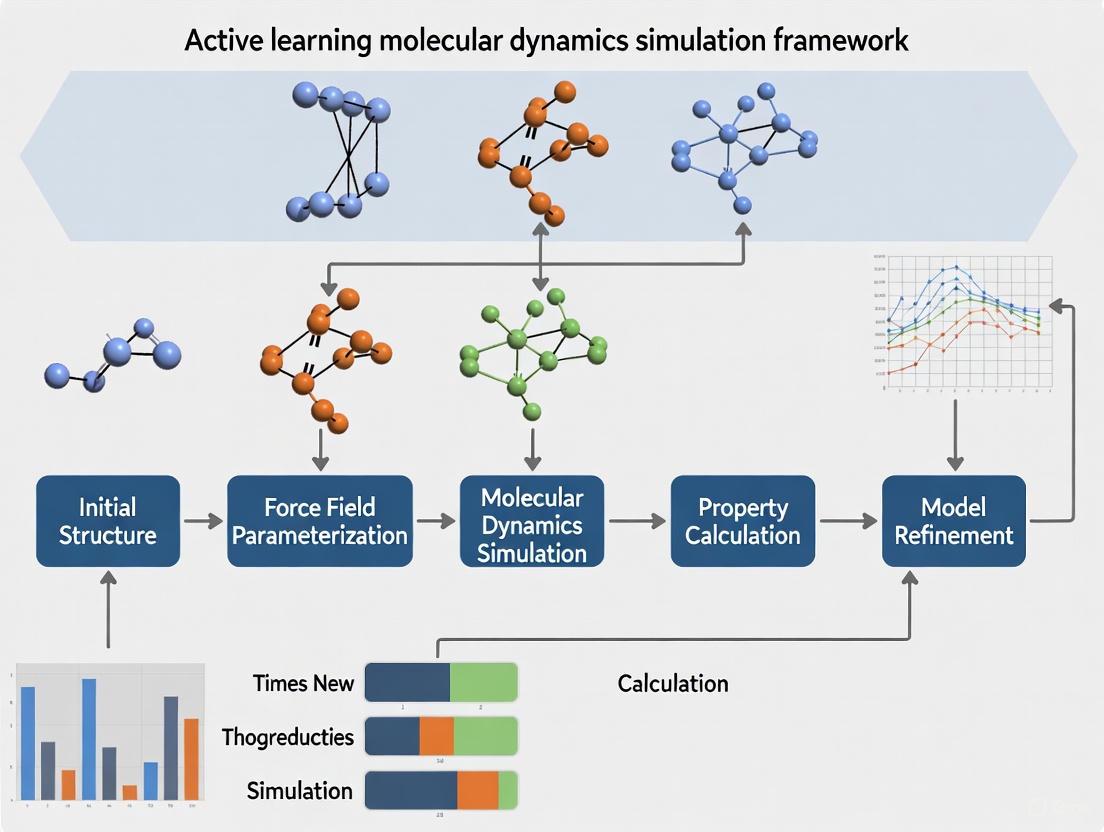
Active Learning Molecular Dynamics Framework
Core Framework Components
The active learning molecular dynamics framework comprises several interconnected components that work in concert to enable efficient exploration of chemical and conformational space. The foundational elements include molecular dynamics simulations for conformational sampling, machine learning models for prediction and guidance, and experimental validation to close the learning loop [1] [22].
Table 1: Core Components of Active Learning Molecular Dynamics Frameworks
| Component | Function | Implementation Examples |
|---|---|---|
| Receptor Ensemble Generation | Captures protein flexibility and multiple conformational states | ≈100-µs MD simulation of apo receptor; 20 snapshots for docking [1] |
| Target-Specific Scoring | Evaluates potential inhibitors based on structural features | Empirical score rewarding S1 pocket occlusion and reactive feature distances [1] |
| Active Learning Cycle | Intelligently selects compounds for subsequent evaluation | Iterative batch selection based on scoring function rankings [1] [22] |
| Molecular Dynamics Validation | Refines docking poses and eliminates false positives | 10-ns simulations of protein-ligand complexes; 100 ns per ligand [1] |
Quantitative Performance Advantages
Recent implementations of active learning frameworks have demonstrated significant improvements in efficiency and effectiveness compared to traditional virtual screening approaches. The quantitative advantages are substantial across multiple metrics relevant to drug discovery pipelines.
Table 2: Performance Comparison of Screening Approaches
| Metric | Traditional Docking Score | Active Learning with Target-Specific Score | Improvement Factor |
|---|---|---|---|
| Computational Screening | 2,755.2 compounds | 262.4 compounds | ~10.5x reduction |
| Simulation Time | 15,612.8 hours | 1,486.9 hours | ~10.5x reduction |
| Experimental Screening | Top 1,299.4 compounds | Top 5.6 compounds | ~232x reduction |
| Known Inhibitor Ranking | Correlation of 0.2 | Correlation of 1.0 | 5x improvement |
The performance advantages extend beyond simple efficiency metrics. In one implementation, the active learning approach reduced computational costs by approximately 29-fold while maintaining high accuracy in identifying true inhibitors [1]. This dramatic improvement stems from the framework's ability to focus resources on chemically relevant regions and avoid wasteful exploration of unproductive chemical space.
Application Notes: Case Studies
TMPRSS2 Inhibitor Discovery
A notable application of active learning molecular dynamics led to the identification of BMS-262084 as a potent inhibitor of TMPRSS2, with an experimental IC50 of 1.82 nM [1]. This discovery exemplifies the power of combining MD simulations with active learning for efficient navigation of chemical space.
Experimental Protocol:
- Receptor Ensemble Preparation: Generated a ≈100-µs MD simulation of TMPRSS2 and selected 20 snapshots representing conformational diversity [1]
- Initial Library Screening: Conducted molecular docking of 1% of the DrugBank library against the receptor ensemble
- Target-Specific Scoring: Implemented an empirical scoring function that rewarded occlusion of the S1 pocket and adjacent hydrophobic patch, with short distances for reactive and recognition states [1]
- Active Learning Cycles: Iteratively selected extension sets of compounds based on the target-specific score, with each set comprising 1% of the library
- Dynamic Validation: Performed 10-ns MD simulations of protein-ligand complexes for top-ranking candidates (totaling 100 ns per ligand) to eliminate false positives [1]
- Experimental Verification: Conducted cell-based assays confirming BMS-262084's efficacy in blocking entry of various SARS-CoV-2 variants and other coronaviruses [1]
The target-specific score was critical to the success of this approach, significantly outperforming conventional docking scores with a sensitivity of 0.5 compared to 0.38 [1]. When combined with MD-based validation, the sensitivity increased further to 0.88, demonstrating the value of incorporating protein flexibility and dynamic information [1].
Generative Active Learning for 3CLpro and TNKS2
A second case study employed a generative active learning protocol combining REINVENT (a generative molecular AI) with precise binding free energy ranking simulations using ESMACS [22]. This approach discovered new ligands for two different target proteins: 3CLpro and TNKS2.
Experimental Protocol:
- Generative Design: Used REINVENT to generate novel molecular structures based on initial training data [22]
- Binding Affinity Prediction: Employed ESMACS for absolute binding free energy calculations via molecular dynamics simulations [22]
- Active Learning Cycle: Selected batches of molecules for free energy assessment based on generative model predictions
- Batch Size Optimization: Varied batch sizes in each GAL cycle to determine optimal values for different scenarios [22]
- Chemical Space Analysis: Evaluated discovered ligands for chemical diversity and novelty compared to baseline compounds [22]
This implementation demonstrated the protocol's capability to discover higher-scoring molecules compared to baseline approaches, with the found ligands occupying distinct chemical spaces from known compounds [22]. The deployment on Frontier, the world's only exascale machine, enabled unprecedented sampling of chemical space through the combination of physics-based and AI methods [22].
Visualization and Workflow Diagrams
Active Learning Molecular Dynamics Workflow
Active Learning MD Screening Process
Coarse-Grained Active Learning Framework
CG to AA Active Learning Cycle
Research Reagent Solutions
Successful implementation of active learning molecular dynamics requires specialized computational tools and resources. The following table details essential research reagents and their functions in the framework.
Table 3: Essential Research Reagent Solutions for Active Learning MD
| Reagent/Tool | Function | Application Notes |
|---|---|---|
| Receptor Ensemble | Multiple protein conformations for docking | 20 snapshots from ≈100-µs MD simulation; critical for capturing binding-competent states [1] |
| Target-Specific Score | Empirical or learned scoring function | For TMPRSS2: rewards S1 pocket occlusion; for trypsin-domain proteins: random forest regressor with ∆SASA features [1] |
| Molecular Dynamics Engine | All-atom simulation capability | Enables 10-100 ns validation simulations; requires ≈818 µs total for 8180 ligands [1] |
| Active Learning Selector | Intelligent batch compound selection | Reduces experimental testing to <20 compounds; cuts computational costs by ~29-fold [1] |
| Coarse-Grained Neural Network | CGSchNet for accelerated sampling | Graph neural network using continuous filter convolutions; enables longer timescales [3] |
| All-Atom Oracle | High-accuracy reference calculations | OpenMM simulations for ground-truth forces; queried selectively via active learning [3] |
Implementation Protocols
Protocol 1: Structure-Based Active Learning Screening
This protocol details the implementation of a structure-based active learning framework for molecular discovery, optimized for targets with known structural information.
Step 1: Receptor Preparation and Ensemble Generation
- Conduct extensive MD simulations (≈100 µs) of the apo receptor to sample conformational diversity [1]
- Select 20 representative snapshots that capture distinct binding-competent states
- Validate ensemble diversity through RMSD clustering and binding site analysis
Step 2: Initial Library Docking and Scoring
- Dock a small initial set (1% of library) to all receptor conformations
- Apply target-specific scoring function (static h-score) to rank compounds
- For TMPRSS2-like targets: use empirical score based on S1 pocket occlusion and hydrophobic patch interactions [1]
- For general trypsin-domain proteins: implement learned score using random forest regressor trained on ∆SASA values and residue distances [1]
Step 3: Active Learning Cycle Implementation
- Select top-ranking compounds for MD validation (10-ns simulations per complex)
- Compute dynamic h-scores from MD trajectories to eliminate false positives
- Choose subsequent batch based on consensus ranking from multiple scoring approaches
- Continue iterations until convergence (typically 4-6 cycles) or identification of high-confidence hits
Step 4: Experimental Validation
- Synthesize or source top-ranked compounds for experimental testing
- Conduct biochemical assays to determine IC50 values
- Validate cellular efficacy in relevant disease models [1]
Protocol 2: Generative Active Learning with Coarse-Graining
This protocol implements a generative active learning approach combining AI-driven molecular design with coarse-grained molecular dynamics for enhanced efficiency.
Step 1: Initial Data Generation and Model Training
- Generate initial all-atom MD dataset for target system
- Train CGSchNet neural network potential via force matching:
- Use continuous filter convolutions based on inter-bead distances
- Minimize force matching loss: ℒℱℳ(θ) = (1/T)∑‖𝐅θ(𝐑) - 𝐅CG‖² [3]
- Ensure rotational and translational invariance in energy predictions
Step 2: Active Learning with Uncertainty Sampling
- Run CG MD simulations using trained neural network potential
- Calculate RMSD between simulation frames and training dataset
- Select frames with largest RMSD values (greatest conformational differences)
- Backmap selected frames to all-atom resolution using projection operators [3]
Step 3: Oracle Query and Dataset Expansion
- Query all-atom oracle (OpenMM) for selected configurations to obtain reference forces [3]
- Project all-atom forces back to CG space using force projection operator: 𝐅CG = ΞF𝐟AA [3]
- Append new data to training dataset with emphasis on coverage gaps
Step 4: Model Retraining and Validation
- Retrain CGSchNet on expanded dataset
- Validate using TICA (Time-lagged Independent Component Analysis) and free-energy metrics [3]
- Target >30% improvement in Wasserstein-1 metric in TICA space compared to baseline [3]
- Repeat active learning cycles until performance convergence
Discussion and Outlook
The integration of active learning with molecular dynamics simulations represents a paradigm shift in computational molecular discovery. By strategically guiding computational and experimental resources, these frameworks achieve unprecedented efficiency in navigating complex chemical and conformational spaces. The case studies presented demonstrate tangible successes, from the discovery of potent nanomolar inhibitors to the generation of novel chemical entities with desired binding properties.
Future developments in active learning molecular dynamics will likely focus on several key areas. Multiscale simulation methodologies will bridge wider temporal and spatial scales, while high-performance computing technologies like exascale computing will enable more comprehensive sampling [22] [23]. The integration of experimental and simulation data through automated platforms will create closed-loop discovery systems, and increased emphasis on environmental impact will drive the development of greener molecular solutions [23]. As these technologies mature, active learning molecular dynamics frameworks will become increasingly central to molecular design and optimization across pharmaceutical, materials, and chemical industries.
The protocols and application notes provided herein offer researchers practical guidance for implementing these powerful methodologies, with specific examples demonstrating their effectiveness in real-world discovery campaigns.
Implementing Active Learning MD: From Spectra Prediction to Drug Design
The development of machine-learned interatomic potentials (MLIPs) has become a cornerstone of modern atomistic simulation, enabling large-scale molecular dynamics (MD) with quantum-mechanical accuracy. A significant bottleneck in this process remains the manual generation and curation of high-quality training data. This challenge has spurred the creation of automated software frameworks that leverage active learning to efficiently explore potential-energy surfaces and construct robust MLIPs. Within the broader thesis on active learning molecular dynamics simulation frameworks, this application note provides a detailed examination of two key open-source frameworks, PALIRS and autoplex, and contextualizes them alongside established commercial modeling suites. We present structured quantitative data, detailed experimental protocols, and essential workflow visualizations to guide researchers and drug development professionals in implementing these powerful tools.
The autoplex Framework
autoplex ("automatic potential-landscape explorer") is an openly available software package designed to automate the exploration of potential-energy surfaces and the fitting of MLIPs [11] [24]. Its core innovation lies in automating iterative random structure searching (RSS) and model training, significantly reducing the human effort required to develop MLIPs from scratch. The framework is modular and interoperable with existing computational materials science infrastructures, notably building upon the atomate2 workflow system that underpins the Materials Project [11] [25]. A key application of autoplex is its integration with Gaussian Approximation Potentials (GAP), leveraging their data efficiency for tasks ranging from modeling elemental systems like silicon to complex binary systems such as titanium-oxygen [11] [24].
The PALIRS Framework
PALIRS (Python-based Active Learning Code for Infrared Spectroscopy) is an open-source active learning framework specifically designed for the efficient prediction of IR spectra using MLIPs [5]. It addresses the computational expense of ab-initio molecular dynamics (AIMD) for IR spectroscopy by training MLIPs on strategically selected data. The framework employs an active learning cycle to iteratively improve a neural network-based MLIP (e.g., MACE models), and separately trains a model for molecular dipole moment prediction, which is crucial for calculating IR spectra from MD trajectories [5].
Commercial Modeling Suites
Commercial software suites provide integrated, user-friendly environments for multiscale materials modeling. These platforms often combine various simulation engines, analysis tools, and workflow automation capabilities.
- MedeA (Materials Design, Inc.): An environment that integrates multiple simulation engines (e.g., VASP, LAMMPS, Gaussian) for property prediction and materials discovery. Its high-throughput modules, HT-Launchpad and HT-Descriptors, facilitate the generation of large, consistent datasets for screening and optimizing materials, creating input for machine learning procedures [26].
- Materials Studio (BIOVIA): A comprehensive modeling environment that includes quantum, atomistic, mesoscale, and statistical tools. Its integration with the Pipeline Pilot platform allows for the automation of routine calculations and the deployment of complex, multistep workflows as reusable "protocols," including for polymer informatics [26].
- CULGI: A software suite covering quantum mechanics to coarse-grained modeling and informatics. It features scripted workflows and a multiscale approach, enabling the building and simulation of complex systems, such as creating coarse-grained polymer structures and then reverse-mapping them to all-atom representations for further MD study [26].
Table 1: Key Features of Software Frameworks for Atomistic Modeling
| Framework | Primary Focus | Core Methodology | Key Automation Feature | Reported Output/Accuracy |
|---|---|---|---|---|
| autoplex [11] [24] | General-purpose MLIP development | Random Structure Searching (RSS) & iterative fitting | Automated workflow for exploration, data assembly, and fitting | Energy RMSE of ~0.01 eV/atom for Si allotropes [11] |
| PALIRS [5] | Infrared spectra prediction | Active learning for MLIP & dipole moment training | Iterative data selection based on uncertainty in forces | Accurate IR peak positions/amplitudes vs. AIMD/experiment [5] |
| MedeA [26] | Integrated multiscale materials engineering | High-throughput computation & workflow management | HT-Launchpad for automated high-throughput screening | Enables generation of descriptors for machine learning [26] |
| Materials Studio [26] | Integrated multiscale materials science | Multiscale simulation & informatics | Pipeline Pilot for protocol creation and workflow automation | Streamlines polymer property prediction and catalyst design [26] |
| CULGI [26] | Complex chemical systems, formulations | Multiscale modeling (QM to mesoscale) | Scripted workflows for cross-scale simulation | Calibrates coarse-grained models using COSMO-RS thermodynamics [26] |
Experimental Protocols and Workflows
Protocol for Automated MLIP Development with autoplex
The following methodology outlines the procedure for developing a robust MLIP using the autoplex framework, as demonstrated for the titanium-oxygen system [11] [24].
Initialization and System Definition:
- Define the chemical system (e.g., elemental, binary like Ti-O) and set the initial RSS parameters. This includes specifying the composition space to be explored.
- Configure the computational parameters for the underlying density-functional theory (DFT) calculations that will serve as the reference data source.
Iterative Exploration and Training Cycle:
- Step 1: Structure Generation. Generate a batch (e.g., 100) of random initial atomic structures within the defined chemical system.
- Step 2: MLIP Relaxation. Relax these generated structures using the current, best-available MLIP (initially, this may be a very simple model or non-existent, requiring the first iteration to use DFT).
- Step 3: DFT Single-Point Calculations. Perform single-point DFT energy and force calculations on the MLIP-relaxed structures. This step provides the quantum-mechanical reference data without the cost of full DFT molecular dynamics.
- Step 4: Dataset Expansion. Add the new structures and their DFT-calculated energies and forces to the training dataset.
- Step 5: MLIP Refitting. Retrain the MLIP (e.g., a GAP model) on the expanded training dataset to create an improved potential.
- Step 6: Error Evaluation. Evaluate the new model's accuracy on a set of known reference structures (e.g., crystalline polymorphs) by calculating the root mean square error (RMSE) of energies. The cycle (Steps 1-6) is repeated until the energy RMSE for key phases falls below a target threshold (e.g., 0.01 eV/atom) [11].
Validation and Production Simulation:
- Validate the final MLIP by comparing its predictions for properties (e.g., lattice parameters, relative phase energies) against pure DFT calculations or experimental data.
- Use the validated MLIP for large-scale or long-time MD simulations to investigate target phenomena.
Protocol for IR Spectra Prediction with PALIRS
This protocol details the four-step workflow for predicting accurate IR spectra of small organic molecules using the PALIRS framework [5].
Initial Data Preparation and MLIP Training:
- Step 1: Initial Dataset. For the target molecules, generate an initial set of molecular geometries by sampling along their normal vibrational modes. Compute reference energies and forces for these geometries using DFT.
- Step 2: Initial MLIP Training. Train an initial ensemble of MLIPs (e.g., MACE models) on this small dataset. An ensemble is used to estimate the uncertainty of force predictions.
Active Learning Cycle for MLIP Refinement:
- Step 3: ML-Driven MD (MLMD). Perform molecular dynamics simulations using the current MLIP at multiple temperatures (e.g., 300 K, 500 K, 700 K) to explore a broad configurational space.
- Step 4: Uncertainty-Based Acquisition. From the MLMD trajectories, select molecular configurations where the MLIP ensemble shows the highest uncertainty in its force predictions.
- Step 5: Oracle Query. Perform DFT calculations on the acquired structures to obtain accurate energies and forces.
- Step 6: Dataset Expansion and Retraining. Add these new data points to the training set and retrain the MLIP. Iterate Steps 3-6 until the model's performance on a validation set (e.g., harmonic frequencies) converges.
Dipole Moment Model Training and IR Spectra Calculation:
- Step 7: Dipole Model Training. Using the final, converged active learning dataset, train a separate ML model (e.g., a MACE model configured for dipole prediction) to predict the molecular dipole moment for any given atomic configuration.
- Step 8: Production MLMD for Spectra. Run a final, long MLMD production simulation using the refined MLIP (for energies and forces) and the dipole model.
- Step 9: IR Spectra Generation. Compute the IR spectrum by calculating the autocorrelation function of the dipole moment time series recorded during the production MLMD trajectory.
Key Reagents and Computational Materials
The following table details the essential software, tools, and computational "reagents" required to implement the protocols described for the autoplex and PALIRS frameworks.
Table 2: Essential Research Reagent Solutions for Active Learning MD
| Item Name | Type | Function in Protocol | Example/Note |
|---|---|---|---|
| Density Functional Theory (DFT) Code | Software Engine | Serves as the "oracle" for generating reference quantum-mechanical data (energies, forces) during training [11] [5]. | FHI-aims [5]; VASP is also commonly used. |
| MLIP Architecture | Core Model | Machine-learning model that learns the interatomic potential from DFT data. | Gaussian Approximation Potential (GAP) [11]; MACE [5]. |
| Active Learning Scheduler | Software Module | Manages the iterative workflow: launches searches/MD, queries oracle, and triggers retraining [11] [5]. | Built into autoplex and PALIRS. |
| Molecular Dynamics Engine | Software Engine | Propagates the dynamics of the atomic system using forces from the MLIP. | Can be an internal engine or link to external codes like LAMMPS. |
| Uncertainty Quantifier | Algorithmic Method | Identifies regions of configurational space where the MLIP is uncertain, guiding data acquisition [5]. | Ensemble of MACE models [5]; intrinsic variance in GAP [11]. |
| Structure Generator | Algorithmic Method | Creates diverse initial atomic configurations for exploration. | Random Structure Searching (RSS) in autoplex [11]. |
| Dipole Moment Predictor | Machine Learning Model | Predicts the electronic dipole moment of a configuration for IR intensity calculation [5]. | A separately trained MACE model in PALIRS [5]. |
Results and Performance Data
The performance of the autoplex and PALIRS frameworks is demonstrated through quantitative benchmarks on representative systems.
Table 3: Performance Benchmarks for the autoplex Framework on Material Systems [11] [24]
| Material System | Tested Structure/Phase | Key Performance Metric | Reported Result |
|---|---|---|---|
| Elemental Silicon (Si) | Diamond-type | Energy RMSE (eV/atom) | ~0.01 eV/atom after ~500 DFT single-points [11] |
| β-tin-type | Energy RMSE (eV/atom) | ~0.01 eV/atom after ~500 DFT single-points [11] | |
| oS24 allotrope | Energy RMSE (eV/atom) | ~0.01 eV/atom after a few thousand DFT single-points [11] | |
| Titanium Dioxide (TiO₂) | Anatase | Energy RMSE (eV/atom) | ~0.1 meV/atom (GAP-RSS on TiO₂ only) [24] |
| Brookite | Energy RMSE (eV/atom) | ~10 meV/atom (GAP-RSS on TiO₂ only) [24] | |
| Full Ti-O System | Rocksalt-type TiO | Energy RMSE (eV/atom) | Achieved target accuracy, requiring more iterations [11] |
Table 4: Performance Outcomes for the PALIRS Framework [5]
| Assessment Aspect | Metric | Outcome |
|---|---|---|
| Active Learning Efficacy | Model improvement on test set of harmonic frequencies | Mean Absolute Error (MAE) reduced through iterative active learning cycles [5]. |
| IR Spectra Accuracy | Comparison of peak positions and amplitudes | Agreement with both AIMD references and available experimental data [5]. |
| Computational Efficiency | Speedup vs. AIMD | MLIP-based MD simulations reported to be orders of magnitude faster than AIMD [5]. |
| Dataset Efficiency | Final dataset size for 24 organic molecules | ~16,067 structures after 40 active learning iterations (~600-800 structures/molecule) [5]. |
Infrared (IR) spectroscopy serves as a pivotal analytical tool across chemistry, biology, and materials science, providing real-time molecular insight into material structures and enabling the observation of reaction intermediates in situ. [5] However, interpreting experimental IR spectra is challenging due to peak shifts and intensity variations caused by molecular interactions and spectral congestion. [5] Traditional theoretical methods like density functional theory (DFT)-based ab-initio molecular dynamics (AIMD) provide higher-fidelity simulations that include anharmonic effects but are computationally prohibitive for large systems and high-throughput screening. [5]
The integration of machine learning (ML) with molecular dynamics (MD) offers a promising path to overcome these limitations. This case study explores the Python-based Active Learning Code for Infrared Spectroscopy (PALIRS) framework, which leverages an active learning-enhanced machine-learned interatomic potential (MLIP) to efficiently and accurately predict the IR spectra of small, catalytically relevant organic molecules. [5] By demonstrating accuracy comparable to AIMD at a fraction of the computational cost, PALIRS enables the exploration of larger catalytic systems and aids in identifying novel reaction pathways. [5]
The PALIRS framework implements a novel four-step approach designed to efficiently construct training datasets and predict IR spectra. [5] Its core innovation lies in using an active learning strategy to train a machine-learned interatomic potential (MLIP), which is then used for molecular dynamics simulations to calculate IR spectra. [5]
The following workflow diagram illustrates the key stages of the PALIRS computational process:
Core Components of the PALIRS Workflow
Step 1: Active Learning for MLIP Training: PALIRS initiates with an initial dataset of molecular geometries sampled along normal vibrational modes from DFT calculations. [5] An initial MLIP based on the MACE (Message Passing with Equivariant Representations) architecture is trained on this data. [5] This model is then refined through an active learning loop where MLMD simulations are run at different temperatures (300 K, 500 K, and 700 K) to explore configurational space. [5] Structures with the highest uncertainty in force predictions are selected to augment the training set, progressively improving the model's accuracy and generalizability. [5] After approximately 40 iterations, the final dataset comprises about 16,000 structures. [5]
Step 2: Dipole Moment Model Training: A separate ML model, also based on MACE, is specifically trained to predict molecular dipole moments, which are crucial for computing the IR absorption intensity. [5] This specialization ensures accurate prediction of both peak positions and amplitudes in the final spectrum. [5]
Step 3: Machine Learning-Assisted Molecular Dynamics (MLMD): The refined MLIP from Step 1 is used to run extensive MD simulations, generating trajectories that naturally include anharmonic effects. [5] These simulations are orders of magnitude faster than comparable AIMD. [5]
Step 4: IR Spectrum Calculation: Dipole moments are predicted for each structure along the MLMD trajectory using the model from Step 2. [5] The IR spectrum is then derived by computing the Fourier transform of the dipole moment autocorrelation function. [5]
Active Learning Methodology
The active learning cycle is the cornerstone of the PALIRS framework, ensuring computational efficiency and model robustness.
Active Learning Algorithm and Implementation
The active learning process strategically selects the most informative data points for DFT labeling, minimizing computational cost while maximizing model performance. [5] The detailed logical flow of this cycle is as follows:
PALIRS employs an ensemble of three MACE models to approximate prediction uncertainty, a key feature for the active learning acquisition function. [5] The acquisition strategy selects molecular configurations with the highest uncertainty in force predictions from MLMD runs conducted at multiple temperatures. [5] This multi-temperature approach balances exploration (high temperature) and exploitation (low temperature), ensuring comprehensive coverage of the relevant configurational space. [5] The iterative process continues until the MLIP's performance on a validation set of harmonic frequencies converges, typically after about 40 cycles. [5]
Performance and Validation
Quantitative Accuracy Assessment
The performance of PALIRS was rigorously validated against both AIMD benchmarks and experimental data for small organic molecules. [5] Key quantitative results demonstrate its effectiveness:
Table 1: Performance Metrics of PALIRS for IR Spectrum Prediction
| Metric | Performance | Validation Method | Significance |
|---|---|---|---|
| Computational Cost | "Fraction of the cost" of AIMD [5] | Comparative simulation | Enables high-throughput screening of larger systems [5] |
| Peak Position Accuracy | Agrees well with experimental data [5] | Experimental IR spectra | Reliable identification of molecular species [5] |
| Peak Amplitude Accuracy | Agrees well with experimental data [5] | Experimental IR spectra | Accurate prediction of band intensities [5] |
| Dataset Efficiency | Final dataset: 16,067 structures [5] | Active learning convergence | Minimizes expensive DFT calculations [5] |
| Training Trajectory | Initial MAE: ~40 cm⁻¹; Final MAE: ~8 cm⁻¹ [5] | Harmonic frequency MAE vs DFT | Demonstrates active learning efficacy [5] |
Convergence and Error Analysis
The active learning process significantly improves model accuracy. The learning curve shows a dramatic decrease in the mean absolute error (MAE) for harmonic frequencies compared to DFT references. [5] The initial MAE of approximately 40 cm⁻¹ is reduced to about 8 cm⁻¹ after active learning convergence. [5] This high level of accuracy is achieved with a final dataset of approximately 600-800 structures per molecule, demonstrating the data efficiency of the active learning paradigm. [5]
Experimental Protocol
This section provides a detailed, step-by-step protocol for predicting the IR spectrum of a catalytic molecule using the PALIRS framework.
System Setup and Initial Data Generation
- Molecule Selection: Identify the target small organic molecule(s) relevant to your catalytic system.
- Initial Structure Preparation: Obtain a reasonable 3D molecular structure. While not necessarily fully optimized, the structure should not have excessively high forces to ensure stable MD simulations. [6]
- Reference Engine Configuration:
- Software: Use the FHI-aims code for DFT calculations as implemented in PALIRS. [5]
- Settings: Employ consistent settings (functional, basis set, convergence criteria) used for generating the reference data. In a general active learning setup, other engines like ADF or DFTB can also be used if licensed. [6]
- Generate Initial Training Data:
- Perform normal mode analysis on the target molecule(s) using the reference DFT engine. [5]
- Sample molecular geometries by displacing atoms along the normal vibrational modes. [5]
- Run single-point DFT calculations on these displaced geometries to obtain reference energies, forces, and dipole moments. This creates the initial training set (e.g., ~2000 structures for 24 molecules). [5]
Active Learning for MLIP Training
- Model Architecture Selection: Choose an MLIP architecture. PALIRS uses an ensemble of three MACE models. [5]
- Configure Active Learning Parameters:
- Execute Active Learning Loop:
- Train MLIP: Train the ensemble model on the current training set.
- Run MLMD: Perform molecular dynamics simulations at different temperatures using the current MLIP.
- Query Data: Identify structures from the trajectories where the model exhibits the highest uncertainty in force prediction.
- Run Reference Calculations: Perform DFT calculations on the selected high-uncertainty structures to obtain accurate energies and forces.
- Augment Dataset: Add these new structures and their reference data to the training set.
- Check Convergence: Monitor the MAE of harmonic frequencies on a validation set. Repeat the loop until convergence is achieved. [5]
Dipole Moment Model Training
- Compile Dataset: Using the final structures from the active learning process, compile a dataset of molecular geometries and their corresponding DFT-calculated dipole moments. [5]
- Train Model: Train a separate MACE model specifically to predict dipole moment vectors. This model uses the geometries as input but is trained solely to predict the dipole moment, not energies or forces. [5]
Production Simulation and Spectrum Generation
- Run Production MLMD:
- Using the final, trained MLIP, run a long, well-equilibrated molecular dynamics simulation (e.g., >100 ps) of the target molecule at the desired temperature.
- Save the trajectory of atomic coordinates at regular intervals (e.g., every 1-5 fs).
- Predict Dipole Moments:
- For every saved snapshot (geometry) in the production trajectory, use the dedicated dipole moment model to predict the full dipole moment vector.
- Calculate IR Spectrum:
- Compute the time autocorrelation function of the total dipole moment vector from the trajectory.
- Apply Fourier transform to this autocorrelation function.
- The resulting power spectrum is the predicted IR spectrum. [5]
The Scientist's Toolkit: Essential Research Reagents and Computational Solutions
Table 2: Key Computational Tools and Resources for PALIRS Implementation
| Tool/Solution | Type | Function in Workflow |
|---|---|---|
| PALIRS Software [5] | Open-source package | Core framework implementing the active learning workflow and IR spectrum calculation. |
| MACE Model [5] | Machine Learning Interatomic Potential | Neural network architecture for predicting energies, forces, and dipole moments. |
| FHI-aims [5] | Density Functional Theory (DFT) Code | Reference electronic structure engine for generating accurate training data. |
| LUMI/CSC Supercomputers [27] | High-Performance Computing (HPC) Infrastructure | Provides the computational power required for DFT calculations and ML training. |
| Active Learning Algorithm [5] | Computational Method | Intelligently selects the most informative data points to minimize DFT costs. |
| Normal Mode Sampling [5] | Sampling Technique | Generates initial training data efficiently by exploring fundamental vibrations. |
The PALIRS framework demonstrates a significant advancement in the computational prediction of IR spectra by synergistically combining active learning, machine-learned interatomic potentials, and molecular dynamics. It successfully addresses the critical trade-off between computational cost and accuracy that has limited the application of high-fidelity simulations. By providing an efficient and automated path from molecular structure to accurate IR spectra, PALIRS opens new possibilities for high-throughput investigation of complex catalytic systems and reaction pathways, directly supporting the broader research objectives in active learning molecular dynamics simulation frameworks.
The drug discovery process traditionally resembles finding a needle in a haystack, characterized by extensive timelines, high costs, and significant attrition rates [1] [28]. The integration of artificial intelligence (AI) is fundamentally reshaping this paradigm, compressing discovery timelines that traditionally spanned years into months [29] [30]. Among the most promising advancements is the combination of generative AI for molecular design with active learning (AL) frameworks for guided exploration and validation [31] [28]. This synergy is particularly powerful when integrated with physics-based molecular dynamics (MD) simulations, which provide atomic-level insights into target engagement and binding stability [1] [31].
This case study examines the application of an integrated generative AI and active learning framework for de novo drug design. We present specific protocols and quantitative results from recent successful campaigns, including the identification of a broad coronavirus inhibitor and the generation of novel kinase binders. The content is structured to provide researchers with actionable methodologies, supported by data tables, workflow diagrams, and a detailed list of research reagents.
Integrated Workflow: Generative AI and Active Learning
The core of the modern de novo design pipeline involves a closed-loop system where a generative model proposes candidate molecules, and an active learning agent iteratively selects the most informative candidates for costly evaluation (e.g., simulation or experimentation), using the results to refine the model [31]. This feedback cycle efficiently navigates the vast chemical space toward molecules with desired properties.
Workflow Diagram
The following diagram illustrates the integrated generative AI and active learning framework, highlighting the iterative feedback loop that connects molecular generation, evaluation, and model refinement.
Case Study 1: Identifying a Broad Coronavirus Inhibitor
A 2025 study successfully identified a potent TMPRSS2 inhibitor by combining molecular dynamics (MD) simulations with an active learning framework, dramatically reducing the number of candidates requiring experimental testing [1].
Key Quantitative Outcomes
The following table summarizes the efficiency gains and key results from the TMPRSS2 inhibitor identification campaign.
| Metric | Docking Score Only | MD + Active Learning with Target-Specific Score | Efficiency Gain |
|---|---|---|---|
| Computational Screening | 2,755.2 compounds | 262.4 compounds | ~10.5x reduction |
| Simulation Time | 15,612.8 hours | 1,486.9 hours | ~10.5x faster |
| Experimental Screening | Top ~1,300 compounds | Top ~5-6 compounds | ~200x reduction |
| Identified Inhibitor | N/A | BMS-262084 (IC₅₀ = 1.82 nM) | Successful hit |
| Experimental Validation | N/A | Blocked entry of various SARS-CoV-2 variants and other coronaviruses in cell assays | Clinically relevant |
Detailed Experimental Protocol
Objective: To identify a potent, broad-spectrum TMPRSS2 inhibitor from large compound libraries with minimal experimental testing.
Step 1: Generate a Receptor Ensemble
- Protocol: Run an extensive (~100 µs) molecular dynamics (MD) simulation of the apo TMPRSS2 protein. From this trajectory, extract 20-30 structurally diverse snapshots to create a "receptor ensemble" that accounts for protein flexibility and multiple conformational states [1].
- Rationale: Docking to a single static structure may miss viable binding poses; an ensemble increases the likelihood of docking to binding-competent conformations [1].
Step 2: Initial Docking and Target-Specific Scoring
- Protocol: Dock the entire compound library (e.g., DrugBank, NCATS in-house library) against every structure in the receptor ensemble. Instead of relying on generic docking scores, calculate a target-specific "h-score" for each pose. This empirical score rewards:
- Occlusion of the S1 pocket and adjacent hydrophobic patch.
- Short distances between key ligand functional groups and catalytic residues (e.g., His296, Asp345) [1].
- Rationale: The target-specific score more accurately reflects the structural determinants of serine protease inhibition than standard docking functions [1].
Step 3: Active Learning Cycle
- Protocol:
- Initial Batch: Select the top 1% of candidates ranked by the static h-score.
- Iterative Extension:
- Experimentally test (or run more expensive MD simulations on) the selected batch.
- Use the results to update the active learning model.
- The model selects the next most informative batch of candidates (e.g., those with high prediction uncertainty or high predicted score) from the remaining library.
- Stopping Criterion: Cycle continues until all known inhibitors are ranked highly or a performance threshold is met [1].
- Rationale: Active learning focuses computational and experimental resources on the most valuable data points, drastically reducing the number of compounds that need evaluation [1] [32].
Step 4: Experimental Validation
- Protocol: Synthesize or procure the top-ranked compounds from the final AL cycle. Validate efficacy through:
- In vitro enzymatic assays (e.g., TMPRSS2 inhibition IC₅₀ measurement).
- Cell-based assays (e.g., viral entry inhibition in Calu-3 human lung cells across multiple SARS-CoV-2 variants) [1].
Case Study 2: Generating Novel Kinase Inhibitors with a VAE-Active Learning Framework
Another 2025 study demonstrated a generative AI workflow featuring a Variational Autoencoder (VAE) with two nested active learning cycles to design novel, synthesizable inhibitors for CDK2 and KRAS [31].
Key Quantitative Outcomes
The table below summarizes the experimental results for the novel CDK2 inhibitors generated and synthesized via the VAE-AL workflow.
| Metric | Result for CDK2 | Result for KRAS |
|---|---|---|
| Generated Molecules Meeting Criteria | Diverse, drug-like molecules with excellent docking scores and synthetic accessibility | Diverse, drug-like molecules with excellent docking scores |
| Molecules Selected for Synthesis | 10 molecules selected | N/A (In silico validation) |
| Successful Syntheses | 9 molecules | N/A |
| Experimentally Active Molecules | 8 out of 9 synthesized molecules | N/A |
| Potency of Best Hit | 1 molecule with nanomolar potency | 4 molecules with potential activity identified in silico |
Detailed Experimental Protocol
Objective: To generate novel, drug-like, and synthesizable small-molecule inhibitors for specific protein targets (CDK2 and KRAS) with high predicted affinity.
Step 1: Initial VAE Training
- Protocol:
- Data Representation: Represent training molecules as SMILES strings, which are tokenized and converted into one-hot encoding vectors.
- Two-Stage Training: First, pre-train the VAE on a large, general molecular dataset (e.g., ZINC). Then, fine-tune the VAE on a target-specific training set to bias the model towards relevant chemical space [31].
Step 2: Nested Active Learning Cycles The workflow employs two nested cycles that use different oracles to iteratively refine the generated molecules [31].
Inner AL Cycle (Chemical Space Refinement)
- Protocol:
- Generation: The fine-tuned VAE generates a large set of novel molecules.
- Cheminformatic Evaluation: Generated molecules are evaluated by a property oracle that assesses:
- Drug-likeness (e.g., Lipinski's Rule of Five).
- Synthetic Accessibility (SA) score.
- Dissimilarity from the initial training set (to ensure novelty).
- Fine-tuning: Molecules passing these filters are added to a "temporal-specific set," which is used to further fine-tune the VAE, pushing it to generate molecules with these desirable properties [31].
- Rationale: This inner cycle ensures the generative model focuses on a chemically feasible, novel, and drug-like region of chemical space before committing to more expensive affinity calculations.
Outer AL Cycle (Affinity-Driven Refinement)
- Protocol:
- Docking: After several inner cycles, molecules accumulated in the temporal set are evaluated by an affinity oracle (e.g., molecular docking against the target protein).
- Selection: Molecules meeting a docking score threshold are transferred to a "permanent-specific set."
- Fine-tuning: The VAE is fine-tuned on this permanent set, biasing future generation toward high-affinity candidates [31].
- Rationale: This cycle directly optimizes for the primary objective—target binding—using physics-based scoring, which is more reliable than data-driven predictors in low-data regimes [31].
Step 3: Candidate Selection and Experimental Validation
- Protocol: The final permanent-specific set undergoes rigorous filtration:
- Advanced Simulation: Use advanced MD simulations like Protein Energy Landscape Exploration (PELE) and Absolute Binding Free Energy (ABFE) calculations for an in-depth evaluation of binding interactions and stability [31].
- Synthesis and Assaying: Select top candidates for synthesis and validate their activity through in vitro biochemical and cell-based assays [31].
The Scientist's Toolkit: Research Reagent Solutions
The following table catalogues key computational and experimental reagents essential for implementing the described frameworks.
| Reagent / Tool | Type | Function in Workflow |
|---|---|---|
| Receptor Ensemble | Computational Model | A collection of protein structures from MD simulations used for docking to account for flexibility and avoid false negatives [1]. |
| Target-Specific Score (h-score) | Computational Metric | An empirical or learned scoring function tailored to a specific protein's active site, improving hit identification accuracy over generic scores [1]. |
| Variational Autoencoder (VAE) | Generative AI Model | A deep learning architecture that learns a continuous latent representation of molecules, enabling generation of novel molecular structures [31] [33]. |
| Molecular Dynamics (MD) Simulator | Simulation Software | Software that simulates physical movements of atoms and molecules over time, used for generating receptor ensembles and refining poses [1] [3]. |
| Docking Software | Computational Tool | Software that predicts the preferred orientation and pose of a small molecule when bound to a target protein [1] [31]. |
| PELE (Protein Energy Landscape Exploration) | Advanced Simulation Algorithm | A Monte Carlo-based algorithm used for rapid exploration of protein-ligand binding and unbinding pathways, aiding in candidate selection [31]. |
| Yeast Surface Display | Experimental Screening Platform | A high-throughput experimental method for screening thousands of designed protein binders (e.g., antibodies, VHHs) for affinity and specificity [34]. |
| OrthoRep | Experimental Platform | A yeast-based system for rapid in vivo mutagenesis and selection, used for affinity maturation of initially designed binders [34]. |
CGSchNet is a machine-learned, coarse-grained (CG) molecular dynamics model that leverages graph neural networks (GNNs) to simulate protein dynamics with a computational efficiency several orders of magnitude greater than all-atom molecular dynamics (MD) [35]. Developed using a bottom-up force-matching approach, it is trained on diverse datasets of all-atom protein simulations to learn effective physical interactions between CG degrees of freedom [35] [36]. Its key innovation is chemical transferability—the ability to perform extrapolative molecular dynamics on novel protein sequences not present in the training data [35]. When integrated into an Active Learning Molecular Dynamics (ALMD) framework, CGSchNet acts as a fast, surrogate propagator. An active learning loop corrects its forces when it encounters under-sampled conformations, creating a computationally efficient and self-correcting simulation system that is a cornerstone of modern computational biophysics [37] [3].
Application Notes: Key Use Cases and Performance
CGSchNet enables the investigation of complex biomolecular processes that are computationally prohibitive for all-atom simulations. The following table summarizes its core applications and documented performance.
Table 1: Key Applications and Performance of CGSchNet
| Application Domain | Key Functionality | Reported Performance & Quantitative Insights |
|---|---|---|
| Protein Folding Landscape Exploration | Predicts metastable states of folded, unfolded, and intermediate structures; simulates folding/unfolding transitions [35]. | Successfully folded small proteins (e.g., Chignolin, TRPcage, Villin) from extended states; reproduces free energy surfaces comparable to all-atom MD [35]. |
| Intrinsically Disordered Proteins (IDPs) | Models fluctuations and conformational dynamics of disordered protein regions [35]. | Accurately captures the conformational landscape of disordered peptides, matching atomistic reference data [35]. |
| Free Energy Calculations | Estimates relative folding free energies of protein mutants [35]. | Capable of predicting changes in free energy upon mutation, useful for protein engineering studies [35]. |
| Active Learning-Driven Correction | RMSD-based frame selection triggers all-atom simulation to correct CG model in under-sampled regions [37] [3]. | Achieved a 33.05% improvement in the Wasserstein-1 metric in TICA space for Chignolin, indicating superior reproduction of the reference distribution [3]. |
| Standardized Benchmarking | Integrated with Weighted Ensemble (WE) sampling for rare-event simulation and quantitative benchmarking [37]. | Fully trained models show close overlap with all-atom ground truth; under-trained models exhibit instability (e.g., implosion/explosion) [37]. |
Detailed Experimental Protocols
Protocol 1: Standard Simulation of a Protein's Conformational Landscape
This protocol details how to use a pre-trained CGSchNet model to simulate the free energy landscape of a protein, such as the fast-folding protein Chignolin.
Table 2: Key Research Reagents and Computational Solutions
| Item | Function/Description |
|---|---|
| Pre-trained CGSchNet Model | A neural network that takes CG coordinates as input and outputs the system's potential energy and forces [37] [3]. |
| CG Protein Structure File | Input file containing the initial coordinates of the protein's Cα beads. |
| Langevin Integrator | A stochastic differential equation solver that maintains a constant temperature during simulation by incorporating friction and noise terms [35]. |
| Parallel Tempering (PT) Setup | Enhanced sampling technique that runs multiple replicas of the system at different temperatures, allowing escape from local energy minima [35]. |
Procedure:
- System Initialization: Obtain the initial coordinates for the protein's Cα beads. For folding studies, start from an extended conformation or a known native structure.
- Simulation Engine: Configure the molecular dynamics engine to use the CGSchNet potential,
U_θ(R) = CGSchNet(R), where R represents the coordinates of the Cα beads [3]. Forces are calculated asF_θ(R) = -∇_R U_θ(R). - Sampling Configuration:
- For constant-temperature dynamics, use a Langevin integrator at 300 K to generate a long trajectory [35].
- For a converged equilibrium distribution, employ Parallel Tempering (PT). Typically, 16-32 replicas spanning a temperature range of 300-500 K are used to ensure efficient sampling of folding/unfolding events [35].
- Trajectory Analysis: Analyze the output trajectories using collective variables.
- Calculate the Fraction of Native Contacts (Q), which measures the similarity to the native folded state (Q=1 is fully folded, Q=0 is unfolded).
- Calculate the Cα Root-Mean-Square Deviation (Cα RMSD) from the native structure.
- Construct a 2D free energy surface (FES) as a function of Q and Cα RMSD using the formula:
ΔG(Q, RMSD) = -k_B T ln P(Q, RMSD), wherePis the probability distribution [35].
Protocol 2: Active Learning for Model Correction and Refinement
This protocol describes the iterative active learning loop used to improve CGSchNet when it encounters poorly sampled conformations.
Procedure:
- Initial Training: Train an initial CGSchNet model on an existing dataset of all-atom simulation data that has been projected into CG space [3].
- CG Simulation and Frame Selection: Run a CG molecular dynamics simulation using the trained model. From the resulting trajectory, select frames with the highest Root-Mean-Square Deviation (RMSD) compared to the existing training set. These high-RMSD frames represent the most under-sampled conformations [3].
- Backmapping and Oracle Query: Backmap the selected CG frames to all-atom representations. Use these all-atom structures as initial seeds to run short, targeted all-atom simulations with an oracle (e.g., OpenMM with a classical force field) [3].
- Projection and Dataset Augmentation: Project the new all-atom simulation data back to the CG representation, including coordinates and the corresponding mapped CG forces,
F_CG[3]. - Model Retraining: Retrain the CGSchNet model on the augmented dataset (original data + new active learning data). The core loss function minimized during training is the Force Matching loss [3]:
L_FM(θ) = (1/T) * Σ || F_θ(R) - F_CG ||² - Iteration: Repeat steps 2-5 until the model's performance converges, as measured by benchmarks like the Wasserstein-1 distance in a reduced dimensional space [3].
Workflow Visualization
The following diagram illustrates the integrated active learning framework for machine-learned molecular dynamics, combining the standard simulation and active learning protocols.
Active Learning Workflow for CGSchNet
The Scientist's Toolkit
Table 3: Essential Research Reagents and Computational Tools
| Category / Item | Specific Examples / Functions |
|---|---|
| Core Modeling & Simulation | |
| CGSchNet Software | Graph neural network architecture for learning CG force fields [36] [3]. |
| All-Atom MD Oracle (Quantum Chemistry) | OpenMM; provides reference forces and energies for training and active learning [3]. |
| Data Preparation & Mapping | |
| Mapping Operator (Ξ) | Linear projection R = Ξr that maps all-atom coordinates (r) to CG coordinates (R) [36] [3]. |
| Force Projection Operator (Ξ_F) | Projects all-atom forces to CG space: F_CG = Ξ_F f_AA [3]. |
| Sampling & Enhanced Dynamics | |
| Parallel Tempering (PT) | Enhanced sampling method for converging equilibrium distributions [35]. |
| Weighted Ensemble (WE) Sampling | WESTPA toolkit; rare-event sampling for benchmarking [37]. |
| Analysis & Validation | |
| Dimensionality Reduction | Time-lagged Independent Component Analysis (TICA) for constructing collective variables and progress coordinates [37]. |
| Benchmarking Metrics | Wasserstein-1 (W1) distance, Kullback-Leibler (KL) divergence, kernel density overlap [37]. |
| Structural Metrics | Fraction of Native Contacts (Q), Cα Root-Mean-Square Deviation/Flucutation (RMSD/RMSF), Radius of Gyration (Rg) [35] [37]. |
The discovery and development of novel materials have traditionally been slow, resource-intensive processes, often relying on sequential experimentation and researcher intuition. High-throughput materials exploration has emerged as a transformative paradigm, dramatically accelerating this cycle by integrating computational screening, automated experimentation, and data-driven informatics. This approach enables the rapid assessment of thousands to millions of material candidates, efficiently narrowing the experimental focus to the most promising compositions and synthesis routes. Within this framework, active learning molecular dynamics simulations provide a powerful foundation, iteratively guiding experimental design by predicting material properties and stability from atomic-scale interactions.
The transition "from silicon to complex binary oxides" represents an evolution from relatively simple, well-understood systems to multifunctional materials with enhanced capabilities but greater compositional complexity. This article details specific application notes and experimental protocols that operationalize this high-throughput discovery pipeline, providing researchers with implementable methodologies for next-generation materials development.
Application Notes: Integrated Computational-Experimental Workflows
Application Note AN-001: Deep Learning for Thermodynamic Property Prediction of Binary Composite Oxides
Objective: To accurately estimate the standard enthalpy of formation (ΔHf) for binary composite oxides (BCOs) using a novel deep learning architecture, bypassing traditional laborious calorimetric measurements.
Background: Predicting the stability and synthesizability of materials requires precise knowledge of thermodynamic properties. For BCOs, traditional experimental determination of ΔHf is a significant bottleneck in discovery pipelines.
Implementation: A hybrid deep learning model termed MHA-TCN-HO-SE (Multi-Head Attention-Temporal Convolutional Network-Hebbian Optimization-Standard Enthalpy) was implemented [38]. The model was trained on a comprehensive dataset compiled from literature, covering the standard enthalpy for 209 different BCOs formed from 33 simple oxides at 298 K [38].
- Data Curation: The dataset was constructed from peer-reviewed literature, ensuring a wide coverage of cationic combinations and crystal structures prevalent in BCOs.
- Model Architecture:
- Multi-Head Attention (MHA): Captures complex, non-local dependencies between input features (e.g., ionic radii, electronegativity, oxidation states).
- Temporal Convolutional Network (TCN): Models short- and long-range dependencies within the sequential data representation of material compositions.
- Hebbian Optimization (HO): Enhances feature learning and model convergence by applying neurobiological learning principles.
Key Performance Metrics: The model's performance was quantitatively evaluated against traditional methods and other machine learning models, as summarized in Table 1.
Table 1: Performance Comparison of Models for Standard Enthalpy Prediction [38]
| Model / Method | RMSE (KJ·mol⁻¹) | MAPE (%) | R² |
|---|---|---|---|
| MHA-TCN-HO-SE (Proposed) | 12.56 | 9.21 | 0.93 |
| TXL-GNN | 13.80 | 10.00 | 0.91 |
| NAS-LSTM | 14.50 | 10.80 | 0.89 |
| AGCN | 15.20 | 11.50 | 0.87 |
Insight for Researchers: The MHA-TCN-HO-SE model demonstrates strong generalization and stability across different training data proportions, making it suitable for predicting properties of novel BCO compositions outside the initial training set. Its superior performance provides a reliable in-silico tool for prioritizing synthesis targets.
Application Note AN-002: Discovery of Broad-Spectrum Coronavirus Inhibitors via Active Learning
Objective: To minimize the number of candidate compounds requiring experimental validation by combining molecular dynamics (MD) simulations with an active learning loop for virtual drug screening.
Background: Conventional virtual screening often struggles with the balance between computational cost and experimental correlation. This protocol addresses this by drastically reducing the number of candidates needing experimental testing to less than 20 [39].
Implementation:
- Initial MD Ensemble Generation: Extensive MD simulations were performed to generate a diverse ensemble of receptor conformations, capturing protein flexibility.
- Target-Specific Scoring: A custom scoring function was developed to evaluate the potential of compounds for inhibiting the target (e.g., TMPRSS2 protease).
- Active Learning Cycle:
- An initial batch of candidates was selected from a large virtual library using the scoring function.
- The top candidates from this batch were advanced to experimental testing.
- The experimental results (e.g., IC50 values) were fed back into the model to refine the scoring function and candidate selection for the next cycle.
- This iterative process continued until high-potency inhibitors were identified.
Outcome: This framework led to the discovery of BMS-262084, a potent inhibitor of TMPRSS2 with a half-maximal inhibitory concentration (IC50) of 1.82 nM [39]. Cell-based assays confirmed its efficacy against multiple SARS-CoV-2 variants and other coronaviruses.
Insight for Researchers: The active learning approach reduced computational costs by approximately 29-fold compared to a brute-force screening strategy [39]. This demonstrates the profound efficiency gains achievable when simulation is tightly coupled with experimental feedback, a principle directly applicable to materials discovery.
Application Note AN-003: Electronic Structure Similarity Screening for Bimetallic Catalysts
Objective: To identify bimetallic alloy catalysts that can replace or reduce the use of scarce palladium (Pd) in hydrogen peroxide (H2O2) synthesis.
Background: The electronic Density of States (DOS) is a key determinant of catalytic properties. Materials with similar electronic structures often exhibit similar catalytic behaviors [40].
Implementation:
- High-Throughput Computational Screening: Using Density Functional Theory (DFT), 4350 bimetallic alloy structures derived from 30 transition metals were screened for thermodynamic stability (formation energy, ΔEf < 0.1 eV) [40].
- Descriptor Calculation: The full DOS pattern (including d- and sp-states) of the closest-packed surface of each of the 249 thermodynamically stable alloys was calculated. The similarity to the DOS of the Pd(111) surface was quantified using a ΔDOS metric [40]:
- Experimental Validation: The top eight candidate alloys with the lowest ΔDOS values were synthesized and tested for H2O2 direct synthesis.
Outcome: Four of the eight candidates exhibited catalytic performance comparable to Pd. Notably, the Pd-free catalyst Ni61Pt39 outperformed Pd, showing a 9.5-fold enhancement in cost-normalized productivity [40].
Insight for Researchers: Using the full DOS pattern as a descriptor successfully captured reactivity trends that simpler metrics (e.g., d-band center alone) might miss, as evidenced by the critical role of sp-states in O2 adsorption [40]. This underscores the value of rich electronic structure data for predictive screening.
Experimental Protocols
Protocol P-001: High-Throughput Rapid Experimental Alloy Development (HT-READ)
Purpose: To provide a closed-loop, high-throughput methodology for the fabrication, testing, and analysis of alloy libraries, integrating computational guidance with automated experimentation [41].
Materials and Equipment:
- Computational Resources: CALPHAD software, Machine Learning models.
- Fabrication: Automated synthesis platform (e.g., Chemspeed Swing XL for solution-based synthesis, arc melter or sputtering system for solid alloys).
- Characterization: High-throughput X-ray Diffractometer (XRD), automated SEM/EDS, robotic mechanical testing systems.
- Data Management: A centralized database with unique sample identifiers.
Procedure:
- Computational Screening: Use CALPHAD and/or ML models to identify promising alloy compositions based on target properties (e.g., phase stability, modulus).
- Library Design & Fabrication:
- Design sample libraries in a geometry amenable to multiple tests (e.g., composition spread thin films or an array of small-scale buttons).
- Execute synthesis using an automated platform to ensure reproducibility and precise parameter control.
- High-Throughput Characterization:
- Perform rapid, automated structural characterization (e.g., XRD mapping) on all library members.
- Execute parallel property measurements (e.g., nanoindentation for hardness, electrical resistivity mapping).
- Data Analysis and AI-Driven Insight:
- Automatically process characterization data to label phases and extract properties.
- Feed all data into an AI/ML agent to identify composition-structure-property relationships.
- Iteration: Use the newly generated experimental data to refine the computational models and design the next iteration of the sample library.
Visual Workflow:
Protocol P-002: Kernel Learning-Assisted Synthesis of Ternary Spinel Oxides
Purpose: To optimize the synthesis parameters for single-phase mixed metal oxides (MMOs) using an interpretable kernel learning model trained on a sparse, high-throughput dataset [42].
Materials and Equipment:
- Precursors: Metal salts (e.g., Nitrates of Fe, Zn, Co), precipitating agent (e.g., K2CO3 solution).
- Synthesis Platform: Automated robotic synthesizer (e.g., Chemspeed Swing XL).
- Characterization: High-throughput X-ray Diffractometer (XRD).
Procedure:
- High-Throughput Experimentation (HTE):
- Define the experimental parameter space: precursor concentrations, reagent amounts, addition rate, and addition order (normal vs. reverse).
- Use the automated platform to synthesize a library of samples (~70 samples) via co-precipulation, systematically varying parameters.
- Phase Labeling:
- Characterize all samples using XRD.
- Label each sample as "single-phase" (dominant spinel phase) or "multi-phase" (presence of secondary oxide phases).
- Model Training and Interpretation:
- Train a kernel classification model on the dataset, using the five synthesis parameters as features and the phase label as the output.
- Perform global SHAP (SHapley Additive exPlanations) analysis to quantify the contribution of each synthesis parameter to the achievement of a single-phase product.
- Model-Guided Exploration:
- Use the trained model to predict the outcome of ~43,200 in-silico candidate experiments.
- Prioritize new experiments using an uncertainty sampling policy, focusing on the parameter space where the model is most confident about single-phase formation.
Key Findings: Global SHAP analysis revealed that the amount of reagents was a critically important feature for single-phase synthesizability, providing insights that align with crystal growth theories but may have been non-intuitive a priori [42].
Visual Workflow:
The Scientist's Toolkit: Essential Research Reagents & Materials
Table 2: Key Reagents and Materials for High-Throughput Materials Exploration
| Item | Function / Application | Example / Note |
|---|---|---|
| Chemspeed Swing XL | Automated robotic synthesis platform for precise control of synthesis parameters and high reproducibility [42]. | Used for co-precipitation of ternary spinels. |
| Transition Metal Precursors | Source of metallic elements for alloy and oxide formation. | Nitrates, chlorides, or acetylacetonates for oxides; pure metal pieces for alloy arc-melting. |
| K2CO3 Solution | Common precipitating agent for the synthesis of metal oxide powders. | Concentration is a key controlled parameter [42]. |
| CALPHAD Software | Computational tool for predicting phase stability and phase diagrams in alloy systems. | Used for initial thermodynamic screening in HT-READ [41]. |
| Density Functional Theory (DFT) | First-principles computational method for calculating electronic structure and energy. | Used for calculating formation energies and DOS patterns for screening [40]. |
| SHAP Analysis | Interpretable ML method to explain the output of any machine learning model. | Critical for understanding which synthesis parameters drive single-phase formation [42]. |
The integration of high-throughput computational screening, automated experimental platforms, and active learning frameworks represents a paradigm shift in materials science. The protocols outlined here—from predicting thermodynamic properties with deep learning to optimizing synthesis with interpretable kernel models—provide a concrete roadmap for accelerating the discovery of complex materials like binary oxides and multi-component alloys. By closing the loop between simulation and experiment, researchers can efficiently navigate vast compositional and processing spaces, dramatically reducing the time and cost required to bring new materials from concept to application. The future of this field lies in the continued development of multiscale simulation methodologies, the integration of high-performance computing, and the creation of standardized, shareable data infrastructures.
Optimizing Your AL-MD Workflow: Key Parameters and Common Pitfalls
In modern computational chemistry and drug development, Active Learning Molecular Dynamics (AL-MD) has emerged as a powerful framework for accelerating molecular simulations and improving the accuracy of interatomic potentials. A cornerstone of this iterative framework is the establishment of robust success criteria, primarily defined by energy and force error thresholds. These thresholds determine when the machine learning (ML) model requires augmentation with new quantum mechanical data, thereby balancing computational efficiency with predictive accuracy. Setting these criteria appropriately is crucial for generating reliable, generalizable potentials that can capture complex biomolecular processes relevant to drug discovery.
The core challenge in AL-MD lies in the inherent trade-off between computational cost and model fidelity. Without well-defined error thresholds, the active learning process can either fail to capture chemically relevant regions of configuration space or become computationally prohibitive due to excessive quantum calculations. This protocol details the theoretical foundation, quantitative benchmarks, and practical methodologies for establishing these critical energy and force error thresholds within an active learning molecular dynamics simulation framework, providing researchers with a standardized approach for implementing robust and efficient simulation campaigns.
Theoretical Foundation and Key Concepts
The Role of Uncertainty Quantification in Active Learning
Active learning relies fundamentally on quantifying the uncertainty of a machine-learned interatomic potential. In this paradigm, an ensemble of neural network potentials is typically trained on a set of quantum mechanical data. The disagreement in predictions (e.g., energies or forces) across the ensemble members serves as a proxy for the model's uncertainty when it encounters a new atomic configuration [14]. This ensemble disagreement, often measured by the standard deviation of predicted energies or forces normalized by the square root of the number of atoms (ρ), is the primary metric against which thresholds are applied [14]. When this uncertainty metric exceeds a predefined threshold, it signals that the current configuration is outside the model's reliable knowledge domain, triggering an expensive ab initio calculation to augment the training set and improve the model.
Energy and Force Error Metrics
The accuracy of an ML potential is primarily judged on its ability to reproduce the potential energies and atomic forces derived from high-fidelity quantum mechanics (e.g., Density Functional Theory). The error metrics for these properties are defined as:
- Force Error (eV/Å): The error in the force component on an individual atom. This is often the primary criterion for data selection due to its vector nature and higher sensitivity to local atomic environments compared to total energy [43].
- Energy Error (meV/atom): The error in the total potential energy of a configuration, normalized per atom. This ensures size-extensivity and allows for comparison across systems of different sizes.
These errors can be reported as Mean Absolute Error (MAE) or Root Mean Square Error (RMSE) over a validation set. However, within the active learning loop, it is the predicted uncertainty (from the ensemble) for a single new configuration that is compared to the threshold to decide on querying the oracle.
Establishing Quantitative Error Thresholds
Determining the specific numerical values for error thresholds is system-dependent, but general guidelines and practical values have emerged from the literature. The following table summarizes key quantitative error thresholds and their functional roles within the AL-MD framework.
Table 1: Key Energy and Force Error Thresholds in Active Learning MD
| Threshold Purpose | Typical Value/Calculation | Functional Role in AL Workflow | Key References |
|---|---|---|---|
| Primary Force Uncertainty Criterion (ML_CTIFOR) | ~1.0 - 3.0 eV/Å (System dependent; initial value) | The initial, user-defined threshold for the Bayesian error of forces on any atom. Configurations exceeding this trigger candidate selection for training. | [43] |
| Strict Force Uncertainty Criterion (MLCDOUB × MLCTIFOR) | ML_CDOUB × ML_CTIFOR (e.g., 2x the primary criterion) |
A stricter threshold. If the force error on any atom exceeds this value, local reference configurations are sampled and a new force field is constructed immediately. | [43] |
| Normalized Energy Uncertainty (ρ) | ρ = √(2/M·NA) · σEwhere M is ensemble members, NA is number of atoms, σE is energy std. dev. | A normalized metric for ensemble disagreement in energies. A threshold on ρ controls the addition of new data to the training set. | [14] |
| On-the-fly Threshold Update | ML_CTIFOR = (Avg. Bayesian Error History) × (1.0 + ML_CX) |
Allows dynamic adjustment of the force threshold based on recent simulation history (controlled by ML_ICRITERIA, ML_MHIS, ML_CSIG, ML_CSLOPE). |
[43] |
| Hydration Free Energy (HFE) Benchmark (Implicit Solvent) | Mean Unsigned Error (MUE) < 1.01 kcal/mol | A target accuracy for force fields (e.g., GAFF) when calculating HFEs using corrected 3D-RISM, serving as a system-level performance benchmark. | [44] |
Detailed Protocol for Implementing Error Thresholds
This protocol provides a step-by-step methodology for integrating energy and force error thresholds into an active learning molecular dynamics simulation, using common software practices as a guide.
Pre-Simulation Planning and Setup
- Define Target Accuracy: Before setting thresholds, define the required accuracy for your scientific question. For studies of reaction barriers, force accuracy near the transition state is critical. For conformational sampling, total energy fidelity may be more important.
- Initial Threshold Selection:
- Set the initial force error threshold (
ML_CTIFOR) to a conservative value (e.g., 1.0-3.0 eV/Å). This is often based on prior experience or literature values for similar systems [43]. - Set the multiplier for the strict threshold (
ML_CDOUB) to a value of 2.0. This creates a two-tiered system: a lower threshold for collecting candidate structures and a higher threshold for immediate model retraining. - Choose an update scheme for the threshold (
ML_ICRITERIA=1is recommended) to allow the criteria to adapt based on the simulation history [43].
- Set the initial force error threshold (
- Prepare Initial Training Set: Start with a diverse, albeit small, set of atomic configurations (from different conformers, minimized structures, or short MD runs) with their corresponding reference ab initio energies and forces. This initial model does not need to be accurate but should provide a starting point for the AL cycle.
Active Learning Workflow and Threshold Enforcement
The following diagram illustrates the core iterative workflow of Active Learning Molecular Dynamics, highlighting the key decision points governed by the energy and force error thresholds.
Diagram 1: Active Learning MD Workflow
The workflow operates as follows:
- Run Molecular Dynamics: Perform an MD step using the current ML potential. This can be regular MD or uncertainty-driven dynamics (UDD-AL), where a bias potential pushes the system towards high-uncertainty regions to accelerate exploration [14].
- Predict and Estimate Uncertainty: For the new configuration, the ensemble of ML potentials predicts the total energy and atomic forces. The uncertainty (σ) is calculated, typically as the standard deviation of the ensemble predictions, normalized for forces or energies [43] [14].
- Apply Error Thresholds (Decision Point): Compare the predicted uncertainty to the predefined thresholds.
- Case 1: Uncertainty > Strict Threshold (
ML_CDOUB × ML_CTIFOR): This configuration is highly uncertain. The local atomic configurations are immediately sampled, and the ML potential is flagged for retraining [43]. - Case 2: Uncertainty > Primary Threshold (
ML_CTIFOR) but < Strict Threshold: The configuration is added to a candidate pool for future training. This avoids constant, expensive retraining [43]. - Case 3: Uncertainty < Primary Threshold: The ML potential is deemed sufficiently accurate for this configuration. The simulation proceeds without invoking the quantum calculator.
- Case 1: Uncertainty > Strict Threshold (
- Query Oracle and Augment Data: For configurations falling into Case 1 or when the candidate pool is full (e.g.,
ML_MCONF_NEWis reached), the ab initio calculations are performed to get the true energy and forces. This new data is added to the training set [43]. - Update the ML Potential: Retrain the ensemble of neural network potentials on the augmented training set. This expands the model's knowledge domain, ideally reducing uncertainty in previously poorly sampled regions.
- Iterate: Repeat steps 1-5 until the ML potential converges, meaning that the uncertainty remains below the primary threshold throughout sufficiently long MD trajectories, indicating comprehensive sampling of the relevant configuration space.
Post-Simulation Validation
- Benchmark on Hold-Out Set: Validate the final ML potential on a separate set of configurations not used during active learning. Calculate the MAE and RMSE for energies and forces to obtain objective error metrics.
- Check Property Reproduction: Use the potential to compute macroscopic properties (e.g., radial distribution functions, diffusion coefficients, free energy profiles) and compare against experimental data or direct ab initio MD results where possible. The HFE benchmark from Table 1 is an example [44].
The Scientist's Toolkit: Essential Research Reagents and Computational Solutions
Successful implementation of an AL-MD protocol relies on a suite of software tools and computational "reagents." The following table details the key components.
Table 2: Essential Research Reagent Solutions for AL-MD
| Item Name | Function / Role | Example / Note |
|---|---|---|
| Ab Initio Code | Serves as the "oracle" to generate high-fidelity reference data for energies and forces. | VASP, Gaussian, CP2K, ORCA. |
| ML Potential Code | Provides the machine learning architecture and training algorithms for the interatomic potential. | SchNet, ANI, AMP, Moment Tensor Potentials (MTPs). |
| MD Engine | Performs the molecular dynamics simulation, integrated with the ML potential for force evaluation. | GROMACS [45], LAMMPS, ASE, i-PI. |
| Active Learning Manager | Scripts or software that manage the iterative AL workflow: running MD, checking uncertainty, and calling the oracle. | Custom Python scripts, ALCHEMIST [14], VASP on-the-fly learning [43]. |
| Reference Dataset | A curated set of diverse molecular structures and their quantum mechanical properties for initial training and validation. | QM9, MDTraj, FreeSolv [44]. |
| Uncertainty Quantifier | The method used to estimate the prediction error of the ML model for a new configuration. | Query-by-Committee (QBC) ensemble [14], Bayesian dropout, Gaussian processes. |
| Bias Potential Module | (For UDD-AL) Modifies the potential energy surface to drive dynamics toward high-uncertainty regions. | Custom implementation based on ensemble variance [14]. |
The precise setting of energy and force error thresholds is not merely a technical detail but a critical strategic decision that directly controls the efficiency and reliability of an active learning molecular dynamics campaign. By adopting the standardized protocols and quantitative benchmarks outlined in this document—from the initial selection of ML_CTIFOR and the implementation of a two-tiered threshold system to the final validation against macroscopic properties—researchers can construct robust, transferable, and computationally efficient machine-learned potentials. This structured approach ensures that the active learning framework intelligently allocates valuable quantum mechanical resources, ultimately accelerating the discovery of new molecules and materials and providing profound insights into biochemical mechanisms for drug development.
This application note provides detailed protocols for configuring an Active Learning (AL) engine, with a specific focus on committee sizes, retraining thresholds, and system check intervals. These protocols are framed within the context of a broader research thesis on developing a robust Active Learning Molecular Dynamics (ALMD) simulation framework for biomolecular systems and drug discovery. The parameters and methodologies discussed are critical for maintaining the accuracy and efficiency of self-improving computational models that navigate complex scientific spaces, such as molecular conformation or chemical compound properties [1] [4].
The table below summarizes key quantitative parameters for configuring an active learning engine, as identified from current research and industrial applications.
Table 1: Configuration Parameters for Active Learning Systems
| Parameter Category | System Type / Context | Parameter Value / Threshold | Measured Outcome / Impact |
|---|---|---|---|
| Check Interval | AL-MD for Drug Screening [1] | Pause MD & launch reference calculations at "set intervals" | Balances computational cost with model accuracy; prevents simulation degradation. |
| Retrain Threshold (Performance) | Self-improving Document AI [46] | Accuracy < predefined threshold (e.g., for classification or entity extraction) | Triggers automated retraining workflow; maintains model quality. |
| Retrain Threshold (Uncertainty) | AL for ML-Driven MD [4] | RMSD-based frame selection from MD trajectories | Identifies and corrects coverage gaps in conformational space. |
| Computational Efficiency | AL-MD for Drug Screening [1] | ~29-fold reduction in computational cost | Achieved via active learning cycle versus brute-force screening. |
| Experimental Validation | AL-MD for Drug Screening [1] | < 20 compounds required for experimental testing | Efficient identification of a potent nanomolar inhibitor (BMS-262084). |
| Model Performance | AL for ML-Driven MD [4] | 33.05% improvement in W1 metric (TICA space) | For a CGSchNet model of Chignolin protein, demonstrating enhanced sampling. |
Experimental Protocols for Active Learning Systems
Protocol: Active Learning for Virtual Drug Screening
This protocol is adapted from the work that identified a broad coronavirus inhibitor, demonstrating a framework that combines molecular dynamics with active learning [1].
1. Objective: To efficiently navigate a large chemical library (e.g., DrugBank) and identify high-potency target inhibitors with minimal experimental validation.
2. Initial Setup and Inputs:
- Receptor Ensemble Generation: Run an extensive (≈100 µs) molecular dynamics simulation of the target protein (e.g., TMPRSS2). From this simulation, select 20 snapshots that represent a diverse set of binding-competent conformational states [1].
- Initial Training Set: Start with a small, representative subset of the chemical library (e.g., 1% of the compounds) [1].
- Target-Specific Scoring Function: Define an empirical or learned scoring function (e.g., "h-score") that rewards structural features correlated with inhibition, such as occlusion of the active site S1 pocket and short distances to key catalytic residues, rather than relying solely on docking scores [1].
3. Active Learning Cycle:
- Step 1 - Docking and Scoring: Dock all candidates in the current library to each structure in the receptor ensemble. Score the resulting poses using the target-specific score [1].
- Step 2 - Ranking and Selection: Rank the entire library based on the consensus score from the ensemble docking.
- Step 3 - Expansion Set Selection (Check Interval): Select the top-scoring candidates from the ranked list to form an "extension set" for the next cycle. The size of this set (e.g., 1% of the library) defines the effective check interval [1].
- Step 4 - Iteration: Repeat steps 1-3 until known inhibitors are ranked highly or the candidate pool is exhausted. The cycle halts when all known inhibitors appear within the top ~6 positions on average [1].
4. Validation:
- In Silico: Validate the final ranking by running more expensive, extensive MD simulations (e.g., 100 ns per ligand) on top candidates to compute a dynamic h-score and reduce false positives/negatives [1].
- Experimental: Send the top-ranked compounds (typically less than 20) for experimental testing (e.g., IC50 determination and cell-based assays) [1].
Protocol: Automated Retraining for a Self-Improving ML System
This protocol outlines a production-level MLOps pipeline for continuous model improvement, inspired by systems used in intelligent document processing [46]. The logic is directly applicable to maintaining ML potentials in MD simulations.
1. Objective: To automatically detect model performance degradation and execute a retraining pipeline, ensuring the model adapts to new data.
2. System Components:
- Feedback Loop: A mechanism to capture user/expert corrections to model predictions (e.g., corrected document classifications or molecular property labels). These are stored in a dedicated database table [46].
- Monitoring Service: A temporal workflow that periodically checks model performance against a predefined threshold [46].
3. Retraining Workflow:
- Step 1 - Performance Monitoring (Check Interval): The monitoring service is triggered at a set frequency (e.g., upon a "commit" action by a user). It calculates the current accuracy of the live model (Model V1) using the formula:
Accuracy = 1.0 - (Number of Corrected Predictions / Total Number of Committed Predictions)[46]. - Step 2 - Retraining Trigger (Retrain Threshold): If the calculated accuracy for Model V1 falls below its predefined threshold, the system automatically initiates the retraining workflow to create a candidate Model V2 [46].
- Step 3 - Smart Dataset Creation: The new training dataset is strategically constructed by:
- Including all samples where Model V1's predictions were corrected.
- Adding a balanced set of non-corrected samples to prevent overfitting and preserve existing knowledge.
- For entity-specific tasks, using stratified sampling focused on underperforming entities [46].
- Step 4 - Model Retraining: The system triggers a training job that fine-tunes the current production model (Model V1) on the new, curated dataset to produce a candidate Model V2. All parameters, metrics, and code versions are logged for reproducibility [46].
- Step 5 - Champion Model Election: Candidate Model V2 is evaluated against the incumbent Model V1 on a held-out test set and a slice of recent production data. If Model V2 shows statistically significant improvement with no critical regressions, it is deployed as the new production model [46].
- Step 6 - Threshold Adaptation: Upon successful deployment of Model V2, the
retraining_thresholdis updated based on the new model's baseline performance, ensuring future triggers are relevant to the current model's capabilities [46].
Workflow Visualization
The following diagram illustrates the integrated active learning and automated retraining lifecycle for a computational science pipeline, such as drug discovery or molecular dynamics.
Diagram Title: Active Learning & Retraining Lifecycle
The Scientist's Toolkit: Research Reagent Solutions
The table below details key computational tools and resources essential for implementing the protocols described in this document.
Table 2: Essential Research Reagents & Tools for Active Learning Systems
| Item Name | Function / Purpose | Relevant Context / Example |
|---|---|---|
| Receptor Ensemble | A collection of protein snapshots from MD simulations; enables docking to multiple conformational states to increase the likelihood of finding binders. | Critical for the described AL drug screening protocol; using a 20-structure ensemble drastically improved known inhibitor rankings [1]. |
| Target-Specific Score | An empirical or machine-learned function that evaluates poses based on features predictive of biological activity (e.g., inhibition), overcoming inaccuracies of generic docking scores. | The "h-score" for TMPRSS2 rewarded S1 pocket occlusion, leading to a >200-fold reduction in experimental screening needs [1]. |
| Performance Monitor | A software service that continuously calculates model accuracy or other metrics against a ground-truth feedback stream. | The self-improving AI system uses a threshold-based monitor to trigger retraining, preventing silent performance degradation [46]. |
| Model Registry | A versioned repository for storing, managing, and deploying trained machine learning models, ensuring reproducibility and rollback capability. | Used in the automated retraining protocol to store Model V1 and register the candidate Model V2 after fine-tuning [46]. |
| Feedback Data Archive | A structured database (e.g., feedback_data table) that stores initial model predictions and subsequent expert corrections, creating a curated dataset for retraining. |
The foundation for the "smart dataset creation" step, allowing the system to learn from its mistakes and user input [46]. |
Within active learning molecular dynamics (MD) frameworks, simulation stability is not merely a technical prerequisite but the foundational element determining the reliability and reproducibility of scientific findings. Unstable simulations that "explode" lead to non-physical results, wasted computational resources, and failed active learning cycles. This document provides detailed application notes and protocols for managing energy distribution, establishing stability criteria, and implementing preventive practices. Adherence to these guidelines is critical for producing robust, high-quality data in computational drug development.
Thermostats: Theory and Selection
Thermostats are algorithms that regulate the temperature of a molecular system by modifying particle velocities, mimicking the energy exchange that occurs with a environment. Their proper selection and implementation are vital for sampling correct thermodynamic ensembles and preventing energy accumulation that causes instability.
Thermostat Comparison and Applications
The table below summarizes key thermostats used in MD simulations.
Table 1: Characteristics of Common Molecular Dynamics Thermostats
| Thermostat Name | Theoretical Basis | Strengths | Weaknesses | Recommended Use Case |
|---|---|---|---|---|
| Berendsen | Couples system to external bath with first-order rate constant [47] | Strongly damps energy drift, rapidly equilibrates | Does not produce a known thermodynamic ensemble; can suppress legitimate fluctuations | Initial equilibration stages only |
| Nosé-Hoover | Extended Lagrangian formalism with additional degree of freedom [47] | Produces a canonical (NVT) ensemble | Can exhibit non-ergodic behavior in small systems or for stiff bonds | Production simulations for large, complex systems |
| Langevin | Stochastic collisions and friction force [47] | Excellent temperature control, enhances ergodicity | Introduces random noise that may obscure native dynamics | Solvated systems, implicit solvent models, enhanced sampling |
| Andersen | Stochastic random reassignment of velocities at a given frequency [47] | Simple, guarantees correct ensemble | Dynamics are artificially disrupted, corrupting dynamic properties | Thermodynamic sampling where kinetics are not the primary output |
Protocol: Thermostat Configuration and Validation
Objective: To correctly implement and validate a thermostat for a production-ready MD simulation.
Materials:
- Energy-minimized and pre-equilibrated system coordinate file
- MD simulation software (e.g., GROMACS, NAMD, OpenMM)
- Parameter file for the chosen thermostat
Methodology:
- Selection: Choose a thermostat based on the guidelines in Table 1. For production runs in an active learning framework, Nosé-Hoover or Langevin are generally preferred over Berendsen for their better ensemble properties [47].
- Parameterization:
- Nosé-Hoover: Set the chain length (typically 3-10) and the coupling constant (τ). A τ value of 0.5-2.0 ps is often reasonable, where a larger τ results in weaker coupling.
- Langevin: Set the friction coefficient (γ, in units of ps⁻¹). A value of 1-10 ps⁻¹ is common for biomolecular systems in explicit water.
- Equilibration Run: Perform a short simulation (50-100 ps) with the chosen thermostat parameters.
- Validation:
- Temperature Time-Series: Plot the instantaneous temperature of the system over the course of the simulation. The data should fluctuate around the target temperature.
- Distribution Check: Histogram the temperature values and fit to the expected Maxwell-Boltzmann distribution. Use a statistical test (e.g., Chi-squared) to confirm the distribution is correct.
- Drift Assessment: Perform a linear regression on the temperature time-series. The slope should not be statistically different from zero.
Defining and Monitoring Stability Criteria
Simulation stability extends beyond temperature control. A stable simulation maintains all physical properties within reasonable, fluctuating bounds over its entire duration.
Quantitative Stability Metrics
The following metrics must be monitored to declare a simulation stable.
Table 2: Quantitative Metrics for Assessing Simulation Stability
| Metric | Reasonable Criteria | Measurement Frequency | Corrective Action if Failed |
|---|---|---|---|
| Total Energy Drift | < 0.1 - 1.0 kJ/mol/ns per atom | Every 10-100 ps | Check thermostat coupling; verify energy conservation settings in integrator. |
| RMSD (Backbone) | Reaches a stable plateau (system-dependent) | Every 1-10 ns | Extend equilibration; investigate if the system is undergoing a legitimate conformational change. |
| Pressure Fluctuation | Within ± 50 bar of target (for NPT) | Every 100 ps - 1 ns | Adjust barostat coupling constant; check system density. |
| Bond Length Violations | No constraint violations > 0.01 nm | Every 1-10 ns | Shorten integration timestep; review constraint algorithm settings. |
Protocol: Stability Monitoring and Convergence Analysis
Objective: To establish a workflow for continuous stability assessment and demonstrate convergence, a critical requirement for publication [48].
Materials:
- Production simulation trajectory files
- Analysis tools (e.g.,
gmx energy,gmx rms, VMD/MDAnalysis) - Scripting environment (e.g., Python with NumPy/Matplotlib, GNUplot)
Methodology:
- Real-time Logging: Configure your MD engine to write essential thermodynamic quantities (potential energy, kinetic energy, temperature, pressure, volume) to an output log file at a frequency sufficient to capture fluctuations (e.g., every 1-10 ps).
- Post-processing Analysis:
- Energy Drift Calculation: Extract the total energy from the log file. Calculate the linear drift per atom over the entire trajectory. Confirm it is within the criteria specified in Table 2.
- Convergence via Multiple Replicas: Launch a minimum of three independent simulations from different initial velocities [48]. For a key property of interest (e.g., radius of gyration for a polymer, binding pocket RMSD for a protein), calculate the time-course average. The cumulative average from all replicas should converge to the same value.
- Statistical Validation: For the converged property, calculate the standard error of the mean across the independent replicas. Report the mean ± standard error in communications.
Protocols for Explosion Prevention and Troubleshooting
Simulation "explosions" are characterized by a rapid, unbounded increase in energy and atomic coordinates, leading to a fatal simulation crash. The following protocol provides a systematic approach to prevent and address this issue.
Pre-Simulation System Sanity Check
Objective: To identify and rectify common structural problems in the initial system configuration that are primary causes of explosions.
Workflow:
Materials:
- Initial molecular structure file (e.g., PDB, PSF)
- MD software with energy minimization and simulation capabilities
- Solvation and ionization tool (e.g.,
gmx solvate,tleap)
Methodology:
- Energy Minimization: Run a steepest descent or conjugate gradient minimization until the maximum force is below a reasonable threshold (e.g., 100-1000 kJ/mol/nm). This relieves severe steric clashes.
- Steric Clash Check: Use visualization software (e.g., VMD, PyMOL) to inspect the minimized structure for any remaining atomic overlaps, particularly between solute and solvent, or between different parts of a large biomolecule.
- Solvation and Ions: Ensure the system is properly solvated in a periodic box with a buffer of at least 1.0 nm between the solute and the box edge. Check that added ions are not placed too close to the solute, creating high-energy electrostatic interactions.
- Net Charge: Confirm the system has a neutral net charge. A large net charge can cause unrealistic electrostatic forces and instability.
- Gradual Heating: Do not instantly start at the target temperature. Use a multi-step equilibration protocol: first run with position restraints on the solute in the NVT ensemble (50-100 ps), then without restraints in NVT, followed by equilibration in the NPT ensemble. Each stage should use a thermostat (and barostat for NPT) with moderate coupling constants.
The Scientist's Toolkit: Research Reagent Solutions
Table 3: Essential Software and Analysis Tools for Stable Simulations
| Item Name | Function/Brief Explanation | Example Use Case |
|---|---|---|
| GROMACS | A versatile MD simulation package known for its high performance. | Performing all stages of simulation: energy minimization, equilibration, production, and basic analysis. |
| NAMD | A parallel MD code designed for high-performance simulation of large biomolecular systems. | Simulating massive complexes like viral capsids or entire chromosomes on supercomputing clusters. |
| OpenMM | A toolkit for MD simulation with hardware acceleration (GPUs) and a flexible Python API. | Rapid prototyping of new simulation methods and running production simulations on GPU workstations. |
| MDAnalysis | A Python library for analyzing trajectory data from MD simulations. | Programmatic analysis of stability metrics, such as calculating RMSD, RMSF, and energy drift over time. |
| VMD | A molecular visualization program for displaying, animating, and analyzing large biomolecular systems. | Visual inspection for steric clashes, rendering simulation workflows, and creating publication-quality figures. |
| PLUMED | An open-source library for enhanced sampling and free-energy calculations. | Implementing metadynamics or umbrella sampling within an active learning loop to probe rare events. |
Integration with Active Learning Frameworks
In an active learning MD framework, stability is paramount for the automated selection of informative candidates for subsequent iterations. An unstable simulation generates physically meaningless data, corrupting the learning process.
Workflow: Stability-Assured Active Learning
Objective: To integrate stability checks as a gating function within an active learning cycle, ensuring only reliable data is used for model training.
Workflow Logic:
Methodology:
- Candidate Selection: The active learning model selects the most informative candidates (e.g., small molecule inhibitors) from a pool for simulation [39].
- Automated Simulation Launch: An automated workflow launches MD simulations for each selected candidate using the protocols defined in Sections 2 and 4.
- Stability Gating: Upon simulation completion, a script automatically checks the stability criteria outlined in Section 3.1 (e.g., energy drift, RMSD plateau).
- Data Handling:
- If Stable: The simulation data (e.g., average interaction energy, binding pocket conformation) is passed to the archive and used to retrain the active learning model [39].
- If Unstable: The candidate and its simulation data are flagged for diagnostic review and excluded from the training set. The candidate may be recycled back into the pool for a future attempt after the root cause is understood.
- Model Retraining: The active learning model is updated with the new, validated data, improving its predictive power for the next iteration.
In molecular dynamics (MD) simulations, the fundamental challenge of insufficient sampling often limits our ability to observe biologically relevant conformational changes and functional processes. Biomolecular systems possess rugged energy landscapes characterized by multiple local minima separated by high-energy barriers, making it difficult for conventional MD simulations to adequately explore conformational space within practical computational timeframes [49]. This sampling problem becomes particularly critical when studying complex processes such as protein folding, large-scale conformational transitions, and ligand binding events.
The dual strategy of exploration and exploitation provides a powerful framework for addressing this challenge. Exploration involves broadly searching conformational space to identify new metastable states and transition pathways, while exploitation focuses on deeply sampling known low-energy regions to accurately characterize free energy basins and calculate thermodynamic properties. Multi-temperature MD methods excel at this balance by coupling high-temperature simulations that enhance barrier crossing with low-temperature simulations that provide thermodynamic accuracy.
This Application Note frames strategic sampling within the broader context of active learning molecular dynamics (AL-MD) frameworks, where simulation data guides intelligent selection of subsequent calculations. By integrating multi-temperature enhanced sampling with active learning decision-making, researchers can dramatically accelerate materials discovery and biomolecular characterization while maintaining physical accuracy [50] [1].
Theoretical Foundation of Multi-Temperature Sampling
The Sampling Problem in Molecular Dynamics
The energy landscape of biological molecules presents numerous local minima separated by high-energy barriers, leading to kinetic trapping where systems spend most of their time in non-functional conformational states [49]. Standard MD simulations frequently fail to observe important functional processes because the timescales for barrier crossing exceed practical simulation limits. This problem manifests particularly in studies of protein folding, allosteric transitions, and rare binding events where relevant states may be separated by activation energies of 10-30 kT.
The mathematical foundation of this challenge lies in the Arrhenius equation, where the transition rate between states depends exponentially on the barrier height: k = Aexp(-ΔE‡/kBT). At room temperature, barriers exceeding 5-10 kcal/mol lead to transition timescales that can exceed microsecond to millisecond ranges, placing them beyond the reach of conventional MD for all but the smallest systems.
Multi-Temperature Methods for Enhanced Barrier Crossing
Multi-temperature methods address the sampling problem by effectively reducing energy barriers through elevated temperature simulations. The fundamental principle stems from the Boltzmann distribution, where higher temperatures increase the probability of accessing high-energy states:
p(E) ∝ g(E)exp(-E/kBT)
where p(E) is the probability of occupying a state with energy E, g(E) is the density of states, kB is Boltzmann's constant, and T is temperature. By strategically coupling simulations at different temperatures, these methods enhance sampling while preserving the ability to recover accurate thermodynamic information at the target temperature.
Table 1: Enhanced Sampling Methods for Strategic Sampling
| Method | Key Mechanism | Exploration Strength | Exploitation Strength | Optimal Use Case |
|---|---|---|---|---|
| Temperature Replica Exchange MD (T-REMD) | Parallel simulations at different temperatures with configuration exchanges [49] | High (broad temperature range enables extensive barrier crossing) | Medium (accurate thermodynamics at target temperature) | Small to medium proteins, peptide folding |
| TEE-REX | Selective heating of essential collective modes only [51] | Medium (targeted barrier crossing along relevant coordinates) | High (preserves accurate local dynamics) | Large systems with known collective motions |
| Simulated Annealing | Gradual temperature cooling to find global energy minimum [49] | Medium (temperature cycling) | High (convergence to low-energy states) | Structure prediction, global minimization |
| Metadynamics | History-dependent bias potential fills visited energy basins [49] | High (driven exploration of new regions) | Low (biased thermodynamics) | Complex transitions with known collective variables |
Quantitative Comparison of Sampling Performance
Performance Metrics for Sampling Methods
Evaluating the effectiveness of enhanced sampling methods requires multiple metrics that capture both the diversity and thermodynamic accuracy of generated ensembles. Key performance indicators include:
- Sampling Diversity: Measured by the root mean square deviation (RMSD) from initial structures and the coverage of essential subspace defined by principal component analysis [52]
- Thermodynamic Accuracy: Assessed through comparison with experimental observables or reference simulations
- Barrier Crossing Efficiency: Quantified by the number of transitions between metastable states per unit simulation time
- Computational Cost: Measured by the number of replicas required, wall-clock time, and parallelization efficiency
Comparative Performance Data
Recent studies have provided quantitative comparisons of multi-temperature methods across various biological systems. These comparisons reveal method-specific strengths and optimal application domains.
Table 2: Quantitative Performance Comparison of Enhanced Sampling Methods
| Method | System Size (atoms) | Sampling Enhancement vs MD | Replicas Required | Time to Convergence | Key Limitation |
|---|---|---|---|---|---|
| T-REMD | ~25,000 [49] | 10-100x [49] | Scales with √(N) degrees of freedom [51] | 50ns for small systems [49] | Prohibitive for large systems due to replica count |
| TEE-REX | ~6,000 [51] | 5-20x with 80% fewer replicas vs T-REMD [51] | 2-3 regardless of system size [51] | 130ns for small protein [51] | Requires prior knowledge of essential modes |
| Metadynamics | Variable | ~100x for small systems [49] | 1 (serial) | Highly system-dependent | Quality depends heavily on collective variable choice |
| Active Learning + MD | Full protein systems [1] | ~29x cost reduction vs brute force [1] | Not applicable | Identified inhibitor with <20 candidates tested [1] | Requires uncertainty quantification and decision function |
Integrated Protocols for Strategic Sampling
Protocol 1: TEE-REX for Large Biomolecular Systems
Temperature-Enhanced Essential Replica Exchange (TEE-REX) addresses the replica scaling problem of traditional T-REMD by selectively heating only essential collective motions rather than all degrees of freedom [51]. This protocol enables enhanced sampling of large systems at significantly reduced computational cost.
System Setup and Equilibration
- Initial Simulation: Perform a 100ns conventional MD simulation of the solvated biomolecular system using standard parameters (e.g., GROMACS, NAMD, or AMBER)
- Essential Dynamics Analysis: Calculate the covariance matrix of atomic fluctuations and perform principal component analysis (PCA) to identify essential collective modes
- Subspace Definition: Select the first 6-10 eigenvectors that capture >80% of total backbone fluctuations to define the essential subspace [51]
- System Preparation for TEE-REX:
- Solvate the protein in a rhombic dodecahedral box with 1.0 nm minimum distance to box edges
- Add ions to neutralize system charge
- Energy minimize using steepest descent algorithm until convergence (<1000 kJ/mol/nm)
- Equilibrate with position restraints on protein heavy atoms (k = 1000 kJ/mol/nm²) for 100ps
TEE-REX Simulation Parameters
- Replica Configuration: 3 replicas with essential subspace temperatures of 300K, 450K, and 800K [51]
- Thermostat Coupling: Use Berendsen thermostat with coupling time constant of 1ps for essential subspace
- Exchange Attempts: Attempt replica exchanges every 500-1000 steps (1-2ps) [51]
- Simulation Duration: 100-200ns per replica, discarding first 40ps after each exchange as equilibration
- Coordinate Saving: Save full atomic coordinates every 1-10ps for analysis
Analysis and Validation
- Convergence Assessment: Monitor time evolution of potential energy, RMSD, and essential subspace projections
- Free Energy Calculation: Compute Gibbs free energy landscapes in essential subspace using k-nearest neighbor algorithm: ΔG(xi,yj) = -kBT ln[P(xi,yj)] [51]
- Ensemble Validation: Compare fluctuation profiles and state populations with conventional MD or experimental data
Protocol 2: Active Learning with Multi-Temperature Sampling for Drug Discovery
This protocol integrates multi-temperature MD with active learning to efficiently navigate chemical space for drug discovery applications, as demonstrated for TMPRSS2 inhibitor identification [1].
Initial Setup Phase
- Receptor Ensemble Generation:
- Perform ≈100µs MD simulation of target protein using enhanced sampling methods [1]
- Cluster trajectories to identify representative conformational states
- Select 20 diverse snapshots spanning open, closed, and intermediate states
- Compound Library Preparation:
- Curate library of candidate compounds (e.g., DrugBank, ZINC, in-house collections)
- Prepare compounds using standard protonation states and tautomers
- Generate 3D conformers for each compound
Active Learning Cycle
- Docking and Initial Scoring:
- Dock each compound to all 20 receptor structures using flexible docking algorithms
- Compute initial target-specific scores (e.g., h-score for TMPRSS2) evaluating:
- Occlusion of active site pockets
- Key ligand-protein distances
- Surface area burial [1]
Candidate Selection and Prioritization:
- Select top 1% of ranked compounds for initial testing [1]
- Apply diversity selection to ensure chemical space coverage
- Include exploration components by selecting some moderate-scoring but structurally diverse compounds
MD Refinement and Rescoring:
- Perform 10ns MD simulations of top candidate complexes (total 100ns per ligand) [1]
- Compute dynamic scores from simulation trajectories
- Identify false positives through stability analysis during MD
Experimental Testing and Model Update:
- Synthesize or procure top 5-10 candidates for experimental validation
- Incorporate experimental results (IC50, Ki) to refine scoring functions
- Update selection criteria for next AL cycle based on success rates
Implementation Considerations
- Computational Budget: Allocate ~1500 CPU hours per cycle for MD scoring [1]
- Cycle Management: Continue active learning until identification of potent inhibitor (e.g., IC50 < 100nM) or exhaustion of library
- Success Metrics: Monitor enrichment factor and early recognition metrics to evaluate performance
Visualization of Strategic Sampling Frameworks
Conceptual Framework for Exploration-Exploitation Balance
The following diagram illustrates the strategic integration of exploration and exploitation components within a multi-temperature active learning framework:
TEE-REX Workflow Implementation
The following workflow details the implementation of Temperature-Enhanced Essential Replica Exchange (TEE-REX) methodology:
Research Reagent Solutions
Essential Software Tools
Table 3: Computational Tools for Strategic Sampling Implementation
| Tool/Software | Primary Function | Key Features for Strategic Sampling | Implementation Example |
|---|---|---|---|
| GROMACS [49] [51] | Molecular Dynamics Engine | Efficient replica exchange implementation; TEE-REX compatibility | Backbone essential dynamics with selective heating |
| Amber [49] | Molecular Dynamics Suite | Well-tested REMD implementation; Extensive force fields | Temperature ladder optimization for specific systems |
| NAMD [49] | Scalable MD Simulator | Metadynamics plugins; Large system capability | Collective variable-based enhanced sampling |
| M3GNet [53] | Machine Learning Interatomic Potential | Universal potential for 89 elements; Active learning integration | Initial configuration space generation for DIRECT sampling |
| PLUMED | Enhanced Sampling Plugin | Collective variable definition; Metadynamics implementation | Path collective variables for complex transitions |
Specialized Sampling Algorithms
Table 4: Algorithmic Components for Exploration-Exploitation Balance
| Algorithm/Protocol | Role in Strategic Sampling | Key Parameters | Performance Considerations |
|---|---|---|---|
| DIRECT Sampling [53] | Training set selection for ML potentials | Dimensionality reduction (PCA) + stratified sampling | Reduces active learning iterations by 33% [53] |
| Balanced BIRCH Clustering [53] | Configuration space partitioning | Number of clusters; Branching factor | Enables efficient coverage of complex spaces |
| Uncertainty Quantification [50] | Active learning decision function | Ensemble variance; Bayesian uncertainty | Critical for balancing exploration vs. exploitation |
| Dynamic H-Scoring [1] | Target-specific inhibitor ranking | S1 pocket occlusion; Hydrophobic patch contacts | Increases sensitivity from 0.5 to 0.88 vs static scoring [1] |
Strategic sampling through multi-temperature MD simulations represents a powerful paradigm for addressing the fundamental challenge of conformational sampling in biomolecular systems. By consciously balancing exploration of new conformational regions with exploitation of known energy basins, researchers can achieve significantly improved sampling efficiency while maintaining thermodynamic accuracy. The integration of these methods with active learning frameworks creates a powerful feedback loop where simulation data guides intelligent selection of subsequent calculations, dramatically accelerating materials discovery and drug development.
The protocols and methodologies presented in this Application Note provide researchers with practical tools for implementing these advanced sampling strategies. As the field continues to evolve, the tight integration of physical simulation with machine learning approaches promises to further enhance our ability to navigate complex energy landscapes and extract meaningful biological insights from molecular dynamics simulations.
Overcoming Coverage Gaps in Biomolecular Simulations with RMSD-Based Selection
Molecular dynamics (MD) simulations provide atomic-level insights into biomolecular processes but are often plagued by inadequate sampling of conformational states. This application note details a protocol integrating Root Mean Square Deviation (RMSD) analysis with active learning frameworks to systematically identify and bridge coverage gaps in simulations. Within our active learning MD framework, RMSD-based selection enables intelligent trajectory steering, optimizing computational resources towards under-sampled regions of the conformational landscape. We present validated methodologies and a complete workflow to enhance sampling efficiency, demonstrated through applications in protein folding and drug-target binding studies.
The predictive power of biomolecular simulations is fundamentally constrained by their ability to sample the relevant conformational space adequately. Despite advances in computational hardware, achieving sufficient sampling to observe rare but critical biological events remains challenging [54] [55]. This sampling insufficiency creates coverage gaps—under-explored regions of the energy landscape that may contain functionally important states.
Root Mean Square Deviation (RMSD), a metric quantifying the average distance between atomic positions in superimposed structures, serves as a crucial indicator of conformational sampling [56]. The core premise of our approach is that systematic RMSD monitoring can guide simulation resources toward these gaps, ensuring a more complete exploration of biomolecular dynamics, which is particularly valuable for structure-based drug design and understanding folding pathways [54] [57].
This protocol frames RMSD-based selection within an active learning molecular dynamics framework, where iterative analysis directs subsequent sampling. We provide experimentalists with a detailed workflow to implement this strategy, thereby enhancing the efficiency and predictive accuracy of their simulation campaigns.
The table below summarizes key quantitative findings from studies utilizing RMSD analysis in biomolecular simulations, illustrating its critical role in assessing convergence and characterizing states.
Table 1: Quantitative Data on RMSD Applications in Biomolecular Simulations
| Application Context | Key RMSD Findings | Reported Values/Thresholds | Source |
|---|---|---|---|
| Protein Folding (Trp-cage) | Used RMSD to define folded, intermediate, and unfolded macrostates; distribution was bimodal. | Folded: RMSD ≤ 2.2 Å; Intermediate: 2.2 Å < RMSD ≤ 5.0 Å; Unfolded: RMSD > 5.0 Å | [54] |
| Simulation Convergence | Proposed "lagged RMSD-analysis"; simulation not converged unless RMSD(Δt) reaches a stationary shape. | Analysis based on Hill equation fit: RMSD(Δt) = (a * Δt^γ) / (τ^γ + Δt^γ) (plateau value a, half-saturation time τ) |
[55] |
| Structure Validation (GLM-RMSD) | Combined multiple quality scores into a single predicted RMSD to the "true" structure. | Correlation with actual RMSD: CASD-NMR: R=0.69; CASP: R=0.76 | [58] |
| Drug-Target Binding | RMSD of protein-ligand complexes used to confirm structural stability during MD simulations. | Stable complexes showed lower RMSD fluctuations over time. | [57] |
Experimental Protocols
Protocol A: RMSD-Based State Definition and Population Analysis
This protocol uses RMSD to quantify the populations of different conformational states, such as in protein folding studies [54].
1. Reference Structure Selection:
- Choose a structurally stable reference, typically the native crystal structure or an energy-minimized average structure.
2. Trajectory Fitting and RMSD Calculation:
- Superimpose each trajectory frame onto the reference structure by minimizing the mass-weighted RMSD of a stable core (e.g., the protein backbone).
- For a structure with N atoms, calculate the RMSD for each frame using the formula:
RMSD(t) = [ (1/N) * Σ_i^N ||x_i(t) - x_i(ref)||^2 ]^(1/2)[59] wherex_i(t)andx_i(ref)are the coordinates of atomiin the trajectory frame and reference structure, respectively.
3. Histogram Analysis and State Definition:
- Construct a histogram of the RMSD values from the entire trajectory.
- Identify peaks in the distribution corresponding to metastable states. Define RMSD cutoffs to demarcate these states (e.g., folded, intermediate, unfolded) as shown in Table 1.
4. Population and Kinetics Calculation:
- Calculate the fractional population of each state based on the time spent within the defined RMSD boundaries.
- For reversible folding simulations, estimate folding and unfolding rates by counting transitions between states per unit simulation time.
Protocol B: Lagged RMSD Analysis for Assessing Simulation Convergence
This method determines if a simulation is long enough to have sampled the major conformational fluctuations [55].
1. Matrix of Pairwise RMSD Values:
- Calculate the RMSD between every pair of configurations
iandjin the trajectory, resulting in ann x nmatrix, wherenis the number of frames.
2. Calculate Lagged RMSD, RMSD(Δt):
- For a given time lag
Δt, identify all pairs of configurations(t_i, t_j)wheret_j - t_i = Δt. - Compute the average RMSD value across all such pairs to obtain
RMSD(Δt).
3. Plot and Model the Saturation Curve:
- Plot
RMSD(Δt)againstΔt. - Fit the data to a saturation model, such as the Hill equation:
RMSD(Δt) = (a * Δt^γ) / (τ^γ + Δt^γ)[55] whereais the plateau value,τis the half-saturation time, andγis the Hill coefficient.
4. Convergence Criterion:
- A simulation can be considered converged for the sampled time scales when the
RMSD(Δt)curve has reached its plateaua. If the curve is still increasing, the simulation has not fully sampled the conformational space, and longer sampling is required.
Protocol C: Integration with Active Learning Framework
This protocol outlines how to use RMSD metrics dynamically to close coverage gaps.
1. Initial Sampling and Feature Space Mapping:
- Run an initial set of short, diverse MD simulations.
- For each simulation, extract relevant features (e.g., pairwise Cα distances, dihedral angles) and compute RMSD relative to a reference.
2. Identification of Coverage Gaps:
- Cluster simulation frames in a reduced-dimensional space (e.g., using Principal Component Analysis).
- Identify sparse regions in this space as coverage gaps, which are underrepresented in the simulation set.
3. Active Learning Loop:
- Selector: Choose seed structures from the gaps based on high RMSD from well-sampled states or from the edges of existing clusters.
- Launch New Simulations: Initiate new simulations from the selected seeds.
- Iterate: Periodically repeat the clustering and selection process, integrating new trajectory data, until the conformational space is sufficiently covered or the resource budget is exhausted. This approach can reduce computational costs by ~29-fold [39].
Workflow Visualization
The following diagram illustrates the iterative active learning workflow that uses RMSD-based selection to overcome coverage gaps.
The Scientist's Toolkit: Research Reagent Solutions
Table 2: Essential Research Reagents, Software, and Resources
| Item Name | Function / Application | Example / Specification |
|---|---|---|
| GROMACS | A molecular dynamics package for simulating biomolecular dynamics; used for trajectory production and RMSD calculation. | Open-source software; used with GROMOS96 or CHARMM22 force fields [55] [54]. |
| MDTraj & Scikit-learn | Python libraries for analyzing MD trajectories and performing machine learning tasks like clustering and PCA. | mdtraj for RMSD/PCA; scikit-learn for feature selection and model building [59]. |
| Markov State Model (MSM) Software | Constructs a kinetic network from MD data to identify metastable states and predict long-timescale dynamics. | Used to analyze folding pathways and unfolded state kinetics [54]. |
| Martini Coarse-Grained Force Field | Enables longer timescale simulations by reducing the number of interaction sites, e.g., for polymer-nucleic acid complexes. | Martini 3; used for simulating PEI-siRNA polyplex formation [60]. |
| AutoDock Vina | Performs molecular docking to generate initial ligand-protein poses for subsequent MD refinement and RMSD analysis. | Used in virtual screening to find potential inhibitors [57]. |
| PSVS Validation Server | Provides a suite of structure validation scores which can be combined to predict RMSD to a native structure (GLM-RMSD). | Includes Procheck, MolProbity, Verify3D, and ProsaII scores [58]. |
Concluding Remarks
The integration of RMSD-based selection into an active learning paradigm provides a powerful, systematic approach to address one of the most persistent challenges in biomolecular simulation: inadequate sampling. The protocols outlined herein empower researchers to move beyond passive observation to actively guide their simulations, ensuring computational resources are focused on the most informative and under-sampled regions of conformational space. This methodology not only accelerates the convergence of simulations but also enhances the reliability of conclusions drawn from them, paving the way for more robust discoveries in structural biology and rational drug design.
Benchmarking AL-MD Performance: Accuracy, Efficiency, and Experimental Validation
The integration of active learning (AL) with molecular dynamics (MD) simulations has created a powerful paradigm for accelerating computational research in material science and drug discovery. This framework iteratively improves machine-learned interatomic potentials or screening processes by intelligently selecting the most informative data points for simulation or experimental testing [3] [1]. Assessing the performance of these frameworks requires a multifaceted approach to quantitative metrics, spanning the accuracy of energy and force predictions to the fidelity of free energy calculations and the efficiency of the active learning cycle itself. This article details the essential quantitative metrics and provides structured protocols for their application within active learning MD frameworks.
Quantitative Metrics Tables
Table 1: Key Metrics for Machine-Learned Potentials and Binding Affinity
| Metric Category | Specific Metric | Formula/Definition | Application Context | Reported Performance | ||||
|---|---|---|---|---|---|---|---|---|
| Energy/Force Accuracy | Energy RMSE (Root Mean Square Error) | ( \text{RMSE} = \sqrt{\frac{1}{N}\sum{i=1}^{N}(E{i,\text{pred}} - E_{i,\text{ref}})^2} ) | Validation of MLIPs against quantum mechanical (QM) reference data [61]. | ~0.01 eV/atom for Si allotropes using GAP-RSS [61]. | ||||
| Energy/Force Accuracy | Force RMSE | ( \text{RMSE} = \sqrt{\frac{1}{3N}\sum_{i=1}^{N} | \mathbf{F}{i,\text{pred}} - \mathbf{F}{i,\text{ref}} | ^2} ) | Force matching for coarse-grained neural network potentials (e.g., CGSchNet) [3]. | Not explicitly reported; force matching is core training loss [3]. | ||
| Free Energy/ Binding | Absolute Binding Free Energy (ΔG) | ( \Delta G = -kB T \ln \frac{Z{PL}}{ZP ZL} ) (from partition functions) | Protein-ligand binding affinity estimation (e.g., Movable Type method) [62]. | Competitive performance with expensive methods; correlation of 0.80 on trypsin-domain test set [1]. | ||||
| Free Energy/ Binding | Hydration Free Energy (ΔGsolvation) | ( \Delta G{\text{solvation}} = \int0^1 \langle \frac{\partial V}{\partial \lambda} \rangle_\lambda d\lambda ) (via TI) | Solvation free energy calculation using ML/MM [63]. | Accuracy of 1.0 kcal/mol, outperforming traditional approaches [63]. | ||||
| Free Energy/ Binding | Potential of Mean Force (PMF) | ( P = \frac{1}{d} \int{-\infty}^{\infty} e^{\Delta G(z)/kB T} dz ) (from inhomogeneous solubility-diffusion model) | Drug permeation across lipid membranes [64]. | Deep learning model R² of 0.99 on test set, 0.82 on external validation [64]. | ||||
| Active Learning Efficiency | Experimental/Cost Reduction | ( \text{Reduction Factor} = \frac{N{\text{brute-force}}}{N{\text{AL}}} ) | Virtual screening for drug discovery [1]. | ~29-fold reduction in computational cost; <20 compounds needed for experimental testing [1]. | ||||
| Sampling Quality | Wasserstein-1 (W1) Metric | Metric comparing distributions in a reduced conformational space (e.g., TICA space) [3]. | Assessing exploration of conformational space in CG MD simulations [3]. | 33.05% improvement with active learning for Chignolin protein [3]. |
Table 2: Essential Research Reagent Solutions and Computational Tools
| Tool/Solution Name | Category | Primary Function | Key Application |
|---|---|---|---|
| Gaussian Approximation Potential (GAP) | Machine Learning Interatomic Potential | Provides quantum-mechanical accuracy for large-scale atomistic simulations. | Automated potential fitting and structure searching (e.g., with autoplex) [61]. |
| CGSchNet | Coarse-Grained Neural Network Potential | Models free energy surface for biomolecules; ensures rotational and translational invariance. | Active learning MD of proteins (e.g., Chignolin) [3]. |
| MovableType (MT) | Free Energy Method | Computes absolute protein-ligand binding free energy from conformational ensembles. | Virtual screening and binding affinity prediction [62]. |
| ANI-2x | Machine Learning Interatomic Potential | Provides near-DFT accuracy with MM-level efficiency for organic molecules. | ML/MM simulations and free energy calculations [63]. |
| OpenMM | Molecular Dynamics Engine | High-performance toolkit for MD simulations; acts as an all-atom oracle. | Generating reference data for active learning cycles [3]. |
| autoplex | Automated Workflow Software | Automates exploration of potential-energy surfaces and fitting of MLIPs. | High-throughput generation of robust MLIPs from scratch [61]. |
| DiffTRe | Differentiable Trajectory Reweighting | Enables gradient-based optimization of ML potentials against experimental data. | Fusing experimental and simulation data in training [65]. |
| Martini Coarse-Grained Model | Molecular Force Field | Reduces system complexity by grouping atoms into interaction beads. | High-throughput screening of molecule permeation across lipid membranes [64]. |
Experimental Protocols
Protocol 1: Force Matching for a Coarse-Grained Neural Network Potential
This protocol outlines the training of a coarse-grained neural network potential, such as CGSchNet, using force matching and an active learning loop for improved sampling [3].
1. System Setup and Initial Data Generation: * Coarse-Graining: Define the mapping from all-atom (AA) system to coarse-grained (CG) representation. For proteins, a common mapping is to Cα atoms [3]. * Initial Dataset: Run a short AA-MD simulation of the target biomolecule (e.g., a protein) using a software like OpenMM. Extract snapshots and map them to CG coordinates ( \mathbf{R} = \Xi \mathbf{r} ), where ( \Xi ) is the linear mapping operator. * Force Projection: Calculate the reference CG forces ( \mathbf{F}{\mathrm{CG}} ) for each snapshot by projecting the AA forces ( \mathbf{f}{\mathrm{AA}} ) onto the CG degrees of freedom: ( \mathbf{F}{\mathrm{CG}} = \XiF \mathbf{f}_{\mathrm{AA}} ).
2. Model Training: * Architecture: Employ a graph neural network like CGSchNet. The network takes CG bead coordinates ( \mathbf{R} ) and inter-bead distances ( r{ij} ) as input and outputs a scalar energy ( U\theta(\mathbf{R}) ). * Loss Function: Minimize the force-matching loss function: ( \mathcal{L{FM}}(\theta) = \frac{1}{T}\sum{t=1}^{T}\frac{1}{3M^{(t)}}\left\|\mathbf{F}{\theta}!\left(\mathbf{R}^{(t)}\right)-\mathbf{F}{\mathrm{CG}}^{(t)}\right\|{F}^{2} ) where ( T ) is the number of frames, ( M^{(t)} ) is the number of beads in frame ( t ), and ( \mathbf{F}{\theta} ) are the forces predicted by the network.
3. Active Learning Loop: * Simulate: Use the trained CGSchNet model to run a new CG-MD simulation. * Select Frames: Analyze the trajectory and select frames with the highest Root Mean Square Deviation (RMSD) compared to the existing training set. This targets the least-explored regions of the conformational space. * Query Oracle: Backmap the selected CG frames to AA coordinates. Use these as starting points for new, short AA-MD simulations (the "oracle") with OpenMM. * Update Dataset: Map the new AA trajectories to CG space, compute the reference CG forces, and append this new data to the training set. * Retrain: Retrain the CGSchNet model on the expanded dataset. Iterate until the performance on a validation set (e.g., W1 metric in TICA space) converges.
4. Performance Validation: * Metric: Calculate the Wasserstein-1 (W1) distance between the probability distribution of the simulation trajectories and a reference distribution in a Time-lagged Independent Component Analysis (TICA) space [3]. A lower W1 indicates better sampling of the correct conformational landscape.
Protocol 2: Active Learning for Virtual Screening with a Target-Specific Score
This protocol describes an active learning framework for efficient virtual screening, as demonstrated for identifying TMPRSS2 inhibitors [1].
1. Library and Receptor Ensemble Preparation: * Compound Library: Prepare the library of small molecules to be screened (e.g., DrugBank). * Receptor Ensemble: Generate an ensemble of receptor structures to account for protein flexibility. This is critical for success [1]. Run extensive MD simulations of the apo receptor and extract multiple snapshots (e.g., 20 structures).
2. Initial Docking and Scoring: * Docking: Dock every compound from a random starting subset (e.g., 1% of the library) into every structure in the receptor ensemble. * Target-Specific Scoring: For each docking pose, calculate a target-specific score (e.g., "h-score"). This empirical or learned score should reward structural features critical for inhibition, such as occlusion of the active site and key ligand-protein distances [1].
3. Active Learning Cycle: * Rank and Select: Rank all docked compounds by their best h-score across the receptor ensemble. Select the top-performing compounds not yet tested. * Molecular Dynamics Refinement (Optional but Recommended): Run short MD simulations of the top-ranked compound-receptor complexes. Re-calculate the h-score from the MD trajectories ("dynamic h-score") to improve pose stability and scoring accuracy [1]. * Update and Iterate: Add the newly selected and re-scored compounds to the training pool. The model's understanding of what constitutes a good inhibitor is refined with each iteration. Repeat until a predefined number of cycles is reached or high-ranking compounds are consistently identified.
4. Experimental Validation and Metrics: * Output: The final output is a shortlist of top-ranked compounds for experimental validation. * Efficiency Metric: Report the reduction in computational cost, calculated by comparing the number of compounds screened in the AL framework versus the number that would need to be screened in a brute-force docking approach to identify the same hits [1]. * Success Metric: The primary metric is the ranking of known inhibitors (if any) within the library or the experimental confirmation of inhibition (e.g., IC50) for newly identified hits [1].
Protocol 3: Free Energy Calculation using ML/MM Thermodynamic Integration
This protocol details the calculation of solvation free energy using a hybrid Machine Learning/Molecular Mechanics (ML/MM) potential and a modified Thermodynamic Integration (TI) method [63].
1. System Setup and ML/MM Partitioning: * Solute (ML Region): The molecule for which the solvation free energy is being calculated is treated with a machine learning interatomic potential (MLIP) like ANI-2x. * Solvent (MM Region): The solvent (e.g., water) is described by a classical molecular mechanics force field (MMFF). * ML/MM Interaction: The interaction between the ML and MM regions is described using a mechanical embedding scheme, with non-bonded interactions defined by Coulombic and Lennard-Jones potentials [63].
2. Modified Thermodynamic Integration: * Alchemical Pathway: A coupling parameter ( \lambda ) is introduced to gradually "annihilate" the interactions between the solute (ML region) and the solvent (MM region). At ( \lambda=0 ), the solute is fully interacting with the solvent; at ( \lambda=1 ), all interactions are turned off. * Key Modification: Standard TI perturbs all non-bonded interactions. In this ML/MM-TI framework, only the ML-MM non-bonded interactions ( V{\text{MM-ML,non-bonded}} ) are perturbed. The non-bonded interactions within the ML region are not perturbed to avoid errors from the indivisible nature of MLIP energy predictions [63]. * Reorganization Energy: An additional term, the reorganization energy, is calculated to account for the conformational change of the solute between the solvated and gas-phase states, compensating for the lack of perturbation within the ML region [63]. * Free Energy Calculation: The solvation free energy is calculated as: ( \Delta G{\text{solvation}} = \sumi wi \left[ \langle \frac{\partial V{\text{MM-ML,non-bonded}}}{\partial \lambda} \rangle{\text{wat},i} \right] + \Delta G{\text{reorg}} ) where the ensemble average ( \langle \cdots \ranglei ) is taken over simulations at different ( \lambda ) windows, and ( w_i ) are the corresponding weighting factors.
3. Performance Metric: * Accuracy: The calculated ( \Delta G_{\text{solvation}} ) for a set of molecules is compared against experimental values. The performance is reported as the mean absolute error (MAE) or the root mean square error (RMSE) between calculated and experimental values, with a target accuracy of ~1.0 kcal/mol [63].
Workflow Diagrams
Active Learning for MD Potentials
Virtual Screening with Active Learning
Infrared (IR) spectroscopy serves as a powerful experimental technique for probing molecular structures and dynamics. However, interpreting IR spectra often requires comparison with theoretical calculations. While ab initio molecular dynamics (AIMD) provides a high-accuracy benchmark for generating theoretical spectra, its computational expense severely limits applications to large systems or long timescales. Machine learning interatomic potentials (MLIPs) have emerged as a promising solution, offering near-ab initio accuracy at a fraction of the computational cost, though their reliability must be rigorously validated [66]. This application note, situated within a broader research framework on active learning molecular dynamics, provides detailed protocols for assessing the spectral accuracy of MLIPs against AIMD benchmarks and experimental data, ensuring researchers can confidently employ MLIPs for spectroscopic analysis.
The critical challenge in developing robust MLIPs lies in generating training datasets that comprehensively cover the relevant structural and chemical configuration space [66]. Active learning (AL) strategies, which iteratively identify and incorporate underrepresented configurations into training sets, have proven essential for creating MLIPs that reliably generalize beyond their initial training data [1] [50]. The framework discussed herein leverages these advances to build MLIPs capable of producing accurate vibrational spectra.
Theoretical Background and Key Concepts
Molecular Dynamics and IR Spectroscopy
IR spectra computed from MD simulations are typically derived from the Fourier transform of the dipole autocorrelation function. This approach inherently captures anharmonic effects and temperature influences, providing a more realistic representation than harmonic approximations. The accuracy of the generated spectrum is directly tied to the fidelity of the underlying potential energy surface (PES) on which the dynamics are propagated. AIMD, using density functional theory (DFT), represents the gold standard but remains prohibitively expensive. MLIPs aim to learn this PES from a subset of AIMD data, enabling much longer and larger simulations while preserving accuracy [66].
Active Learning for Robust MLIPs
Active learning is not merely a training strategy but a crucial component for ensuring spectroscopic reliability. It addresses the fundamental need for a training set that adequately samples the conformational space relevant to the molecular vibrations being studied.
Active Learning Cycle for Robust MLIPs: This workflow ensures the MLIP is trained on a comprehensive set of molecular configurations, which is critical for generating accurate IR spectra. The cycle begins with initial AIMD sampling to generate a seed dataset, followed by training an initial MLIP. This MLIP is then used to run extensive MD simulations, from which uncertain or poorly sampled states are identified using criteria like high model uncertainty or structural novelty (e.g., based on root mean squared deviation (RMSD) [4]). These configurations are then queried with high-fidelity DFT calculations, and the new data is added to the training set. The loop iterates until the model's predictions converge, yielding a final, robust MLIP suitable for spectroscopic applications.
Experimental Protocol and Validation Workflow
This section provides a step-by-step protocol for validating the accuracy of MLIP-generated IR spectra.
System Preparation and Active Learning
- System Initialization: Obtain the initial atomic coordinates for your system from crystal structures, databases like the Materials Project [66], or geometry optimizations.
- Generate Initial Training Set: Perform a short AIMD simulation (e.g., 10-50 ps) at the target temperature (e.g., 300 K) using DFT. This simulation should be long enough to sample relevant vibrational modes.
- Active Learning Loop:
- Step A: Train an initial MLIP on a subset of snapshots from the AIMD trajectory. The DIRECT sampling strategy can be employed here for efficient selection, using dimensionality reduction and clustering to ensure diversity [66].
- Step B: Use the current MLIP to run an MD simulation, exploring a broader conformational space.
- Step C: Identify snapshots where the MLIP is uncertain. This can be achieved by analyzing the model's ensemble variance [50] or by using structural descriptors like RMSD to the existing training set [4].
- Step D: Perform AIMD or single-point DFT calculations on these uncertain configurations.
- Step E: Add the new data to the training set and retrain the MLIP.
- Step F: Iterate Steps B-E until the MLIP's energy and force predictions on a held-out validation set converge, and the model no longer identifies high-uncertainty states in new simulations.
Production Simulation and Spectral Calculation
- Production MD: Using the validated MLIP, run a long-scale MD simulation (e.g., >100 ps to 1 ns) to ensure good frequency resolution and phase space sampling.
- Dipole Moment Calculation: At each time step of the production run, compute the system's dipole moment vector using the MLIP. Many modern MLIPs can directly output dipole moments, or they can be approximated from atomic partial charges.
- IR Spectrum Generation:
- Extract the time series of the dipole moment, μ(t).
- Calculate the total dipole autocorrelation function ( C_{\mu\mu}(t) = \langle \bm{\mu}(0) \cdot \bm{\mu}(t) \rangle ).
- Compute the IR spectrum, I(ω), via Fourier transform: ( I(\omega) \propto \frac{1}{2\pi} \int{-\infty}^{\infty} dt \, e^{-i\omega t} C{\mu\mu}(t) ).
- Apply a suitable window function (e.g., Kaiser) to the correlation function before transforming to reduce spectral leakage.
Validation and Benchmarking
- Benchmark against AIMD: Generate a reference IR spectrum using the same procedure (Steps 2-3 in Section 3.2) from a dedicated AIMD simulation. Directly compare the MLIP-generated spectrum to this AIMD benchmark.
- Compare with Experiment: Compare the MLIP and AIMD spectra to experimental data. Note that a linear scaling factor is often applied to correct for systematic errors in the DFT functional before comparing peak positions.
Spectral Validation Workflow: The final MLIP is used for a production MD run. The dipole moment time series from this trajectory is processed to generate the MLIP IR spectrum. This spectrum is then rigorously validated through quantitative comparison of key features (peak positions, intensities, and overall shape) against a benchmark AIMD spectrum and, ultimately, experimental data.
Data Presentation and Analysis
Quantitative Comparison of Spectral Accuracy
The following table outlines key metrics for quantifying the agreement between MLIP-generated spectra and benchmark data (AIMD or experiment).
Table 1: Metrics for Quantitative Spectral Comparison
| Metric | Description | Calculation | Interpretation |
|---|---|---|---|
| Root Mean Square Error (RMSE) | Measures the overall difference in spectral intensity across the frequency range. | ( \sqrt{\frac{1}{N}\sum{i=1}^{N} [I{MLIP}(\omegai) - I{ref}(\omega_i)]^2 } ) | Lower values indicate better overall agreement. Closer to 0 is ideal. |
| Peak Position Shift (Δω) | Measures the average absolute shift in identified peak centers. | ( \frac{1}{M}\sum{j=1}^{M} |\omega{MLIP, j} - \omega_{ref, j}| ) | Typically reported in cm⁻¹. Values < 10 cm⁻¹ are often considered excellent. |
| Pearson Correlation (R) | Quantifies the linear correlation of spectral shapes, ignoring scale. | ( \frac{\text{cov}(I{MLIP}, I{ref})}{\sigma{I{MLIP}} \sigma{I{ref}}} ) | R = 1 indicates perfect correlation. R > 0.95 is typically very good. |
| Relative Intensity Error | Assesses accuracy in reproducing relative peak heights for key bands. | ( |\frac{I{MLIP, j}}{I{MLIP, k}} - \frac{I{ref, j}}{I{ref, k}}| ) | Evaluates the correctness of the predicted spectral fingerprint. |
Case Study: Simulated Spectral Data
The table below presents hypothetical data from a validation study, illustrating how the above metrics can be applied.
Table 2: Simulated Case Study - MLIP vs. AIMD for a Organic Molecule
| Vibrational Mode Assignment | AIMD Peak (cm⁻¹) | MLIP Peak (cm⁻¹) | Δω (cm⁻¹) | AIMD Intensity (a.u.) | MLIP Intensity (a.u.) | ||
|---|---|---|---|---|---|---|---|
| C=O Stretch | 1715 | 1712 | 3 | 1.00 | 0.95 | ||
| C-H Stretch | 2950 | 2958 | 8 | 0.45 | 0.50 | ||
| N-H Bend | 1610 | 1605 | 5 | 0.30 | 0.28 | ||
| C-C Skeleton | 1200 | 1201 | 1 | 0.15 | 0.18 | ||
| Overall Metrics | Avg. | Δω | : 4.3 cm⁻¹ | RMSE: 0.04 | R: 0.98 |
Analysis of the case study data in Table 2 shows excellent agreement between the MLIP and AIMD benchmark. The average peak shift is minimal (4.3 cm⁻¹), and the high correlation coefficient (R=0.98) confirms the MLIP accurately captures the spectral shape. This level of accuracy is sufficient for reliable interpretation of experimental spectra and assignment of vibrational modes.
The Scientist's Toolkit
This section lists essential computational tools and reagents used in the described workflow.
Table 3: Essential Research Reagents and Solutions
| Item Name | Function / Role | Example Specifics |
|---|---|---|
| DFT Software | Provides high-fidelity energy, force, and dipole moment data for training and benchmarking. | VASP, CP2K, Quantum ESPRESSO |
| MLIP Package | Implements neural network or Gaussian process potentials for molecular dynamics. | M3GNet [66], CGSchNet [4], AMPTORCH |
| Active Learning Framework | Automates the iterative process of uncertainty identification, querying, and model retraining. | DIRECTOR [66], custom scripts based on RMSD [4] or ensemble variance [50] |
| Molecular Dynamics Engine | Performs the numerical integration of Newton's equations of motion. | LAMMPS, ASE, SchNetPack |
| Spectral Analysis Tools | Computes the IR spectrum from the MD trajectory via correlation function analysis. | TRAVIS, MD-TRACK, in-house Python/Matlab scripts |
| Reference Crystalline Structures | Provides initial atomic configurations for simulations. | Materials Project [66], Cambridge Structural Database |
The computational expense of ab initio molecular dynamics (AIMD) presents a fundamental bottleneck in computational chemistry and drug discovery, limiting the scope and scale of reactive simulations. Modern machine learning (ML) approaches, particularly those utilizing active learning (AL) frameworks, have demonstrated revolutionary efficiency improvements. This application note documents how these methods achieve orders-of-magnitude speedup over conventional AIMD while maintaining quantum mechanical accuracy, providing researchers with validated protocols and benchmarks for their implementation.
Quantitative Performance Benchmarks
Data from recent studies provides direct, head-to-head comparisons of computational cost between traditional AIMD and modern ML-driven approaches. The performance improvement is quantified in the table below.
Table 1: Documented Computational Speedups of ML Potentials over AIMD
| System or Reaction Studied | ML/AL Method | Reported Speedup Factor | Key Performance Metric |
|---|---|---|---|
| General Reactive Pipeline [12] | Graph Convolutional Neural Network Potentials with AL | ~2,000x | Acceleration of ab initio MD |
| Glycine Conformational Sampling [14] | Uncertainty-Driven Dynamics for AL (UDD-AL) with ANI Ensembles | Explores high-energy regions inaccessible to regular MD | Efficient exploration of chemically relevant configuration space |
| Proton Transfer in Acetylacetone [14] | UDD-AL at Low-T Conditions | Enables sampling of reactive transitions with minimal distortion | Targeted sampling of reaction pathways |
The most significant reported speedup of approximately 2,000 times over standard AIMD was achieved via a pipeline combining high-throughput ab initio calculation, autonomous data acquisition, and graph convolutional neural-network interatomic potentials [12]. This method reduces the cost of reactive dynamics to a level comparable to transition state theory approaches while preserving quantum mechanical accuracy.
Detailed Experimental Protocols
Protocol: Accelerated Reactive Force Field Pipeline
This protocol outlines the pipeline for achieving a 2,000x speedup in reactive AIMD simulations [12].
- Objective: To train high-quality, transferable reactive force fields that enable long-timescale dynamics simulations at DFT-level accuracy without the associated computational cost.
Materials & Software:
- High-Throughput Computing Cluster: For initial quantum mechanical calculations.
- Quantum Chemistry Software: For reference DFT calculations (e.g., Gaussian, ORCA, VASP).
- Active Learning Framework: Custom software for autonomous data acquisition.
- Graph Convolutional Neural Network Potential: e.g., SchNet or similar architecture.
- Molecular Dynamics Engine: To perform simulations with the trained ML potential.
Procedure:
- Initial Data Generation: Perform high-throughput DFT calculations on a diverse set of molecular configurations, including equilibrium structures, transition states, and non-equilibrium geometries, to create an initial training set.
- Model Training: Train an ensemble of graph convolutional neural-network interatomic potentials on the initial DFT data. The model learns to predict potential energy and atomic forces from atomic coordinates.
- Active Learning Loop: a. Exploratory Simulation: Run molecular dynamics simulations using the current ML potential. b. Uncertainty Quantification: For each new configuration sampled during MD, calculate the uncertainty of the ML model's prediction. This is typically done using the Query by Committee (QBC) approach, where the disagreement (variance) in energy predictions among the ensemble members serves as the uncertainty metric [14]. c. Data Acquisition: When the uncertainty metric (e.g., ρ) exceeds a predefined threshold, the configuration is flagged. d. Oracle Query: Perform a DFT calculation on the flagged configuration to obtain accurate energy and forces. e. Dataset Augmentation: Add the new DFT-validated data point to the training set. f. Model Retraining: Update the ML potential with the augmented training set.
- Convergence: Iterate steps 3a-3f until the ML potential no longer produces high-uncertainty configurations during exploratory simulations, indicating robust coverage of the relevant chemical space.
- Production MD: Run extensive reactive molecular dynamics simulations using the finalized, accurate ML potential.
Protocol: Uncertainty-Driven Dynamics for Conformational Sampling
This protocol uses UDD-AL to efficiently sample conformational space and high-energy transition states [14], which are critical for studying reaction mechanisms.
- Objective: To accelerate the discovery of diverse molecular configurations, especially thermodynamically rare events like transition states, by biasing MD simulations toward regions of high model uncertainty.
Materials & Software:
- Ensemble of Neural Network Potentials: e.g., 8-member ANI ensemble trained with cross-validation.
- Modified MD Code: Code capable of incorporating a bias potential into the equations of motion.
Procedure:
- Uncertainty Estimation: Define a bias potential ( E{\text{bias}} ) that is a function of the model's uncertainty ( \sigmaE^2 ). The uncertainty is calculated as the variance of the energy predictions from the ensemble [14]: [ \sigmaE^2 = \frac{1}{2} \sumi^{NM} (\hat{Ei} - \bar{E})^2 ] where ( \hat{Ei} ) is the energy predicted by ensemble member ( i ), ( \bar{E} ) is the ensemble average, and ( NM ) is the number of ensemble members.
- Modified Potential Energy Surface: During the AL MD simulation, replace the standard ML potential energy ( E{\text{ML}} ) with a modified potential: [ E{\text{modified}} = E{\text{ML}} + E{\text{bias}}(\sigmaE^2) ] A common form of ( E{\text{bias}} ) is a linear or multiplicative function that increases as ( \sigma_E^2 ) increases, thereby driving the system toward high-uncertainty regions.
- Configuration Sampling: Run MD on this modified potential energy surface. The bias will push the system away from well-sampled, low-energy minima and toward under-sampled, high-uncertainty regions of the configuration space, which often correspond to chemically interesting areas like transition states.
- Oracle Query and Retraining: When simulations enter these high-uncertainty regions, query the DFT oracle and add the new data to the training set as in the standard AL loop.
Workflow Visualization
The following diagram illustrates the integrated active learning molecular dynamics framework, showing how the key components interact to achieve accelerated sampling.
Active Learning Molecular Dynamics Workflow
The core innovation in UDD-AL is the feedback loop between uncertainty estimation and the simulation's potential energy surface, visualized below.
Uncertainty-Driven Dynamics Feedback Loop
The Scientist's Toolkit: Essential Research Reagents & Computational Methods
Table 2: Key Computational Tools and Methods for Active Learning ML-MD
| Tool/Method | Category | Primary Function |
|---|---|---|
| ANI Neural Network Potential [14] | Machine Learning Potential | A class of deep learning interatomic potentials that provide quantum-level accuracy at a fraction of the computational cost of DFT. |
| Query by Committee (QBC) [14] | Active Learning Algorithm | Uses an ensemble of models; the disagreement (variance) among their predictions serves as a robust estimate of model uncertainty to guide data acquisition. |
| Uncertainty-Driven Dynamics (UDD) [14] | Biased Sampling Method | Modifies the potential energy surface with a bias potential derived from model uncertainty, pushing simulations toward under-sampled regions of configuration space. |
| Graph Convolutional Neural Networks [12] | Machine Learning Architecture | Neural networks that operate directly on atomic graphs, learning representations of atoms and their local environments to predict chemical properties. |
| Ewald Summation (LES) [67] | Electrostatics Method | A learned, latent version of the Ewald summation method that allows ML potentials to efficiently capture long-range electrostatic interactions within a periodic system. |
| Force Matching [3] | Training Algorithm | A loss function that trains a coarse-grained neural network potential by minimizing the difference between its predicted forces and reference all-atom forces. |
The integration of artificial intelligence (AI) and molecular simulations marks a transformative advance in the search for nanomolar-potency drugs. This document details application notes and protocols for validating potent small-molecule inhibitors, contextualized within an active learning molecular dynamics simulation framework. We provide quantitative data, detailed experimental methodologies, and standardized workflows designed to accelerate the identification and optimization of lead compounds for researchers and drug development professionals. Experimental validation of the described approaches has demonstrated success in achieving nanomolar binding affinity and functional restoration of immune response in co-culture models [68].
The pursuit of compounds with nanomolar potency is a central goal in drug discovery, yet it presents significant challenges. Traditional discovery processes that over-emphasize high in vitro potency can introduce a bias in physicochemical properties that negatively impacts absorption, distribution, metabolism, excretion, and toxicity (ADMET) profiles [69]. A balanced approach, integrating computational predictions with experimental validation, is critical for success.
Modern strategies now leverage active learning frameworks, where AI-driven generative models propose novel compounds, and results from wet-lab experiments are fed back to refine the computational models. This closed-loop cycle enables the rapid exploration of commercially novel chemical space and the efficient discovery of potent, drug-like molecules, as recently demonstrated for the A~2A~ receptor [70] and LAG-3 immune checkpoint [68].
Table 1: Experimental Validation of Nanomolar-Potency Compounds
The following table summarizes key quantitative data from recent studies that successfully discovered and validated nanomolar inhibitors.
| Target Protein | Identified Compound | Binding Affinity (Kd) | Functional Assay (EC50/IC50) | Key Experimental Validation Assays |
|---|---|---|---|---|
| LAG-3 [68] | LAGi-DEL | 97 nM (SPR), 271 nM (MST) [68] | 138 nM (LAG-3/MHC-II blockade) [68] | SPR, MST, T-cell activation, IFN-γ secretion, tumor cell killing in PBMC co-cultures, PK/ADMET profiling [68] |
| Adenosine A~2A~ Receptor (A~2A~R) [70] | Three novel ligands | Nanomolar range (specific values not stated) [70] | 50% with confirmed functional activity [70] | Binding assays, functional activity tests, X-ray co-crystallography [70] |
Table 2: Comparison of Computational Approaches for Hit Identification
A comparison of computational methodologies used in recent successful campaigns for nanomolar ligand discovery.
| Methodology | Library/Search Space | Key Objective | Reported Outcome |
|---|---|---|---|
| DNA-Encoded Library (DEL) Screening [68] | 4.2 billion compounds [68] | Identify binders to LAG-3 extracellular domain [68] | Discovery of a first-in-class nanomolar small molecule LAG-3 inhibitor (LAGi-DEL) [68] |
| Reinforcement Learning (RL) with Chemical Language Model (CLM) [70] | Implicit chemical space (~1000x larger than some libraries) [70] | Generate novel A~2A~R ligands optimized for docking score and drug-like properties [70] | 88% binding hit rate; 50% with functional activity; identification of novel chemotypes not in commercial libraries [70] |
Detailed Experimental Protocols
Objective: To identify high-affinity small-molecule binders to the LAG-3 immune checkpoint from a multi-billion compound library.
Materials:
- Recombinant human LAG-3 extracellular domain (ECD) protein.
- DELopen library (e.g., 4.2 billion compounds from WuXi AppTec).
- Ni-NTA magnetic beads.
- PCR reagents and sequencer.
Procedure:
- Protein Immobilization: Immobilize His-tagged LAG-3 ECD onto Ni-NTA magnetic beads.
- Affinity Selection: Incubate the immobilized protein with the DEL pool to allow binders to associate. Run parallel control selections with beads alone to identify non-specific binders.
- Washing: Perform stringent washes to remove unbound and weakly bound compounds.
- Elution: Elute the specifically bound compounds.
- PCR Amplification & Sequencing: Amplify the DNA tags of the eluted compounds via PCR and sequence them to decode the chemical structures of the binding molecules.
- Hit Validation: Resynthesize the identified small-molecule hits without the DNA tag for validation in orthogonal binding assays (e.g., SPR, MST).
Objective: To generate novel, potent A~2A~R ligands using a structure-based chemical language model guided by reinforcement learning.
Materials:
- Pre-trained chemical language model (CLM) on SMILES strings (e.g., from ChEMBL).
- Protein crystal structures of the A~2A~R.
- Computational resources for molecular docking (e.g., Glide).
Procedure:
- Model Pre-training: Train a recurrent neural network on a large dataset of SMILES strings (e.g., ~190,000 from ChEMBL) for next-token prediction.
- Reinforcement Learning Fine-Tuning: Fine-tune the CLM using the Augmented Hill-Climb (AHC) algorithm to maximize a multi-objective reward function. The reward typically includes:
- Protein Complementarity: Measured by molecular docking score (e.g., GlideSP).
- Drug-like Properties: Includes synthesisability score, predicted logP, hydrogen bond donor count, and rotatable bond count.
- Molecule Generation & Selection: The fine-tuned model generates novel SMILES strings. Filter top-ranking molecules based on multi-objective score and visual inspection of binding poses for key interactions (e.g., H-bond with N253⁶⋅⁵⁵).
- Experimental Validation: Synthesize and test selected molecules in binding and functional assays.
Objective: To functionally validate that a LAG-3 inhibitor can reverse immune suppression and restore T-cell activity.
Materials:
- LAGi-DEL compound or analogous inhibitor.
- T-cells and antigen-presenting cells (APCs).
- Tumor cell lines (e.g., acute myeloid leukemia, lung cancer).
- IFN-γ ELISA kit.
Procedure:
- Co-culture Setup: Establish co-cultures of T-cells with tumor cells or APCs that express the LAG-3/MHC-II pathway.
- Compound Treatment: Treat co-cultures with the LAG-3 inhibitor (LAGi-DEL) and appropriate controls (e.g., DMSO vehicle, anti-LAG-3 antibody like relatlimab).
- T-cell Activation Measurement:
- IFN-γ Secretion: Quantify IFN-γ levels in the supernatant using ELISA after a defined incubation period (e.g., 24-72 hours).
- Cytotoxic Killing: Assess tumor cell killing using assays like lactate dehydrogenase (LDH) release or flow cytometry-based apoptosis assays.
- Data Analysis: Compare T-cell activation and tumor cell killing in treated vs. control groups to determine the efficacy of the small-molecule inhibitor.
Computational Workflows & Signaling Pathways
Active Learning Framework for Drug Discovery
The Scientist's Toolkit: Research Reagent Solutions
Table 3: Essential Research Reagents for Discovery & Validation
| Reagent / Material | Function / Application | Example Use Case |
|---|---|---|
| Recombinant Protein (ECD) [68] | Target protein for in vitro binding assays and immobilization for screening. | LAG-3 extracellular domain for DEL screening and SPR validation [68]. |
| DNA-Encoded Library (DEL) [68] | Ultra-large library of small molecules covalently linked to DNA tags for affinity selection. | Screening 4.2 billion compounds against LAG-3 to discover initial hits [68]. |
| Surface Plasmon Resonance (SPR) [68] | Label-free technique for quantifying biomolecular interactions in real-time. | Validating direct binding of LAGi-DEL to LAG-3 and determining Kd (97 nM) [68]. |
| Microscale Thermophoresis (MST) [68] | Technique for quantifying binding affinity and dissociation constants. | Orthogonal validation of LAGi-DEL binding affinity (271 nM) [68]. |
| Co-culture Assay Systems | Modeling human tumor-immune interactions ex vivo. | Evaluating LAGi-DEL's ability to restore T-cell function and kill tumor cells [68]. |
| Molecular Docking Software | Predicting the preferred orientation of a small molecule in a protein binding site. | Scoring protein complementarity of AI-generated molecules in A~2A~R project [70]. |
The integration of active learning (AL) with molecular dynamics (MD) simulations presents a transformative framework for accelerating molecular discovery and optimization. This approach iteratively selects the most informative data points for simulation and model training, aiming to reduce the prohibitive computational cost of exploring vast chemical spaces [39]. However, the predictive accuracy and reliability of these AL-MD frameworks are critically dependent on their ability to generalize beyond their immediate training data. Performance can degrade significantly when models are applied to dissimilar molecular systems or different regions of chemical space, leading to inaccurate predictions of binding affinities, molecular properties, or dynamic behaviors [71] [72]. This application note examines the inherent limits of generalizability in AL-MD frameworks, provides protocols for their systematic assessment, and offers guidance for mitigating performance loss in novel chemical territories. The focus is on practical evaluation strategies for researchers deploying these methods in drug design and materials science.
Quantitative Assessment of Generalizability Limits
A primary challenge in AL-MD is the finite sampling of conformational and chemical space during the active learning cycle. This can lead to models that are over-fitted to local regions and fail to capture the broader complexity of molecular interactions. The following table summarizes key quantitative findings on generalizability limitations from recent studies.
Table 1: Quantitative Evidence of Generalizability Limits in Molecular Simulations
| System / Study | Generalizability Challenge | Quantitative Impact | Proposed Mitigation |
|---|---|---|---|
| Coronavirus Inhibitor Discovery [39] | Need to identify broad inhibitors from limited initial data. | Active learning reduced candidates for experimental testing to <20 compounds and cut computational costs by ~29-fold. | Using target-specific scoring and extensive MD to generate a diverse receptor ensemble. |
| Ethanol on Aluminium Slab [71] | Predicting adsorption under new temperatures, velocities, and concentrations. | MD simulations for new conditions took weeks. A Bayesian-based GPR model trained on MD data achieved high accuracy and predicted results in seconds. | Using Gaussian Process Regression (GPR) with Bayesian hyperparameter optimization for out-of-sample prediction. |
| Li Metal Battery Interfaces [72] | Scaling simulations from small training systems (~20 molecules) to large, complex interfaces (~300,000 atoms). | On-the-fly MLMD achieved DFT-level precision (validated on energy, bond lengths) and accelerated simulations by up to 5 times compared to AIMD. | A hierarchical validation strategy and an active learning framework that triggers DFT calculations for new configurations. |
| Statistical Validation of MD [73] | Reproducing experimental helicity measurements for a set of eight helical peptides. | Required sensitivity analysis and Bayesian updating of force-field parameters (e.g., internal dielectric constant) to improve out-of-sample prediction accuracy. | Using statistical predictive estimation and cross-validation for force-field parameter refinement. |
These cases highlight that without deliberate strategies, ML models derived from MD simulations can become brittle and non-transferable. The core limitations often stem from:
- Limited Training Data Diversity: The AL cycle may not explore all relevant molecular geometries or interaction patterns [39] [71].
- Force Field Inaccuracies: Empirical force fields may not accurately capture interactions for novel molecular systems, leading to a fundamental model disconnect [74] [73].
- Inadequate Collective Variables (CVs): Poorly chosen CVs, which describe the essential degrees of freedom of the system, can fail to capture the relevant dynamics of dissimilar molecules, leading to inefficient sampling and incorrect predictions [74].
Experimental Protocol for Assessing Generalizability
This protocol provides a step-by-step guide for evaluating the performance of an AL-MD framework when applied to molecular systems that are dissimilar from its training set.
Protocol: Out-of-Chemistry-Space Validation
Objective: To quantitatively assess the predictive accuracy of a trained AL-MD model on a curated set of molecules that are structurally or functionally distinct from those used in the training phase.
Materials and Software:
- A trained active learning model (e.g., a Gaussian Process model, Neural Network).
- MD simulation software (e.g., LAMMPS [71], GROMACS, AMBER).
- A defined chemical space of interest (e.g., a library of drug-like molecules, polymers).
- A hold-out test set of molecules with known experimental properties (e.g., binding affinity, solubility, adsorption energy).
Procedure:
- Define and Split Chemical Space: Partition your molecular library into training and testing sets. The split should be performed to maximize dissimilarity between the training and test sets. This can be achieved using chemical fingerprints and clustering algorithms (e.g., k-means) or based on scaffold diversity.
- Train the AL-MD Model: Execute the standard active learning cycle on the training set of molecules. This typically involves:
- Running initial MD simulations on a small, diverse subset.
- Training a machine learning model on the simulation results.
- Using an acquisition function (e.g., uncertainty sampling) to select the most informative molecules for the next round of MD simulation.
- Iterating until model performance on a validation set converges [39] [71].
- Benchmark on Dissimilar Test Set: Using the final model from Step 2, predict the target properties (e.g., binding energy) for the entire hold-out test set of dissimilar molecules. Do not retrain the model on any data from the test set.
- Quantitative Analysis: Calculate standard regression metrics to quantify performance degradation:
- Mean Absolute Error (MAE) and Root Mean Square Error (RMSE) between predictions and ground truth.
- Coefficient of Determination (R²) to measure explained variance.
- Compare these metrics directly with the model's performance on the training and standard validation sets.
Interpretation: A significant increase in MAE/RMSE and a decrease in R² on the dissimilar test set compared to the validation set is a clear indicator of limited generalizability. The framework's applicability is likely confined to a local region of chemical space.
Workflow Visualization
The following diagram illustrates the logical workflow of the out-of-chemistry-space validation protocol, highlighting the critical separation between the training and testing chemical spaces.
The Scientist's Toolkit: Research Reagents & Solutions
Table 2: Essential Computational Tools for Generalizability Assessment
| Tool / Reagent | Function / Purpose | Relevance to Generalizability |
|---|---|---|
| Gaussian Process Regression (GPR) | A Bayesian machine learning model that provides uncertainty estimates alongside predictions. | Its inherent uncertainty quantification is crucial for identifying regions of chemical space where predictions are unreliable [71]. |
| Replica Exchange MD (REMD) | An enhanced sampling method that runs multiple replicas at different temperatures to overcome energy barriers. | Improves sampling of conformational space, leading to more robust training data and models that generalize better [74]. |
| Collective Variables (CVs) | Low-dimensional descriptors that capture the essential dynamics of a molecular system (e.g., dihedral angles, distances). | The choice of CVs is critical; poor CVs can lead to non-transferable models. Advanced CVs derived from machine learning are an area of active development [74]. |
| ReaxFF Force Field | A reactive force field that allows for bond breaking and formation during MD simulations. | Enables simulation of chemical reactions, expanding the scope of generalizability to reactive systems, such as electrolyte decomposition in batteries [71] [72]. |
| Bayesian Hyperparameter Optimization | A method for tuning model hyperparameters based on Bayesian inference. | Helps in robustly configuring ML models to prevent overfitting and improve out-of-sample predictive performance [71] [73]. |
Mitigation Strategies and Future Directions
To push the boundaries of generalizability in AL-MD frameworks, researchers should adopt a multi-faceted strategy:
- Integrate Multi-Fidelity Data: Combine high-cost, high-accuracy data (e.g., from AIMD) with low-cost, lower-accuracy data (e.g., from classical MD) to broaden the chemical space covered during training without prohibitive expense [72].
- Develop Adaptive Sampling Algorithms: Design active learning acquisition functions that explicitly favor exploration of structurally diverse or uncertain regions of chemical space, rather than purely optimizing for a single property [39].
- Employ Robust Validation Protocols: Mandate the use of rigorous out-of-sample and out-of-chemistry-space testing, as described in this note, as a standard for reporting the performance of new AL-MD methods [73].
- Advance Transferable Force Fields and ML Potentials: Invest in the development of next-generation, physics-informed machine learning force fields that are trained on diverse datasets and are inherently more transferable than classical force fields [74] [72]. The integration of experimental data, such as NMR or cryo-EM, can further guide and validate simulations, improving their real-world applicability [75] [74].
In conclusion, while active learning provides a powerful mechanism for focusing computational resources, its success in practical drug and materials development hinges on a clear-eyed assessment of its limits. The protocols and tools outlined here provide a pathway for researchers to critically evaluate and enhance the generalizability of their computational frameworks.
Conclusion
Active Learning MD represents a paradigm shift in computational molecular science, effectively breaking the traditional trade-off between simulation accuracy and computational cost. By synthesizing the key takeaways, it is evident that AL frameworks systematically build robust, data-efficient MLIPs, enable the exploration of vast chemical and conformational spaces previously out of reach, and yield predictions that stand up to experimental scrutiny—from accurate IR spectra to novel, potent drug candidates. The future of this field points toward more automated, end-to-end workflows, the development of robust foundational models that can be fine-tuned for specific tasks, and the deeper integration of AL with multiscale simulation paradigms. For biomedical research, these advancements promise to dramatically accelerate the discovery of new therapeutics and materials by providing a faster, more reliable, and profoundly insightful window into atomic-scale behavior.
References
- 1. Simulations and active learning enable efficient ... [https://www.nature.com/articles/s41467-025-62139-5]
- 2. Small-cell-based fast active learning of machine ... [https://www.sciencedirect.com/science/article/pii/S0927025625002629]
- 3. Active Learning for Machine Learning Driven Molecular ... [https://arxiv.org/html/2509.17208v2]
- 4. Active Learning for Machine Learning Driven Molecular ... [https://arxiv.org/abs/2509.17208]
- 5. Leveraging active learning-enhanced machine ... [https://www.nature.com/articles/s41524-025-01827-8]
- 6. Simple (MD) Active Learning — Tutorials 2025.1 documentation [https://www.scm.com/doc/Tutorials/WorkflowsAndAutomation/SimpleActiveLearning.html]
- 7. Active learning meets metadynamics: automated workflow ... [https://pubs.rsc.org/en/content/articlelanding/2025/dd/d5dd00261c]
- 8. Advanced active learning techniques for precision-driven ... [https://www.sciencedirect.com/science/article/pii/S2590123025026933]
- 9. 3.3.2: The Potential-Energy Surface Can Be Calculated ... [https://chem.libretexts.org/Bookshelves/Organic_Chemistry/Intermediate_Physical_Organic_(Morsch)/03%3A_Chemical_Thermodynamics/3.03%3A_Describing_a_Reaction_-_Energy_Diagrams_and_Transition_States/3.3.02%3A_The_Potential-Energy_Surface_Can_Be_Calculated_Using_Quantum_Mechanics]
- 10. PAL – parallel active learning for machine-learned potentials [https://pubs.rsc.org/en/content/articlehtml/2025/dd/d5dd00073d]
- 11. An automated framework for exploring and learning ... [https://www.nature.com/articles/s41467-025-62510-6]
- 12. Active learning accelerates ab initio molecular dynamics ... [https://www.sciencedirect.com/science/article/pii/S2451929420306410]
- 13. Δ-machine learning from analytical functional forms [https://pubs.rsc.org/en/content/articlelanding/2025/cp/d5cp01980j]
- 14. Uncertainty-driven dynamics for active learning of ... [https://www.nature.com/articles/s43588-023-00406-5]
- 15. Uncertainty-aware molecular dynamics from Bayesian ... [https://www.nature.com/articles/s41524-023-00988-8]
- 16. Uncertainty-biased molecular dynamics for learning ... [https://www.nature.com/articles/s41524-024-01254-1]
- 17. Statistical methods for resolving poor uncertainty ... [https://arxiv.org/abs/2308.15653]
- 18. PAL – parallel active learning for machine-learned potentials [https://pmc.ncbi.nlm.nih.gov/articles/PMC12188519/]
- 19. A critical review of machine learning interatomic potentials ... [https://www.oaepublish.com/articles/jmi.2025.17]
- 20. Accelerating Data Set Population for Training Machine ... [https://pmc.ncbi.nlm.nih.gov/articles/PMC12288008/]
- 21. Simulations and active learning enable efficient ... [https://pmc.ncbi.nlm.nih.gov/articles/PMC12307812/]
- 22. Optimal Molecular Design: Generative Active Learning ... [https://pubmed.ncbi.nlm.nih.gov/39225482/]
- 23. Frontier advances in molecular dynamics simulations for the ... [https://pubs.rsc.org/en/content/articlehtml/2025/ra/d5ra00059a?page=search]
- 24. An automated framework for exploring and learning ... [https://arxiv.org/html/2412.16736v1]
- 25. An Automated Framework for MLIP Training Datasets" [https://www.linkedin.com/posts/volker-deringer_an-automated-framework-for-building-activity-7363227644345094144-UhNA]
- 26. Software for Materials Modeling and Simulation [https://polymerexpert.biz/blog/164-software-for-materials-modeling-and-simulation]
- 27. Leveraging active learning-enhanced machine- ... [https://research.aalto.fi/en/publications/leveraging-active-learning-enhanced-machine-learned-interatomic-p/]
- 28. De novo drug design through artificial intelligence [https://www.frontiersin.org/journals/hematology/articles/10.3389/frhem.2024.1305741/full]
- 29. Leading AI-Driven Drug Discovery Platforms [https://www.sciencedirect.com/science/article/abs/pii/S0031699725075118]
- 30. Artificial Intelligence in Cancer Drug Discovery in 2025 [https://oncodaily.com/oncolibrary/artificial-intelligence-in-cancer-drug-discovery]
- 31. Optimizing drug design by merging generative AI with a ... [https://www.nature.com/articles/s42004-025-01635-7]
- 32. The present state and challenges of active learning in drug ... [https://www.sciencedirect.com/science/article/abs/pii/S1359644624001107]
- 33. Generative AI for drug discovery and protein design [https://www.sciencedirect.com/science/article/pii/S2590098625000107]
- 34. Atomically accurate de novo design of antibodies with ... [https://www.nature.com/articles/s41586-025-09721-5]
- 35. Navigating protein landscapes with a machine-learned ... [https://www.nature.com/articles/s41557-025-01874-0]
- 36. Coarse graining molecular dynamics with graph neural networks [https://pmc.ncbi.nlm.nih.gov/articles/PMC7671749/]
- 37. CGSchNet Model: Coarse-Grained MD [https://www.emergentmind.com/topics/cgschnet-model]
- 38. A Novel Deep Learning Approach Using MHA-TCN-HO-SE [https://www.sciencedirect.com/science/article/pii/S2590123025033985]
- 39. Simulations and active learning enable efficient ... [https://pubmed.ncbi.nlm.nih.gov/40730765/]
- 40. High-throughput computational-experimental screening ... [https://www.nature.com/articles/s41524-021-00605-6]
- 41. High-throughput rapid experimental alloy development (HT ... [https://www.sciencedirect.com/science/article/pii/S135964542100731X]
- 42. Kernel learning assisted synthesis condition exploration for ... [https://www.nature.com/articles/s43246-025-00867-3]
- 43. Machine learning force field: Theory [https://vasp.at/wiki/Machine_learning_force_field:_Theory]
- 44. Identifying Systematic Force Field Errors Using a 3D-RISM ... [https://pmc.ncbi.nlm.nih.gov/articles/PMC9921782/]
- 45. Protocol for Molecular Dynamics Simulations of Proteins [https://en.bio-protocol.org/en/bpdetail?id=2051&type=0]
- 46. Architect a Self-improving ML System with Model Retraining [https://www.314e.com/engineering-hub/how-to-architect-a-self-improving-ml-system-with-automated-model-retraining/]
- 47. Best Practices for Foundations in Molecular Simulations ... [https://pmc.ncbi.nlm.nih.gov/articles/PMC6884151/]
- 48. Reliability and reproducibility checklist for molecular ... [https://www.nature.com/articles/s42003-023-04653-0]
- 49. Enhanced Sampling Techniques in Molecular Dynamics ... [https://pmc.ncbi.nlm.nih.gov/articles/PMC4339458/]
- 50. Active learning and molecular dynamics simulations to find ... [https://www.sciencedirect.com/science/article/pii/S0927025622001628]
- 51. Molecular Dynamics Simulations Using Temperature ... [https://pmc.ncbi.nlm.nih.gov/articles/PMC1877756/]
- 52. Deep generative modeling of temperature-dependent ... [https://www.nature.com/articles/s42004-025-01737-2]
- 53. Robust training of machine learning interatomic potentials ... [https://www.nature.com/articles/s41524-024-01227-4]
- 54. How Kinetics within the Unfolded State Affects Protein Folding [https://pmc.ncbi.nlm.nih.gov/articles/PMC3808496/]
- 55. Relaxation Estimation of RMSD in Molecular Dynamics ... [https://pmc.ncbi.nlm.nih.gov/articles/PMC3457668/]
- 56. Root mean square deviation [https://en.wikipedia.org/wiki/Root_mean_square_deviation]
- 57. Virtual screening and molecular dynamics simulations ... [https://www.sciencedirect.com/science/article/pii/S1570180825001617]
- 58. Protein structure validation by generalized linear model ... [https://pmc.ncbi.nlm.nih.gov/articles/PMC3324767/]
- 59. Analysis of MD Simulations [https://bio-protocol.org/exchange/minidetail?id=3974266&type=30]
- 60. Closing the Gap between Experiment and Simulation—A ... [https://pmc.ncbi.nlm.nih.gov/articles/PMC7616749/]
- 61. An automated framework for exploring and learning potential ... [https://pmc.ncbi.nlm.nih.gov/articles/PMC12361387/]
- 62. Free Energy Calculations Using the Movable Type Method ... [https://pmc.ncbi.nlm.nih.gov/articles/PMC9709919/]
- 63. Accurate Free Energy Calculation via Multiscale Simulations ... [https://pmc.ncbi.nlm.nih.gov/articles/PMC12288004/]
- 64. Deep learning models for the estimation of free energy of ... [https://pubs.rsc.org/en/content/articlehtml/2023/dd/d2dd00119e]
- 65. Accurate machine learning force fields via experimental ... [https://www.nature.com/articles/s41524-024-01251-4]
- 66. Robust training of machine learning interatomic potentials with... [https://www.nature.com/articles/s41524-024-01227-4?error=cookies_not_supported&code=88cebc42-b95d-4fb6-be8b-230fc085b8f8]
- 67. Latent Ewald summation for machine learning of long-range interactions | npj Computational Materials [https://www.nature.com/articles/s41524-025-01577-7]
- 68. A Nanomolar LAG-3 Inhibitor that Reverses Immune ... [https://www.sciencedirect.com/science/article/abs/pii/S0223523425009699]
- 69. Probing the links between in vitro potency, ADMET and ... [https://pmc.ncbi.nlm.nih.gov/articles/PMC6317702/]
- 70. Identification of nanomolar adenosine A2A receptor ... [https://www.nature.com/articles/s41467-025-60629-0]
- 71. Assessment of machine learning models trained by ... [https://www.nature.com/articles/s41598-024-71007-z]
- 72. A large-scale on-the-fly machine learning molecular ... [https://www.sciencedirect.com/science/article/abs/pii/S2095495625005479]
- 73. Statistical Prediction and Molecular Dynamics Simulation [https://www.sciencedirect.com/science/article/pii/S0006349508785916]
- 74. 15.4 Advanced simulation techniques and their limitations [https://fiveable.me/molecular-physics/unit-15/advanced-simulation-techniques-limitations/study-guide/TUvoLXdyZPTXaOud]
- 75. Molecular dynamics simulation for all - PMC - PubMed Central [https://pmc.ncbi.nlm.nih.gov/articles/PMC6209097/]