AUC and Concordance Index Calculation: A Comprehensive Guide for Pharmaceutical Researchers
This comprehensive guide explores the calculation, application, and interpretation of Area Under the Curve (AUC) and Concordance Index (C-index) for researchers and drug development professionals.
AUC and Concordance Index Calculation: A Comprehensive Guide for Pharmaceutical Researchers
Abstract
This comprehensive guide explores the calculation, application, and interpretation of Area Under the Curve (AUC) and Concordance Index (C-index) for researchers and drug development professionals. Covering foundational concepts to advanced methodologies, it addresses AUC calculation methods in pharmacokinetics, C-index implementation for survival analysis, troubleshooting common pitfalls, and comparative validation approaches. With practical examples from recent studies and regulatory perspectives, this resource provides the essential knowledge needed to accurately apply these critical metrics in biomedical research, clinical trials, and therapeutic drug monitoring.
Understanding AUC and Concordance Index: Core Concepts and Significance in Biomedical Research
Area Under the Curve (AUC) serves as a fundamental quantitative metric across biomedical research, providing crucial insights in two primary domains: quantifying systemic drug exposure in pharmacokinetics and evaluating diagnostic performance in biomarker and model validation. In pharmacokinetics, AUC represents the total integrated drug concentration in the bloodstream over time, serving as a definitive measure of overall systemic exposure following drug administration [1]. For diagnostic applications, the AUC derived from Receiver Operating Characteristic (ROC) curves measures a binary classifier's ability to distinguish between classes, with an AUC of 1.0 representing perfect discrimination and 0.5 representing no discriminative capacity beyond chance [2]. This dual application makes AUC an indispensable tool for researchers, scientists, and drug development professionals requiring robust, quantitative assessments of biological responses and model performance.
The calculation and interpretation of AUC varies significantly between these contexts. In pharmacokinetics, researchers calculate AUC from experimentally measured concentration-time data using integration methods, while in diagnostic medicine, AUC is computed from the ROC curve generated by plotting sensitivity against 1-specificity across all possible classification thresholds [2]. Despite these methodological differences, both applications rely on AUC as a single quantitative measure that summarizes complex biological or diagnostic data, enabling comparative assessments and decision-making in research and clinical applications.
AUC in Pharmacokinetics: Quantifying Drug Exposure
Core Concept and Calculation Methods
In pharmacokinetics, the Area Under the Curve (AUC) of a drug concentration-time profile represents the total integrated drug exposure to which a subject is subjected following administration. This metric is fundamental for establishing dosage regimens, assessing bioavailability, and understanding exposure-response relationships in drug development [1]. The accuracy of AUC estimation directly impacts critical development decisions, including dose selection for late-stage clinical trials.
Two primary methodological approaches exist for estimating AUC from graphically extracted data when raw participant-level data are unavailable:
Trapezoidal Integration Method: This standard approach applies the trapezoidal rule directly to group-level means extracted from published response curves. To approximate uncertainty, AUC bounds are estimated by computing the trapezoidal rule on the mean ± standard deviation at each timepoint, yielding a confidence range for the AUC estimate [1].
Monte Carlo Method: This advanced approach samples plausible response curves and integrates over their posterior distribution. The method involves sampling synthetic observations from distributions defined by group means and standard deviations at each timepoint, fitting interpolating splines through the sampled values, and calculating AUC for each simulated curve to generate a full posterior distribution of plausible AUC values [1].
Recent large-scale benchmarking across 3,920 synthetic datasets derived from seven functional response types common in biomedical research demonstrated that the Monte Carlo method produced near-unbiased AUC estimates with tighter alignment to known values compared to the standard trapezoidal approach, which consistently underestimated true AUC, particularly in curves with skewed or long-tailed structures [1].
Experimental Protocol: AUC Estimation via Monte Carlo Method
Purpose: To accurately estimate Area Under the Curve (AUC) and its uncertainty from graphically extracted pharmacokinetic data when raw data are unavailable.
Materials and Equipment:
- Digitized concentration-time data (means and standard errors/extracted from published figures)
- Computational software with statistical capabilities (R, Python, etc.)
- Figure digitization software (e.g., PlotDigitizer)
Procedure:
- Data Extraction: Extract group-level means and measures of variance (standard deviation or standard error) at each timepoint from published concentration-time curves using figure digitization software.
- Parameter Setup: Define the number of synthetic datasets to generate (typically 1,000 iterations for stable estimates).
- Monte Carlo Simulation: For each iteration:
- Sample synthetic response values at each timepoint from a normal distribution defined by the extracted mean and standard deviation.
- Fit a smooth interpolating spline through the sampled values over the original timepoints.
- Generate a fine-resolution time grid (e.g., 1,000 points) spanning the original time range.
- Evaluate the interpolated curve on this fine grid.
- Calculate the AUC of the interpolated curve using numerical integration (e.g., trapezoidal rule).
- Store the calculated AUC value.
- Result Compilation: After all iterations, compile all stored AUC values into a distribution.
- Summary Statistics: Calculate the mean and standard deviation of the simulated AUC distribution as the final estimate and its uncertainty [1].
Validation Notes: This method has demonstrated robust performance even under sparse sampling conditions (4-10 timepoints) and small cohort sizes (5-40 participants), maintaining accuracy across various pharmacokinetic curve shapes including skewed Gaussian, biexponential decay, and Bateman functions [1].
Comparative Performance of AUC Estimation Methods
Table 1: Performance comparison of AUC estimation methods across 3,920 synthetic datasets [1]
| Method | Bias | Precision | Conditions Favoring Use | Limitations |
|---|---|---|---|---|
| Trapezoidal Integration | Consistent underestimation, especially for skewed/long-tailed curves | Moderate | Initial screening, computational efficiency | Fails to capture true AUC in complex curve shapes |
| Monte Carlo Method | Near-unbiased across all curve types | High | Meta-analyses, regulatory submissions, sparse data | Computationally intensive, requires programming expertise |
| Key Finding: Monte Carlo approach demonstrated superior accuracy and uncertainty quantification across all tested conditions, including varying timepoints (4-10) and participant sizes (5-40). |
AUC in Diagnostic Accuracy: The ROC Curve
Core Principles and Interpretation
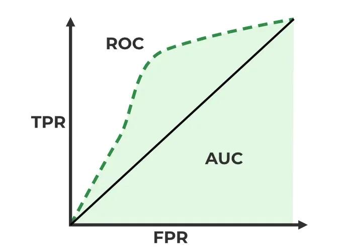
In diagnostic medicine, the Area Under the Receiver Operating Characteristic (ROC) Curve (AUC-ROC) quantifies the overall ability of a binary classifier to distinguish between two classes across all possible classification thresholds. The ROC curve itself plots the True Positive Rate (Sensitivity) against the False Positive Rate (1-Specificity) at various threshold settings [2]. The resulting AUC value provides a single measure of diagnostic performance that is threshold-independent, unlike sensitivity or specificity alone.
The interpretation of AUC values follows established standards:
- AUC = 0.5: Indicates no discriminative ability, equivalent to random guessing
- 0.5 < AUC < 0.7: Considered poor discriminative ability
- 0.7 ≤ AUC < 0.8: Acceptable discrimination
- 0.8 ≤ AUC < 0.9: Excellent discrimination
- AUC ≥ 0.9: Outstanding discrimination [2]
An AUC of 1.0 represents perfect classification, where the model achieves 100% sensitivity and 100% specificity simultaneously. The AUC equivalent to 0.5 indicates the classifier performs no better than chance in distinguishing between positive and negative cases.
Experimental Protocol: ROC Curve Generation and AUC Calculation
Purpose: To generate a Receiver Operating Characteristic (ROC) curve and calculate the Area Under the Curve (AUC) to evaluate the performance of a binary classification model.
Materials and Equipment:
- Dataset with known ground truth labels (positive/negative)
- Classification model producing probability scores
- Computational environment with statistical libraries (scikit-learn, pROC, etc.)
Procedure:
- Model Prediction: Obtain predicted probability scores for the positive class from your classification model on the test dataset.
- Threshold Definition: Define a series of classification thresholds ranging from 0 to 1 (typically 100+ increments).
- Classification at Thresholds: For each threshold:
- Convert probability scores to binary predictions (1 if ≥ threshold, 0 otherwise).
- Calculate True Positives (TP), False Positives (FP), True Negatives (TN), False Negatives (FN).
- Compute True Positive Rate: TPR = TP / (TP + FN).
- Compute False Positive Rate: FPR = FP / (FP + TN).
- ROC Plotting: Plot TPR against FPR for all thresholds to generate the ROC curve.
- AUC Calculation: Calculate the area under the ROC curve using numerical integration methods (e.g., trapezoidal rule) or dedicated functions (e.g.,
roc_auc_scorein scikit-learn) [2]. - Validation: Apply statistical methods to estimate confidence intervals for the AUC, typically through bootstrapping or DeLong's test for correlated ROC curves.
Implementation Note: Most statistical software packages provide built-in functions for ROC curve generation and AUC calculation. For example, Python's scikit-learn library includes roc_curve() and roc_auc_score() functions that automate steps 2-5 [2].
Diagnostic Performance of Biomarkers and Imaging Modalities
Table 2: Diagnostic accuracy of biomarkers and imaging modalities for various clinical conditions [3] [4]
| Biomarker/Modality | Clinical Application | Sensitivity (95% CI) | Specificity (95% CI) | AUC | Evidence Quality |
|---|---|---|---|---|---|
| Interleukin-6 (IL-6) | Late-onset neonatal sepsis | 85.2% (80.0-89.3%) | 84.1% (77.5-89.0%) | 0.91 | Moderate (GRADE) |
| Fecal Calprotectin (<50 μg/g) | Crohn's disease recurrence | 76% (70-82%) | 66% (56-75%) | 0.83* | Moderate |
| CT/MR Enterography | Crohn's disease recurrence | 89% (73-96%) | 65% (43-82%) | 0.87* | Moderate |
| Intestinal Ultrasound | Crohn's disease recurrence | 92% (75-96%) | 76% (52-90%) | 0.92* | Moderate |
| Note: AUC values marked with * are estimated from reported sensitivity and specificity values. IL-6 demonstrates excellent diagnostic accuracy (AUC 0.91) for late-onset neonatal sepsis, while cross-sectional imaging shows high sensitivity for detecting Crohn's disease recurrence. |
The Concordance Index (C-index) in Prognostic Research
Relationship Between AUC and C-index
The Concordance Index (C-index) represents an extension of the AUC principle to time-to-event data, making it particularly valuable for evaluating prognostic models in clinical research, especially in oncology. While standard AUC assesses discrimination in binary classification, the C-index measures the concordance between predicted risk scores and observed survival times, evaluating whether patients with higher risk scores experience events sooner than those with lower scores [5] [6] [7].
In practical applications, the C-index ranges from 0 to 1, with 0.5 indicating no predictive discrimination and 1.0 indicating perfect discrimination. Well-validated nomograms for cancer prognosis typically demonstrate C-index values between 0.70 and 0.85, reflecting moderate to strong predictive accuracy [5] [6] [7]. For example, a nomogram for early-stage cervical cancer achieved a C-index of 0.79 in the development cohort and 0.84 in the validation cohort for predicting disease-free survival [5], while a male breast cancer nomogram reported C-indices of 0.72-0.75 in internal validation and 0.98 in external validation [7].
Experimental Protocol: C-index Calculation for Prognostic Models
Purpose: To calculate the Concordance Index (C-index) for evaluating the discriminative ability of a prognostic model with time-to-event data.
Materials and Equipment:
- Dataset with observed survival times and event status
- Predicted risk scores from prognostic model
- Statistical software with survival analysis capabilities (R, Python, SPSS)
Procedure:
- Data Preparation: Compile dataset containing observed survival times, event indicators (1 for event, 0 for censored), and predicted risk scores for all subjects.
- Form All Comparable Pairs: Identify all possible pairs of subjects where the subject with shorter observed time experienced an event (i.e., not censored).
- Evaluate Concordance: For each comparable pair:
- Determine if the subject with higher risk score had the event first.
- Count the pair as concordant if higher risk score corresponds to earlier event.
- Count the pair as discordant if higher risk score corresponds to later event or no event.
- Count the pair as tied if risk scores are equal.
- Calculate C-index: Compute the C-index as (number of concordant pairs + 0.5 × number of tied pairs) / total number of comparable pairs.
- Validation: Assess statistical significance and calculate confidence intervals through bootstrapping or other resampling methods.
Implementation Note: Most statistical packages provide built-in functions for C-index calculation. In R, the coxph() function automatically computes the C-index for Cox models, while the concordance.index() function in various packages offers general calculation capabilities. Similar functionality exists in Python's lifelines library [5] [6] [7].
Research Reagent Solutions and Computational Tools
Table 3: Essential tools and resources for AUC and C-index research
| Tool/Resource | Primary Function | Application Context | Key Features |
|---|---|---|---|
| PlotDigitizer | Figure data extraction | Meta-analysis of published curves | Converts graph images to numerical data |
| R Statistical Software | Data analysis and modeling | AUC estimation, ROC analysis, C-index calculation | Comprehensive statistical packages (survival, rms, pROC) |
| Python Scikit-learn | Machine learning and evaluation | ROC curve generation, AUC calculation | roc_curve(), roc_auc_score() functions |
| SEER*Stat Software | Cancer database access | Prognostic model development | Population-based cancer incidence and survival data |
| X-tile Software | Cutpoint optimization | Risk stratification in prognostic models | Determines optimal cutoff values for continuous variables |
| PMC Literature Database | Scientific literature access | Methodological reference | Open-access biomedical literature |
| Note: These tools represent essential resources for researchers conducting AUC-related analyses, from data extraction to model development and validation. |
Area Under the Curve serves as a versatile quantitative metric with critical applications spanning pharmacokinetics and diagnostic medicine. In drug development, accurate AUC estimation through advanced methods like Monte Carlo simulation provides reliable quantification of drug exposure essential for dosage determination [1]. In diagnostic and prognostic research, AUC-ROC and C-index offer robust measures of discriminatory accuracy for classification models and survival predictions [5] [2] [6]. The methodological frameworks and experimental protocols presented in this article provide researchers with standardized approaches for implementing these analyses across diverse research contexts, ensuring rigorous quantitative assessment of biological responses and model performance.
Survival analysis, or time-to-event analysis, is a statistical method for analyzing the time until an event of interest occurs. A unique characteristic of survival data is censoring, where the event of interest is not observed for some subjects during the study period, meaning their true event times are only partially known [8] [9]. Evaluating predictive models in this context requires specialized metrics that account for this censoring, with the Concordance Index (C-index) emerging as the most commonly used metric for assessing the discriminatory power of survival models [8] [10].
The C-index measures a model's ability to produce a reliable ranking of subjects by their risk of experiencing an event. It represents the rank correlation between the predicted risk scores and the observed event times, quantifying the probability that the model orders any two comparable subjects correctly [8] [11] [10]. Unlike absolute accuracy measures which assess how close predictions are to actual values, the C-index evaluates ranking accuracy, making it particularly suitable for survival analysis where accurately identifying higher-risk versus lower-risk individuals is often the primary objective [12] [13].
Theoretical Foundations of the Concordance Index
Core Conceptual Framework
The fundamental intuition behind the C-index is that a good predictive model should assign higher risk scores to subjects who experience the event earlier than to those who experience it later or not at all [10]. Formally, for a pair of subjects (i, j), if subject i has a shorter observed survival time than subject j and also receives a higher risk score from the model, this pair is considered concordant. If the model assigns a lower risk score to the subject with the shorter survival time, the pair is discordant [8] [10].
The C-index is calculated as the ratio of concordant pairs to all comparable pairs [10]:
\begin{equation} C = \frac{\text{Number of concordant pairs} + \frac{1}{2} \times \text{Number of tied risk pairs}}{\text{Total number of comparable pairs}} \end{equation}
Ties in risk scores are typically counted as half-concordant [13]. The resulting value ranges from 0 to 1, where 0.5 indicates predictions no better than random chance, and 1 represents perfect discrimination [10].
Handling Censored Data
A particular challenge in survival analysis is determining which pairs of subjects are comparable given the presence of censoring [8] [10]. The handling of different types of pairs is summarized below:
Table 1: Handling of Different Types of Subject Pairs in C-index Calculation
| Pair Type | Description | Treatment in C-index |
|---|---|---|
| Both subjects experienced event | Known ordering of event times | Always comparable |
| One censored, one with event | Comparable only if event time < censoring time | Included only if ordering is known |
| Both subjects censored | Unknown which would experience event first | Not comparable (excluded) |
| Tied risk scores | Model assigns equal risk to both subjects | Counted as half-concordant |
[8] [10] [13] provides a clear example: if a subject experienced an event at time t = 3 years, and another subject was censored at t = 5 years, we know the first subject experienced the event first, making this pair comparable. If instead the censoring occurred at t = 2 years, we cannot determine who would have experienced the event first, making the pair non-comparable [13].
Quantitative Comparison of Concordance Index Variants
Key C-index Estimators and Their Properties
Several statistical estimators have been developed to calculate the C-index, each with different properties and suitability for various research contexts.
Table 2: Comparison of Major C-index Estimators in Survival Analysis
| Estimator | Key Principle | Advantages | Limitations | Suitable Contexts |
|---|---|---|---|---|
| Harrell's C-index [14] [10] [9] | Direct comparison of comparable pairs | Intuitive; easy to compute; widely used | Optimistic bias with high censoring; depends on censoring distribution | Low censoring rates; preliminary analysis |
| Uno's C-index [8] [14] | Inverse probability of censoring weighting (IPCW) | Less biased with high censoring; robust to independent censoring | Requires correct censoring model; still biased with dependent censoring | High censoring rates with independent censoring |
| Gerds' C-index [14] | IPCW with covariate-dependent censoring | Handles policy-related dependent censoring; more appropriate for policy evaluation | Complex implementation; requires modeling censoring distribution | Policy evaluations; dependent censoring scenarios |
Impact of Censoring on Different Estimators
The performance of these estimators varies significantly based on the censoring mechanism and rate. Simulation studies have demonstrated that Harrell's C-index becomes increasingly optimistic as censoring rates increase, while Uno's estimator remains more stable under independent censoring [8]. In policy-sensitive contexts where censoring depends on risk scores (e.g., patients with higher scores receive interventions and become censored), only Gerds' C-index appropriately accounts for this dependency [14].
Experimental Protocols for C-index Evaluation
Standard Protocol for Calculating Harrell's C-index
Objective: To evaluate the performance of a survival prediction model using Harrell's C-index.
Materials and Reagents:
- Dataset: Survival data containing observed times and event indicators for all subjects
- Software: Statistical software with survival analysis capabilities (e.g., R survival package, scikit-survival, lifelines, PySurvival)
- Model: Trained survival prediction model capable of generating risk scores
Procedure:
- Generate risk scores: Use the trained model to compute a risk score for each subject in the dataset
- Identify comparable pairs: For each unique pair of subjects (i, j), determine if they are comparable based on event times and censoring status
- Classify pairs: For each comparable pair:
- If risk score i > risk score j and time i < time j → Concordant pair
- If risk score i < risk score j and time i < time j → Discordant pair
- If risk score i = risk score j → Tied risk pair
- Calculate C-index: Apply the formula to compute the final concordance statistic
- Interpret results: Values closer to 1.0 indicate better discrimination performance
Protocol for Handling Dependent Censoring with Gerds' C-index
Objective: To evaluate model performance when censoring is dependent on risk scores.
Additional Materials:
- Censoring model: Methodology to estimate censoring probabilities based on covariates
Procedure:
- Model the censoring distribution: Estimate probabilities of being censored at each time point using a regression model that incorporates risk scores and other relevant covariates
- Calculate inverse probability weights: Compute weights for each subject based on the estimated probability of remaining uncensored
- Apply weighted comparison: Compare subject pairs using these weights to account for differential censoring patterns
- Compute weighted C-index: Calculate the concordance statistic using the weighted contributions of each comparable pair
Validation Protocol for C-index Stability
Objective: To assess the stability of C-index estimates across different censoring patterns.
Procedure:
- Apply synthetic censoring: Artificially introduce additional censoring into the dataset using specified mechanisms (independent, risk-dependent)
- Compute multiple C-indices: Calculate Harrell's, Uno's, and Gerds' C-indices on the synthetically censored data
- Compare results: Analyze how each estimator behaves under different censoring scenarios
- Assess robustness: Determine which estimator provides the most stable performance across censoring patterns
Visualization of C-index Concepts and Workflows
Logical Flow for Concordance Assessment
Diagram 1: C-index Calculation Workflow - This diagram illustrates the logical decision process for classifying subject pairs when calculating the C-index, showing how comparable pairs are identified and classified as concordant, discordant, or tied.
Experimental Framework for Method Comparison
Diagram 2: C-index Comparison Protocol - This workflow shows the experimental process for comparing different C-index estimators on the same dataset and model, highlighting the parallel calculation of different variants.
The Scientist's Toolkit: Essential Research Reagents
Table 3: Essential Computational Tools for C-index Research
| Tool/Reagent | Function | Implementation Considerations |
|---|---|---|
| scikit-survival [8] [13] | Python library for survival analysis | Provides concordanceindexcensored(), concordanceindexipcw(); uses predicted risks |
| lifelines [13] | Python survival analysis library | Concordance index based on predicted event times rather than risks |
| PySurvival [11] [13] | Python survival modeling framework | concordance_index() function requires model object input |
| survival (R package) [10] [15] | Comprehensive survival analysis in R | Standard for statistical validation; widely cited in literature |
| Simulated datasets [8] | Method validation | Generate data with known censoring mechanisms to test estimator robustness |
A critical note for researchers: different software packages may implement the C-index with subtle variations. For instance, scikit-survival expects predicted risks (higher value = higher risk), while lifelines uses predicted event times (higher value = longer survival). This means that for the same model, the C-index in scikit-survival will typically equal 1 - C-index in lifelines [13]. PySurvival additionally counts subject pairs in both directions (both (i,j) and (j,i)), effectively doubling the number of pairs compared to other implementations [13]. These differences must be accounted for when comparing results across studies or software platforms.
Advanced Applications and Recent Methodological Developments
C-index Decomposition for Model Insight
Recent research has proposed decomposing the C-index into components that provide deeper insights into model performance. The overall C-index can be expressed as a weighted harmonic mean of two quantities:
- CI~ee~: Ranking of observed events versus other observed events
- CI~ec~: Ranking of observed events versus censored cases [9]
This decomposition reveals that different models may perform differently on these two aspects, explaining why some models maintain stable performance across censoring levels while others deteriorate. Deep learning models, for instance, have been shown to utilize observed events more effectively than classical methods, maintaining stable C-indices across different censoring levels [9].
Time-Dependent Extensions
For applications where predictive performance within specific time horizons is important, time-dependent extensions of the C-index have been developed. These are closely related to time-dependent ROC curves and evaluate how well a model distinguishes between subjects who experience an event by a given time from those who do not [8] [16]. The cumulative/dynamic AUC implemented in scikit-survival's cumulative_dynamic_auc() function addresses this need for time-specific discrimination assessment [8].
The Concordance Index remains a fundamental metric for evaluating predictive performance in survival analysis, with multiple estimators available to address different research contexts and censoring mechanisms. Proper application requires understanding the censoring mechanisms in the data, selecting the appropriate estimator, and being aware of implementation differences across software platforms. Recent methodological developments, including decomposition approaches and time-dependent extensions, continue to enhance the depth of insight that can be gained from this versatile metric. As survival modeling increasingly incorporates machine learning approaches, appropriate use of the C-index and its variants will remain essential for rigorous model evaluation and comparison.
The Fundamental Relationship Between AUC and Harrell's C-index
Within the realms of machine learning, medical statistics, and survival analysis, researchers and drug development professionals frequently require robust metrics to evaluate the performance of predictive models. For binary classification tasks, the Area Under the Receiver Operating Characteristic Curve (AUC) is the standard measure of a model's ability to discriminate between classes [17]. In time-to-event analyses, which are crucial for clinical trials and drug development, Harrell's C-index (or concordance index) is the predominant metric for assessing a model's ability to rank survival times [10]. A clear understanding of the fundamental relationship between these two metrics is essential for the proper validation of prognostic models. This application note delineates this relationship, provides protocols for their computation, and discusses their appropriate application within a research context, particularly for drug development.
Theoretical Foundations and Definitions
Area Under the Curve (AUC)
The AUC is a performance measurement for classification problems at various threshold settings. It is derived from the Receiver Operating Characteristic (ROC) curve, which plots the True Positive Rate (TPR or Sensitivity) against the False Positive Rate (FPR or 1-Specificity) across all possible classification thresholds [17].
- Interpretation: The AUC represents the probability that a randomly selected positive instance will be ranked higher than a randomly selected negative instance by the model. An AUC of 1.0 signifies perfect discrimination, 0.5 indicates performance no better than random chance, and values below 0.5 suggest worse-than-chance performance [17].
- Formula Context: For a binary outcome ( D ) and a model score ( M ), the AUC is defined as ( P(M{diseased} > M{non-diseased}) ) [16].
Harrell's C-index
Harrell's C-index evaluates a model's ability to produce a risk score that correctly orders subjects by their time until an event [10]. It is essential for censored survival data, where the exact event time is not known for all subjects.
- Core Concept: The C-index is the proportion of all usable pairs of subjects where the model's predictions and the actual outcomes are concordant [10].
- Permissible Pairs: A pair of subjects is considered "permissible" or "usable" only if the order of their event times can be unequivocally determined. This typically excludes pairs where both subjects are censored or where a censored subject's event time precedes the observed event time of another [10] [18].
- Calculation: The simplified C-index is calculated as: ( C = \frac{\text{Number of Concordant Pairs}}{\text{Number of Permissible Pairs}} ) Tied risk scores are often accounted for by adding half the number of tied pairs to the numerator [18].
- Interpretation: A C-index of 1 indicates perfect concordance, 0.5 suggests no better than random ordering, and 0 indicates perfect discordance [10].
The following diagram illustrates the logical relationship between AUC and the C-index, and the workflow for calculating the C-index.
The Fundamental Relationship
The relationship between AUC and Harrell's C-index is one of conceptual generalization.
For a binary outcome, the C-index is mathematically equivalent to the AUC [19] [20]. In this specific scenario, the "positive" and "negative" instances form the permissible pairs, and concordance is achieved when the positive instance receives a higher risk score.
Harrell's C-index generalizes the concept of the AUC to survival data, where outcomes are time-to-event and subject to censoring [20]. While the standard AUC is static, the C-index dynamically accounts for whether a subject with a higher risk score experiences the event before a subject with a lower risk score, considering the complexities introduced by censored observations. The concordance matrix used to compute the C-index for a binary classifier directly corresponds to the ROC curve, and the area under this curve is the AUC [20].
Table 1: Key Characteristics of AUC and Harrell's C-index
| Feature | AUC (for Binary Outcomes) | Harrell's C-index (for Survival Outcomes) |
|---|---|---|
| Outcome Type | Binary (e.g., disease/no disease) | Time-to-event with censoring |
| Core Question | Does the model rank a random positive higher than a random negative? | Does the model rank a random shorter survivor higher than a random longer survivor? |
| Pair Usage | All case-vs-control pairs are used [18] | Only "permissible" pairs are used (handles censoring) [10] |
| Theoretical Relationship | Base metric for binary classification | A generalization of AUC to survival data [20] |
Calculation Protocols
Protocol for Calculating AUC
This protocol outlines the steps for calculating the AUC for a binary classifier.
1. Problem Definition: Define a binary classification task (e.g., predicting responders vs. non-responders to a drug therapy).
2. Model and Scores: Train a predictive model (e.g., logistic regression, random forest) that outputs a continuous score or probability for the positive class for each subject.
3. Vary Thresholds: Systematically vary the classification threshold from the minimum to the maximum predicted score.
4. Calculate TPR and FPR: At each threshold, calculate the True Positive Rate (TPR) and False Positive Rate (FPR) using the confusion matrix.
- ( TPR = \frac{TP}{TP + FN} )
- ( FPR = \frac{FP}{FP + TN} )
5. Plot ROC Curve: Graph the resulting (FPR, TPR) pairs.
6. Calculate AUC: Compute the area under the plotted ROC curve using a numerical integration method such as the trapezoidal rule [17].
Protocol for Calculating Harrell's C-index
This protocol is designed for evaluating a Cox proportional hazards or other survival model in a clinical study setting.
1. Study Data Preparation: Collect time-to-event data, including covariates, observed time ((Xi)), and event indicator ((\Deltai)).
2. Survival Model Fitting: Fit a survival model (e.g., Cox PH model) to the data to obtain a risk score ((\etai = \mathbf{Zi}^\top \boldsymbol{\beta})) for each subject.
3. Identify All Pairs: Enumerate all possible pairs of subjects ((i, j)).
4. Classify Pairs: For each pair, determine if it is permissible and, if so, whether it is concordant. The decision logic is summarized in the table below.
Table 2: Classification of Subject Pairs for Harrell's C-index
| Case | Subject i | Subject j | Permissible? | Concordant if |
|---|---|---|---|---|
| 1 | Event at (T_i) | Event at (T_j) | Yes | ( \etai > \etaj ) and ( Ti < Tj ) [10] |
| 2 | Censored at (T_i) | Censored at (T_j) | No | - |
| 3 | Event at (T_i) | Censored at (T_j) | Only if ( Ti < Tj ) [10] | ( \etai > \etaj ) |
| 4 | Censored at (T_i) | Event at (T_j) | Only if ( Tj < Ti ) [10] | ( \etaj > \etai ) |
5. Compute C-index: Tally the total number of concordant pairs and permissible pairs. Apply the formula: ( C = \frac{\text{Number of Concordant Pairs} + 0.5 \times \text{Number of Tied Risk Pairs}}{\text{Number of Permissible Pairs}} ) [18].
The following workflow diagram visualizes the computational steps for Harrell's C-index.
The Scientist's Toolkit: Key Reagents and Computational Solutions
Table 3: Essential Materials and Tools for AUC and C-index Research
| Item / Solution | Function / Description | Example / Note |
|---|---|---|
| Time-to-Event Dataset | The fundamental input for survival model development and C-index validation. Must include time-to-event, censoring indicator, and covariates. | Clinical trial data with overall survival (OS) or progression-free survival (PFS) endpoints. |
| Binary Outcome Dataset | The fundamental input for binary classifier development and AUC calculation. | Data from a diagnostic test study with confirmed disease status. |
| Statistical Software (R/Python) | Provides environments with comprehensive packages for calculating both AUC and C-index. | R: survival package (concordance), pROC package (AUC). Python: scikit-survival (C-index), scikit-learn (AUC). |
| Phoenix WinNonlin | A commercial software platform used in pharmacokinetics/pharmacodynamics (PK/PD) for non-compartmental analysis (NCA), which calculates AUC for drug concentration-time curves [21]. | Uses methods like Linear-Log Trapezoidal for calculating exposure metrics like AUC0-inf [21] [22]. |
| Inverse Probability Weighting (IPW) | A statistical technique used to make C-index estimates more robust to censoring patterns, ensuring they are less dependent on the study-specific censoring distribution [23]. | Used in advanced C-statistics to create estimators that are consistent for a population parameter free of censoring [23]. |
Advanced Considerations and Limitations
While Harrell's C-index is immensely useful, researchers must be aware of its limitations. The standard C-index can be sensitive to the study-specific censoring distribution [23]. Modifications, such as Uno's C-index or IPW-based estimators, have been developed to provide a measure that is less dependent on the censoring pattern [23]. Furthermore, the C-index has been criticized for its insensitivity to the addition of new, significant predictors to a model and for its focus on the ranking of pairs rather than the absolute accuracy of predictions [18]. For a more granular assessment, time-dependent AUC methods can evaluate discrimination at specific time points (e.g., 1-year, 5-year) and can be connected to the C-index as a weighted average of these time-specific AUCs [16].
Pharmacokinetic Studies: Quantifying Drug Exposure
Core Principles and Calculation Methods
The Area Under the Curve (AUC) in pharmacokinetics (PK) represents the integral of a substance's plasma concentration over time, serving as a crucial indicator of total drug exposure within the body [24]. Expressed in units such as mg·h/L, AUC is derived from concentration-time data established during pharmacokinetic studies and is essential for evaluating medication bioavailability [24]. This metric quantifies how much of a substance reaches systemic circulation and its potential therapeutic effects, making it fundamental for dose selection and therapeutic monitoring [24].
Table 1: AUC Calculation Methods in Pharmacokinetics
| Method | Formula | Application Context | Advantages/Limitations |
|---|---|---|---|
| Linear Trapezoidal | AUC = Σ [0.5 × (C₁ + C₂) × (t₂ - t₁)] |
General use; increasing concentrations | Simple calculation; may overestimate AUC during elimination phase [21] |
| Logarithmic Trapezoidal | AUC = (t₂ - t₁) × (C₁ - C₂)/ln(C₁/C₂) |
Decreasing concentrations (elimination phase) | More accurate for exponential elimination; assumes C₁ > C₂ [21] [22] |
| Linear-Log Trapezoidal (Linear-Up Log-Down) | Combination: Linear for increasing concentrations, Log for decreasing concentrations | Complete concentration-time profiles | Most accurate overall; appropriate for both absorption and elimination phases [21] |
| AUC Extrapolation to Infinity | AUC₀‑inf = AUC₀‑last + Cₚₜ/Kₑₗ |
Complete exposure estimation | Provides total drug exposure; requires accurate determination of elimination rate constant (Kₑₗ) [22] |
Advanced Considerations: Accounting for Variable Baselines
In specialized applications such as gene expression data or pharmacodynamic responses, the initial condition for the response of interest is often not zero, creating uncertainty in the true baseline value [25]. This necessitates calculating AUC relative to a variable baseline, which accounts for inherent uncertainty and variability in baseline measurements [25]. The algorithm involves:
Estimating Baseline and Its Error: Depending on experimental design, baseline can be estimated from:
- Measurements at only t=0 (for chronic dosing scenarios)
- Measurements at t=0 and t=Tₗₐₛₜ (for acute dosing with return to baseline)
- Separate control group measurements at each time point (for circadian rhythms or other variable baselines) [25]
Estimating AUC and Its Error: Using bootstrapping approaches with the trapezoidal rule applied to resampled data [25].
Handling Biphasic Responses: Calculating positive and negative AUC components separately to identify multiphasic responses where values deviate both above and below baseline [25].
AUC Calculation Decision Framework
Experimental Protocol: AUC Determination in Preclinical PK Studies
Objective: To determine the pharmacokinetic profile and total exposure of a novel compound following intravenous administration to rat models.
Materials and Reagents:
- Test compound (≥95% purity)
- Sprague-Dawley rats (250-300 g, n=6 per group)
- Heparinized blood collection tubes
- LC-MS/MS system for compound quantification
- Phoenix WinNonlin software for PK analysis
Procedure:
- Dose Administration: Administer 5 mg/kg test compound via tail vein injection.
- Blood Sampling: Collect serial blood samples (0.3 mL) at pre-dose, 0.08, 0.25, 0.5, 1, 2, 4, 8, 12, and 24 hours post-dose.
- Sample Processing: Immediately centrifuge samples at 4°C, 3000 × g for 10 minutes. Transfer plasma to clean tubes and store at -80°C until analysis.
- Bioanalysis: Quantify compound concentrations using validated LC-MS/MS method with calibration standards (1-1000 ng/mL).
- Data Analysis:
- Calculate mean concentration at each time point
- Apply linear-up log-down trapezoidal method to calculate AUC₀‑t
- Determine terminal elimination rate constant (Kₑₗ) from log-linear regression of the last 4-5 time points
- Calculate AUC₀‑inf = AUC₀‑t + Cₗₐₛₜ/Kₑₗ
- Report mean ± SD AUC values across subjects
Quality Control: Include quality control samples at low, medium, and high concentrations during bioanalysis with acceptance criteria of ±15% deviation from nominal values.
Bioequivalence Trials: Establishing Therapeutic Equivalence
Regulatory Framework and Acceptance Criteria
Bioequivalence (BE) trials are abbreviated clinical studies that evaluate whether a generic drug or new formulation is equivalent to a previously approved reference product [26]. These trials rely primarily on AUC and Cₘₐₓ (maximum plasma concentration) as key parameters for comparing the extent and rate of absorption, respectively [27]. The current FDA guidelines declare products average bioequivalent if the difference in their population means on the log-transformed scale falls within the regulatory limit of ±0.223, corresponding to the 80-125% equivalence range in the original scale [26].
Table 2: Bioequivalence Assessment Approaches
| Approach | Statistical Criteria | Application Context | Regulatory Requirements |
|---|---|---|---|
| Average Bioequivalence (ABE) | 90% CI for GMR (T/R) must fall within 80-125% [27] | Standard drugs with low to moderate variability | Standard 2x2 crossover design; 12-24 subjects typically |
| Reference-Scaled Average Bioequivalence (RSABE) | Acceptance range widens based on reference variability: [exp(∓k × sWR)] where k=0.294 (EMA) or 0.25 (FDA) [27] |
Highly variable drugs (CV ≥30%) [27] | Replicated crossover design; reference administered at least twice; ≥24 subjects (FDA) |
| Population Bioequivalence | Comparison of total variability (within + between subject) | Ensuring switchability between populations | More complex study designs; not routinely required |
| Individual Bioequivalence | Comparison within-subject variances | Assessing switchability for individuals | Most complex; rarely required in practice |
Advanced Methodology: RSABE for Highly Variable Drugs
For highly variable drugs (HVDs) with within-subject coefficient of variation ≥30%, the Reference-Scaled Average Bioequivalence approach has been adopted to address the challenge of demonstrating bioequivalence [27]. The high intra-subject variability can obscure real similarities between products, making traditional ABE approaches impractical due to the excessively large sample sizes that would be required [27].
The RSABE methodology scales the bioequivalence limits according to the within-subject variability of the reference product:
EMA RSABE Equation:
-ln(1.25) × (SWR/0.294) ≤ μT - μR ≤ ln(1.25) × (SWR/0.294)
FDA RSABE Equation:
-ln(1.25) × (SWR/0.25) ≤ μT - μR ≤ ln(1.25) × (SWR/0.25)
Where SWR is the within-subject standard deviation of the reference product, and μT - μR is the difference between logarithmic means of test and reference products [27].
Table 3: RSABE Acceptance Range at Different Variability Levels
| Within-Subject CV (%) | SWR | EMA RSABE Limits | FDA RSABE Limits |
|---|---|---|---|
| 30 | 0.294 | 80.00 - 125.00 | 76.94 - 129.97 |
| 40 | 0.385 | 74.62 - 134.02 | 70.89 - 141.06 |
| 50 | 0.472 | 69.84 - 143.19 | 65.58 - 152.48 |
| 60 | 0.555 | 69.84 - 143.19 (max) | 60.95 - 164.08 |
Experimental Protocol: Two-Period Crossover Bioequivalence Study
Objective: To demonstrate bioequivalence between a test formulation and reference listed drug.
Study Design: Randomized, two-period, two-sequence, single-dose crossover with ≥14-day washout period.
Subjects: Healthy adult volunteers (n=24), 18-55 years, BMI 18.5-30 kg/m², confirmed health status through medical history, physical examination, and laboratory tests.
Procedures:
- Screening: Informed consent; eligibility assessment within 21 days prior to dosing.
- Period 1: Overnight fasting (≥10 hours); administer single dose with 240 mL water; standardized meals at 4 and 10 hours post-dose.
- Blood Sampling: Pre-dose and at 0.25, 0.5, 0.75, 1, 1.5, 2, 2.5, 3, 4, 6, 8, 12, 16, 24, 36, and 48 hours post-dose.
- Washout: 14-day period based on 5× terminal half-life of reference drug.
- Period 2: Repeat procedures with alternate formulation.
Bioanalytical Method:
- Validated LC-MS/MS method per FDA guidance
- Calibration range covering expected concentrations
- Quality controls (low, medium, high) with ≤15% deviation
Statistical Analysis:
- Calculate AUC₀‑t, AUC₀‑inf, and Cₘₐₓ for both formulations
- ANOVA on log-transformed parameters including sequence, period, and treatment effects
- Construct 90% confidence intervals for geometric mean ratio (Test/Reference)
- Conclude bioequivalence if 90% CI falls within 80-125% for all primary parameters
Survival Model Evaluation: Moving Beyond the C-index
Limitations of Concordance Index in Survival Analysis
The concordance index (C-index) measures the rank correlation between predicted risk scores and observed event times, representing the ratio of correctly ordered pairs to comparable pairs [8]. Despite its widespread use (employed in over 80% of survival analysis studies in leading statistical journals), the C-index has significant limitations [28]:
- Insensitivity to clinically significant predictors: The C-index may show minimal improvement even when statistically and clinically significant covariates are added to models [28].
- Dependence only on ranks: Models with inaccurate survival predictions can have higher C-indices than models with more accurate predictions due to the metric's reliance solely on ranking [28].
- Optimistic bias with high censoring: Harrell's C-index has been shown to be overly optimistic with increasing amounts of censored data [8].
- Limited clinical relevance: In low-risk populations, the C-index often compares patients with very similar risk probabilities, providing little practical value to clinicians [28].
Comprehensive Survival Model Evaluation Framework
A robust evaluation strategy for survival models should incorporate multiple metrics addressing different aspects of model performance:
Table 4: Survival Model Evaluation Metrics
| Metric | Formula/Calculation | Interpretation | Strengths/Limitations |
|---|---|---|---|
| Harrell's C-index | C = (Concordant Pairs + 0.5 × Tied Pairs)/Comparable Pairs |
Probability that predictions correctly rank order survival times | Intuitive; widely used; but optimistic with high censoring [8] |
| IPCW C-index | Inverse Probability of Censoring Weighting | Less biased estimate of concordance | Addresses censoring bias; more appropriate with high censoring [8] |
| Integrated Brier Score | IBS = 1/τ × ∫₀τ BS(t) dt where BS(t) = 1/N × Σ[(0 - S(t⎪x))² × I(t ≤ y, δ=1) + (1 - S(t⎪x))² × I(t > y)] |
Overall measure of prediction error (0-1 scale) | Assesses both discrimination and calibration; lower values indicate better performance [8] |
| Restricted AUC | AUC = ∫₀τ S(t) dt where S(t) is survival function |
Mean survival time up to time τ | Captures survival plateau; model-independent calculation [29] |
| Time-Dependent AUC | AUC(t) = P(Ŝᵢ(t) < Ŝⱼ(t) ⎪ Tᵢ ≤ t, Tⱼ > t) |
Discrimination at specific time points | Identifies time-varying discrimination performance [8] |
The AUC Method for Survival Curve Analysis
In survival analysis, the area under the survival curve provides a valuable alternative to median survival, particularly for detecting survival plateaus that often occur with immunotherapies and other novel cancer treatments [29]. The AUC method essentially represents a rearrangement of traditional mean lifetime survival measures [29].
Key Applications:
- Randomized Controlled Trials: The ratio between AUC values in treatment and control groups provides information similar to the hazard ratio while better capturing long-term survival differences [29].
- Single-Arm Trials: The ratio between AUC and median survival identifies long-term survival plateaus (ratio >1 indicates presence of plateau) [29].
Calculation Method:
- Restricted AUC (rAUC): Calculated from time zero to the last observed time-point using the trapezoidal rule applied to the Kaplan-Meier survival curve [29].
- Unrestricted AUC: Extrapolated to infinity using model-based approaches (e.g., Weibull, Gompertz distributions) [29].
Survival Model Evaluation Framework
Experimental Protocol: Comprehensive Survival Model Validation
Objective: To evaluate the performance of a novel survival prediction model for overall survival in advanced non-small cell lung cancer patients.
Data:
- Training set: n=1,500 patients with clinical, genomic, and treatment data
- Validation set: n=500 patients from different institutions
- Primary endpoint: Overall survival from diagnosis to death from any cause
Evaluation Procedure:
- Model Training: Develop Cox proportional hazards model with regularization to predict survival distributions.
- Discrimination Assessment:
- Calculate Harrell's C-index and IPCW C-index on validation set
- Compute time-dependent AUC at 1, 2, and 3 years
- Compare concordance between risk groups
- Calibration Assessment:
- Calculate integrated Brier score over observed time range
- Create calibration plots comparing predicted vs observed survival at 1, 2, and 3 years
- Perform Hosmer-Lemeshow-type tests for survival models
- Clinical Utility Assessment:
- Calculate restricted AUC (rAUC) up to 5 years for each treatment group
- Perform milestone analysis at 2 and 3 years
- Compare AUC/median ratios to identify survival plateaus
- Comparison to Benchmarks:
- Compare all metrics against established clinical prognostic scores
- Perform statistical tests for differences in performance metrics
Reporting: Present all metrics with confidence intervals and clinical interpretations of observed differences.
Research Reagent Solutions
Table 5: Essential Tools for AUC and Survival Analysis
| Category | Specific Tools/Software | Primary Application | Key Features |
|---|---|---|---|
| PK/PD Analysis Software | Phoenix WinNonlin [21] [27] | Noncompartmental analysis for bioavailability studies | Implements multiple AUC methods; RSABE templates; regulatory-compliant output |
| Statistical Programming | R Survival package; scikit-survival [8] | Survival model development and evaluation | Implements C-index, IPCW C-index, time-dependent AUC, Brier score |
| Bioanalytical Instruments | LC-MS/MS systems with validated methods | Drug concentration quantification | High sensitivity and specificity for PK studies; required for BE trials |
| Clinical Data Management | Electronic Data Capture (EDC) systems | BE trial and survival study data collection | 21 CFR Part 11 compliance; audit trails; data integrity |
| Study Design Templates | FDA/EMA RSABE project templates [27] | Highly variable drug bioequivalence studies | Predefined analysis workflows for regulatory submissions |
Area Under the Curve (AUC) serves as a fundamental pharmacokinetic (PK) parameter that quantifies total systemic drug exposure over time [21]. In drug development, accurate AUC calculation is critical for assessing bioavailability, determining dosing regimens, and establishing bioequivalence between drug formulations [21]. The implementation of robust AUC methodologies must align with regulatory standards, particularly the ICH Q2(R2) guideline on analytical procedure validation, which emphasizes parameters such as accuracy, precision, specificity, and linearity in analytical measurements [30]. This framework ensures that the AUC data generated throughout drug development possesses the necessary quality and reliability to support regulatory submissions and clinical decision-making.
Beyond traditional pharmacokinetics, AUC has significant applications in machine learning for evaluating classification models [17] and in survival analysis through related concordance indices [31] [28]. The convergence of these methodologies in modern drug development requires researchers to understand both the computational techniques and appropriate contexts for their application. This document provides comprehensive application notes and experimental protocols for AUC implementation within this broad regulatory and methodological context, serving the needs of researchers, scientists, and drug development professionals engaged in quantitative analysis.
AUC Calculation Methods: Theory and Applications
Fundamental Trapezoidal Methods for AUC Calculation
The trapezoidal family of methods forms the foundation for numerical AUC estimation in pharmacokinetic analysis, each with distinct mathematical approaches and applications.
Linear Trapezoidal Method: This approach applies linear interpolation between concentration-time data points, forming trapezoids whose areas are summed to calculate total AUC [21]. For a time interval (t₁ to t₂), the AUC is calculated as: AUC = (C₁ + C₂)/2 × (t₂ - t₁), where C₁ and C₂ are consecutive concentration measurements [21]. While mathematically straightforward, this method can overestimate AUC during the elimination phase because it does not account for the exponential nature of drug concentration decline [21].
Logarithmic Trapezoidal Method: This method uses logarithmic interpolation between concentration-time points, making it particularly suitable for decreasing concentrations that follow first-order elimination kinetics [21]. The formula for a given interval is: AUC = (C₁ - C₂)/(ln(C₁) - ln(C₂)) × (t₂ - t₁) [21]. This approach more accurately captures the exponential decay characteristic of drug elimination but may underestimate AUC during absorption phases [21].
Linear-Log Trapezoidal Method (Linear-Up/Log-Down): This hybrid approach applies the linear trapezoidal method when concentrations are increasing (absorption phase) and the logarithmic method when concentrations are decreasing (elimination phase) [21]. Recognized as one of the most accurate numerical methods for AUC estimation, it effectively models both the ascending and descending portions of the concentration-time profile [21]. Phoenix WinNonlin implements this as the "Linear Up Log Down" method, which does not depend solely on Cmax, making it suitable for profiles with secondary peaks [21].
Table 1: Comparison of Primary AUC Calculation Methods
| Method | Mathematical Basis | Optimal Application Phase | Advantages | Limitations |
|---|---|---|---|---|
| Linear Trapezoidal | Linear interpolation | Absorption phase | Simple implementation; intuitive calculation | Overestimates elimination phase AUC |
| Logarithmic Trapezoidal | Logarithmic interpolation | Elimination phase | Accurate for exponential decay | Underestimates absorption phase AUC |
| Linear-Log Trapezoidal (Linear-Up/Log-Down) | Combines linear and logarithmic approaches | Entire concentration-time profile | Most accurate overall; adapts to curve shape | More complex implementation |
| Bayesian Estimation | Population PK with Bayesian priors | Early therapy; sparse sampling | Reduces sampling burden; enables early optimization | High cost; model variability [32] |
Advanced AUC Estimation Methods
Beyond traditional trapezoidal methods, advanced approaches have been developed for specific applications:
First-Order Pharmacokinetic Equations: These methods utilize timed post-infusion drug levels to estimate patient-specific PK parameters and AUC [32]. The trapezoidal PK equation approach computes daily AUC (AUC₂₄) using the formula: AUC₂₄ = (AUCᵢₙf + AUCₑₗᵢₘ) × (24/Tau), where AUCᵢₙf represents the area under the infusion curve (Tᵢₙf × 0.5 × (Cmax + Cmin)) and AUCₑₗᵢₘ describes the area under the elimination curve ((Cmax - Cmin)/Kₑₗ) [32]. This method provides accurate, patient-specific AUC estimates with minimal assumptions but offers static estimates that require new concentration measurements when patient physiology changes [32].
Bayesian Methods: These approaches apply Bayesian statistical theory to integrate population pharmacokinetic data (prior) with patient-specific drug levels and clinical parameters (posterior) [32]. This iterative mathematical approach provides refined AUC estimates and dosing recommendations, with the significant advantage of enabling early AUC optimization using pre-steady-state levels and reducing sampling burden [32]. Limitations include high implementation costs and variability in accuracy between different commercially available software platforms [32].
Concordance Index Research and Applications
Concordance Index Fundamentals
The Concordance Index (C-index) serves as a crucial performance metric in survival analysis and risk prediction models, evaluating a model's ability to correctly rank order survival times [28]. In essence, the C-index measures the probability that, for two randomly selected patients, the patient with higher predicted risk will experience the event first [28]. This ranking metric has become particularly important in healthcare applications such as evaluating risk prediction models for hospital readmission, cardiovascular disease, and treatment-related complications [31].
Despite its widespread adoption, with over 80% of survival analysis studies in leading statistical journals using C-index as their primary evaluation metric, significant limitations have been identified [28]. The C-index measures only discriminative ability (ranking) without assessing the accuracy of time-to-event predictions or the calibration of probabilistic estimates [28]. It demonstrates insensitivity to the addition of clinically significant covariates and can provide misleadingly high values in low-risk populations where patients have similar risk profiles [28].
Advanced Concordance Index Methodologies
Recent research has addressed limitations in traditional concordance metrics through methodological refinements:
C-index Decomposition: A novel approach decomposes the C-index into a weighted harmonic mean of two components: (1) the C-index for ranking observed events versus other observed events, and (2) the C-index for ranking observed events versus censored cases [33]. This decomposition enables finer-grained analysis of model performance, revealing that deep learning models utilize observed events more effectively than classical methods, maintaining stable C-index performance across varying censoring levels [33].
Gerds' Weighting: This advanced weighting scheme addresses deficiencies in standard C-index methodologies under policy-related dependent censoring [31]. In comparative studies of liver failure patients, the concordance metric based on Gerds' weighting demonstrated different performance characteristics (0.864, 95% CI: 0.840-0.888) compared to Harrell's C-Index (0.854, 95% CI: 0.844-0.864) and Uno's C-Index (0.832, 95% CI: 0.819-0.844) when evaluating Model for End-Stage Liver Disease (MELD) scores [31]. This highlights the importance of selecting appropriate weighting schemes to avoid bias in policy evaluations.
Table 2: Comparison of Concordance Index Methodologies
| Metric | Statistical Basis | Censoring Handling | Applications | Key Considerations |
|---|---|---|---|---|
| Harrell's C-Index | Proportional hazards assumptions | Handles right-censoring | General survival analysis | Standard approach; may be insensitive to new covariates [28] |
| Uno's C-Index | Inverse probability weighting | More robust to censoring distribution | Studies with non-random censoring | Improved performance with informative censoring |
| Gerds' Weighting | Inverse probability of censoring weights | Addresses dependent censoring | Policy evaluation; healthcare applications | Reduces bias in policy-related censoring [31] |
| C-index Decomposition | Harmonic mean of components | Separates events vs events and events vs censored | Model development and refinement | Provides granular performance insights [33] |
Experimental Protocols for AUC Implementation
Protocol 1: Vancomycin AUC Monitoring Using First-Order PK Equations
Therapeutic drug monitoring of vancomycin exemplifies the practical application of AUC calculations in clinical practice, with consensus guidelines recommending an AUC target of 400-600 mg×h/L for optimizing efficacy while minimizing toxicity [32].
Research Reagent Solutions and Materials:
Table 3: Essential Materials for Vancomycin AUC Protocol
| Item | Specifications | Function/Purpose |
|---|---|---|
| Vancomycin standard solutions | Certified reference material, known concentrations | Calibration curve establishment |
| Biological matrix | Human plasma/serum, drug-free | Matrices for standard and quality control samples |
| Sample preparation reagents | Protein precipitation reagents (e.g., acetonitrile, methanol), buffers | Sample clean-up and preparation |
| Analytical instrument | LC-MS/MS system with validated bioanalytical method | Quantitative vancomycin concentration measurement |
| Calculation software | Phoenix WinNonlin, Excel with custom templates | PK parameter and AUC calculation |
Experimental Workflow:
Drug Administration and Sampling: Administer vancomycin dose via intravenous infusion (typically over 1-2 hours). Collect two post-infusion blood samples within the same dosing interval, typically after the 4th or 5th dose to approach steady-state conditions [32]. Optimal sampling times include one sample at the end of infusion (peak) and another immediately before the next dose (trough).
Sample Analysis: Process samples using a validated bioanalytical method (e.g., LC-MS/MS) following ICH Q2(R2) validation parameters [30]. Establish a calibration curve using quality controls to ensure accuracy and precision of concentration measurements.
PK Parameter Calculation: Calculate the elimination rate constant (Kₑₗ) using the two concentration measurements: Kₑₗ = (ln(C₁) - ln(C₂))/(t₂ - t₁), where C₁ and C₂ are consecutive concentrations at times t₁ and t₂ [32].
AUC Calculation Using Trapezoidal Method: Apply the trapezoidal method to compute AUC over the dosing interval: Calculate AUCᵢₙf (area under infusion) as Tᵢₙf × 0.5 × (Cmax + Cmin) and AUCₑₗᵢₘ (area under elimination) as (Cmax - Cmin)/Kₑₗ. Sum these to obtain AUC for the dosing interval: AUCτ = AUCᵢₙf + AUCₑₗᵢₘ [32]. Calculate daily AUC (AUC₂₄) by multiplying by the number of dosing intervals in 24 hours: AUC₂₄ = AUCτ × (24/Tau).
Dose Adjustment: Compare calculated AUC₂₄ to target range of 400-600 mg×h/L. Adjust subsequent doses proportionally to achieve target exposure, considering patient-specific factors such as renal function and clinical status.
Diagram 1: Vancomycin AUC Monitoring Workflow
Protocol 2: Survival Model Evaluation Using Concordance Indices
Experimental Workflow for Survival Model Validation:
Data Preparation: Structure right-censored survival dataset with triplets (xᵢ, tᵢ, δᵢ) for i=1...N subjects, where xᵢ represents feature vectors, tᵢ observed times, and δᵢ event indicators (δᵢ=1 for observed events, δᵢ=0 for censored observations) [28].
Model Training: Implement survival models ranging from traditional Cox proportional hazards to advanced deep learning approaches that generate individual survival distributions (ISDs). Ensure models output risk scores or survival functions for each subject.
Concordance Index Calculation: Apply appropriate C-index methodology based on research question and censoring patterns:
- For standard evaluation, implement Harrell's C-index: CI = ΣᵢΣⱼ I(Tᵢ < Tⱼ) × I(ηᵢ > ηⱼ) × δᵢ / ΣᵢΣⱼ I(Tᵢ < Tⱼ) × δᵢ, where η represents predicted risk scores [28].
- For policy evaluations with potential dependent censoring, implement Gerds' weighting scheme [31].
- For detailed performance analysis, compute the C-index decomposition into events-versus-events and events-versus-censored components [33].
Comprehensive Model Evaluation: Supplement C-index with additional metrics addressing different aspects of model performance:
- Calibration measures (plotting observed versus predicted probabilities)
- Time-dependent discrimination metrics
- Overall prediction error measures (e.g., Brier score)
Sensitivity Analysis: Assess model performance stability under varying censoring levels using synthetic censoring approaches to evaluate robustness [33].
Diagram 2: Survival Model Evaluation Workflow
Regulatory and Implementation Considerations
ICH Q2(R2) Validation Framework for AUC Methods
The ICH Q2(R2) guideline provides a comprehensive framework for validating analytical procedures used in pharmaceutical analysis, including those supporting AUC determinations [30]. When implementing AUC calculation methods, several key validation parameters require consideration:
Accuracy: Demonstrate that AUC calculation methods produce results close to true values. For trapezoidal methods, this involves comparison against known theoretical AUC values for reference curves with defined mathematical properties.
Precision: Evaluate repeatability (same analyst, same conditions) and intermediate precision (different days, different analysts) of AUC calculations applied to standardized concentration-time data.
Linearity: Establish that the AUC calculation methodology produces results proportional to drug concentration across the specified range, particularly important for methods incorporating logarithmic transformations.
Range: Confirm that the interval between upper and lower concentration values provides suitable accuracy, precision, and linearity for AUC estimation.
Implementation of Bayesian AUC estimation methods requires additional validation considerations, including assessment of population model appropriateness, evaluation of prior distribution influence, and demonstration of robustness across patient subpopulations [32].
Appropriate Use Criteria (AUC) Program Context
While the Centers for Medicare & Medicaid Services (CMS) paused the Appropriate Use Criteria (AUC) Program for advanced diagnostic imaging in 2024, rescinding current regulations [34] [35], the underlying legislative mandate remains. The program was established to promote evidence-based imaging through consultation of AUC via qualified clinical decision support mechanisms (CDSMs) [36] [35]. Although CMS has removed AUC-related coding requirements from Medicare claims processing [34], the conceptual framework of ensuring appropriate utilization through evidence-based criteria remains relevant for drug development professionals.
Healthcare organizations are encouraged to maintain voluntary compliance readiness, as future iterations of the program are anticipated [36]. This includes continued implementation of CDSMs, staff training on evidence-based imaging principles, and documentation of compliance efforts. The pause provides an opportunity for refinement of implementation strategies without immediate penalty pressure [36].
The calculation and interpretation of Area Under the Curve and related concordance indices represent critical competencies for drug development professionals. Implementation of these methodologies requires careful consideration of mathematical foundations, appropriate application contexts, and alignment with regulatory standards including ICH Q2(R2). The experimental protocols outlined provide practical frameworks for applying these concepts in both pharmacokinetic analysis and survival model evaluation. As quantitative methods continue to evolve in pharmaceutical development, maintaining rigor in AUC implementation ensures reliable decision-making throughout the drug development lifecycle.
Practical Calculation Methods: Step-by-Step Implementation for AUC and C-index
In non-compartmental analysis (NCA), the area under the concentration-time curve (AUC) is a fundamental parameter for quantifying total drug exposure over time [21]. Alongside Cmax, AUC serves as a cornerstone for assessing systemic drug exposure and is critically important for formulation comparisons in pharmacokinetic studies and bioequivalence trials [21]. The accurate calculation of AUC is essential for understanding key pharmacokinetic parameters such as bioavailability, clearance, and volume of distribution. While the mathematical principles behind AUC calculation are straightforward, the choice of computational method introduces important nuances that significantly impact result interpretation [21]. This application note details the primary numerical methods for AUC estimation—linear trapezoidal, logarithmic trapezoidal, and linear-log trapezoidal—providing researchers with structured protocols for their implementation in drug development.
Trapezoidal Methods for AUC Calculation
Linear Trapezoidal Method
The linear trapezoidal method represents the simplest approach for AUC estimation, applying linear interpolation between consecutive concentration-time data points [21]. This method connects adjacent concentrations with straight lines, forming trapezoids whose collective area equals the total AUC [21]. For any time interval (t1, t2) with corresponding concentrations (C1, C2), the partial AUC segment is calculated as:
AUClinear = (t2 - t1) × (C1 + C2)/2 [21] [37]
The linear trapezoidal method utilizes the arithmetic mean of concentrations across each time interval. While computationally simple and historically significant, this method systematically overestimates AUC during elimination phases because it does not account for the exponential nature of drug concentration decline [21] [38]. The algorithm assumes first-order elimination follows a straight-line decline rather than its actual curvilinear trajectory, leading to positive bias particularly pronounced with widely spaced sampling points [21].
Logarithmic Trapezoidal Method
The logarithmic trapezoidal method addresses the limitation of the linear approach during decreasing concentration phases by employing logarithmic interpolation between data points [21]. This method is particularly appropriate for elimination phases where drug concentrations typically follow exponential decay, which appears linear when plotted on a logarithmic scale [21]. For a time interval (t1, t2) with decreasing concentrations (C1 > C2), the partial AUC segment is calculated as:
AUClog = (t2 - t1) × (C2 - C1) / ln(C2/C1) [21] [38] [37]
This approach uses the geometric mean rather than the arithmetic mean of concentrations, providing superior accuracy for decreasing concentrations [38]. However, the method cannot be applied when concentrations are equal (C1 = C2) or when any concentration is zero, as the logarithm of zero or equal ratios becomes undefined [38]. In practice, software implementations typically default to the linear trapezoidal method in these scenarios [38].
Linear-Log Trapezoidal Method (Linear-Up/Log-Down)
The linear-log trapezoidal method, also known as "linear-up/log-down," combines both approaches by applying the linear trapezoidal method during increasing concentrations (absorption phase) and the logarithmic trapezoidal method during decreasing concentrations (elimination phase) [21]. This hybrid approach is widely considered the most accurate for typical pharmacokinetic profiles because it matches the appropriate mathematical model to each physiological phase [21]. The decision logic for this method follows:
AUCii+1 =
- (ti+1 - ti) × (Ci+1 + Ci)/2 if Ci+1 ≥ Ci (increasing concentrations)
- (ti+1 - ti) × (Ci+1 - Ci) / ln(Ci+1/Ci) if Ci+1 < Ci (decreasing concentrations) [38]
This method automatically selects the appropriate interpolation technique based on whether concentrations are rising or falling, without dependence on tmax identification, making it particularly valuable for profiles with secondary peaks or complex absorption patterns [21].
Table 1: Comparison of Trapezoidal Methods for AUC Calculation
| Method | Mathematical Formula | Best Application Phase | Advantages | Limitations |
|---|---|---|---|---|
| Linear Trapezoidal | AUC = (t₂-t₁)×(C₁+C₂)/2 |
Absorption phase | Simple calculation; handles zero/equal concentrations | Overestimates elimination phase AUC |
| Logarithmic Trapezoidal | AUC = (t₂-t₁)×(C₂-C₁)/ln(C₂/C₁) |
Elimination phase | Accurate for exponential decay; reduced bias | Fails with C=0 or C₁=C₂; complex computation |
| Linear-Log Trapezoidal | Combination of above based on concentration trend | Complete profile (default choice) | Optimal accuracy; matches physiology | Requires trend detection; implementation complexity |
Table 2: Impact of Sampling Frequency on Method Selection
| Sampling Density | Linear Trapezoidal | Logarithmic Trapezoidal | Linear-Log Trapezoidal |
|---|---|---|---|
| Frequent sampling (closely spaced) | Minimal advantage | Minimal advantage | Recommended (optimal accuracy) |
| Sparse sampling (widely spaced) | Significant overestimation during elimination | Potential underestimation during absorption | Substantial improvement over single methods |
| Practical recommendation | Limited to absorption phase or when simplicity required | Limited to elimination phase with adequate concentration decline | Default choice for complete profiles |
Experimental Protocols for AUC Calculation
Protocol 1: Implementing Linear-Log Trapezoidal Method
Purpose: To calculate total AUC from concentration-time data using the most accurate hybrid method.
Materials:
- Plasma/serum concentration-time data
- Statistical software (e.g., Phoenix WinNonlin, PumasCP) or computational environment
Procedure:
- Data Preparation: Organize concentration-time data in chronological order with time in consistent units
- Concentration Trend Analysis: For each consecutive pair (Ci, ti) and (Ci+1, ti+1):
- Calculate concentration difference: ΔC = Ci+1 - Ci
- Method Selection:
- If ΔC ≥ 0 (increasing or equal concentrations): Apply linear trapezoidal rule
- If ΔC < 0 (decreasing concentrations): Apply logarithmic trapezoidal rule
- Partial AUC Calculation:
- For linear segments: AUCi = (ti+1 - ti) × (Ci+1 + Ci)/2
- For logarithmic segments: AUCi = (ti+1 - ti) × (Ci+1 - Ci) / ln(Ci+1/Ci)
- Total AUC Determination: Sum all partial AUC values
Validation: Compare results against known standard values; ensure logarithmic calculations are not applied to zero or equal concentrations.
Protocol 2: Handling Below Limit of Quantitation (BLQ) Values
Purpose: To manage BLQ values appropriately in AUC calculations without introducing bias.
Materials:
- Complete concentration-time dataset with BLQ values identified
- Regulatory guidance on BLQ handling
Procedure:
- Categorize BLQ Values:
- First timepoints (pre-Tmax): Consider "Keep," "Drop," or "Replace with 0" based on study objectives
- Middle timepoints (around Tmax): Typically replace with 0 or impute using scientific judgment
- Last timepoints (terminal phase): Critical for accurate elimination rate estimation; apply scientific rationale
- Document Handling Method: Justify selected approach in study documentation
- Consistency Application: Apply identical method across all study subjects
- Sensitivity Analysis: Compare AUC results with alternative BLQ handling methods
Note: The specific handling method should be pre-specified in the statistical analysis plan and consistently applied [37].
Protocol 3: Calculating AUC with Variable Baselines
Purpose: To accurately calculate AUC when the response has a non-zero or variable baseline.
Materials:
- Response-time data with appropriate baseline measurements
- Computational software with bootstrapping capabilities
Procedure:
- Baseline Estimation (three approaches):
- Method A (single baseline): Use only t=0 measurements if no return to baseline occurs
- Method B (first/last baseline): Average t=0 and t=final measurements if return to baseline occurs
- Method C (control group): Use control group measurements at each timepoint if available [25]
- Response AUC Calculation:
- Apply trapezoidal method to response data
- Use bootstrapping (10,000 resamplings recommended) to estimate AUC variability [25]
- Baseline AUC Calculation: Calculate area under baseline curve using same method
- Net AUC Determination: Subtract baseline AUC from response AUC
- Biphasic Response Handling: Calculate positive and negative AUC components separately for biphasic responses [25]
Validation: Ensure baseline estimation method matches experimental design and response pattern.
Workflow Visualization
AUC Calculation Decision Workflow: This diagram illustrates the logical process for implementing the linear-log trapezoidal method, showing how the algorithm selects between linear and logarithmic calculations based on concentration trends between timepoints.
Table 3: Essential Resources for AUC Calculation and Analysis
| Resource Category | Specific Tool/Reagent | Function/Purpose | Implementation Notes |
|---|---|---|---|
| Software Platforms | Phoenix WinNonlin | Industry-standard NCA with multiple AUC methods | Implements Linear, Log, Linear-Log, and Linear Up-Log Down methods [21] |
| Software Platforms | PumasCP | Open-source PK/PD platform with configurable AUC | Supports linear and logarithmic trapezoidal rules with configurable interpolation [37] |
| Software Platforms | R/pharmacokinetics | Open-source NCA package | Provides trapezoidal functions with method selection options |
| Statistical Validation | Bootstrap Resampling | Estimating AUC variability and confidence intervals | Recommended 10,000 resamplings for stable distribution [25] |
| Data Quality Control | Adjusted R² Threshold | Assessing log-linear regression fit for λz estimation | Subject data passes if adjusted R² ≥ predefined threshold [37] |
| Data Quality Control | AUC% Extrapolation Limit | Quality control for terminal phase extrapolation | Typically set at 20% maximum for scientific acceptability [37] |
| Experimental Design | Optimal Sampling Strategy | Minimizing AUC estimation error | Dense sampling around Cmax and during elimination; avoid wide spacing |
Advanced Considerations in AUC Applications
AUC in Machine Learning and Prognostic Models
Beyond traditional pharmacokinetics, AUC concepts extend to machine learning evaluation, particularly through the Area Under the Receiver Operating Characteristic Curve (AUC-ROC) [39] [40]. In high-dimensional prognostic models, such as those using transcriptomic data from head and neck tumors, proper internal validation of AUC metrics is essential to mitigate optimism bias [41]. For time-to-event endpoints in oncology, discrimination is commonly assessed using the concordance index (C-index), though recent research suggests this metric has limitations and should be complemented with calibration measures [28].
Method Selection Impact on Study Outcomes
The choice of AUC calculation method significantly impacts pharmacokinetic parameters, particularly with sparse sampling [21]. When sampling intervals are wide, the linear trapezoidal method may substantially overestimate exposure during elimination phases, potentially leading to incorrect bioequivalence conclusions or dosing recommendations [21] [38]. For partial AUCs—which measure drug exposure over specific intervals—the interpolation method (linear vs. logarithmic) becomes critically important when estimating concentrations at unsampled timepoints [21]. Research demonstrates that the linear-up/log-down method generally provides the most accurate estimation across diverse pharmacokinetic profiles, automatically applying appropriate interpolation based on concentration trajectory [21] [38].
Within the broader research on calculating the Area Under the Curve (AUC) and concordance indices, Harrell's Concordance Index (C-index) stands as a fundamental metric for evaluating the performance of prognostic models with time-to-event outcomes [18]. As a generalization of the AUC for censored survival data, the C-index provides a global assessment of a model's ability to rank patients according to their risk of experiencing an event [11]. In clinical research and drug development, this metric is routinely used to validate models that predict adverse health outcomes, disease recurrence, or mortality [18] [23]. However, proper implementation requires meticulous handling of censored observations and a rigorous definition of comparable pairs—concepts that are often misunderstood in practice. These application notes provide detailed protocols for the correct computation and interpretation of Harrell's C-index, with specific focus on managing the complexities introduced by censored data.
Core Concepts and Mathematical Foundation
Definition and Interpretation
Harrell's C-index measures the rank correlation between predicted risk scores and observed survival times by calculating the proportion of concordant pairs among all comparable pairs in a dataset [42] [11]. The index ranges from 0.5 to 1.0, where 0.5 represents a random prediction and 1.0 indicates perfect discrimination [42]. Formally, the C-index represents the probability that for two randomly selected patients, the patient with the higher predicted risk score experiences the event earlier than the other patient [18].
The mathematical formulation of Harrell's C-index is:
[ \text{C-Index} = \frac{\text{Number of Concordant Pairs} + 0.5 \times (\text{Number of Indeterminate Pairs})}{\text{Number of Comparable Pairs}} ]
where:
- Concordant pairs are those where the patient with the higher risk score experiences the event earlier
- Indeterminate pairs have tied risk scores
- Comparable pairs are those where the order of events can be determined [18]
Critical Distinctions: Binary vs. Survival Outcomes
The handling of comparable pairs differs fundamentally between binary and survival outcomes, with significant implications for interpretation:
Table: Comparison of C-index Implementation for Different Outcome Types
| Aspect | Binary Outcomes | Time-to-Event Outcomes |
|---|---|---|
| Comparable Pairs | Only pairs with different outcomes (events vs. non-events) | Pairs where the earlier event time is observed and uncensored [18] |
| Selection Bias | Pairs with very different risk probabilities are more likely to be included [18] | All event time orderings can form comparable pairs, regardless of risk similarity [18] |
| Clinical Focus | Discrimination between events and non-events | Discrimination of event timing [18] |
| Mathematical Form | $P(\hat{\pi}i > \hat{\pi}j \mid Yi=1, Yj=0)$ [18] | $P(Zi^\top\hat{\beta} > Zj^\top\hat{\beta} \mid Ti < Tj, \delta_i=1)$ [18] |
For survival outcomes, the probability that two patients form a comparable pair depends primarily on the observed event times and censoring patterns, rather than underlying risk differences [18]. This establishes a more challenging discrimination problem that may not always align with clinical priorities.
Implementation Workflow and Computational Tools
Algorithm for C-index Calculation
The computation of Harrell's C-index follows a systematic process for identifying comparable pairs and assessing concordance:
Figure 1: Algorithm for calculating Harrell's C-index, showing the flow for processing comparable pairs.
Essential Computational Tools
Table: Research Reagent Solutions for C-index Implementation
| Tool/Resource | Function | Implementation Considerations |
|---|---|---|
| scikit-survival | Python library with concordance_index_censored() function |
Primary implementation; uses Harrell's estimator [8] |
| PySurvival | Python library with concordance_index function |
Alternative implementation; returns additional pair statistics [11] |
| Synthetic Data Generation | Create datasets with known hazard ratios and censoring | Validation of C-index implementation [8] |
| Uno's C-index | Inverse probability of censoring weighted (IPCW) estimator | Addresses bias in high-censoring scenarios [8] [23] |
| Time-dependent AUC | Extends ROC analysis to survival data | Useful when specific time range is of primary interest [8] |
Experimental Protocol and Validation
Step-by-Step Implementation Protocol
Protocol Title: Implementation and Validation of Harrell's Concordance Index for Survival Models
Objective: To correctly compute Harrell's C-index for a prognostic survival model, with proper handling of censored data and comparable pairs.
Materials and Software Requirements:
- Python 3.7+ with scikit-survival, NumPy, and pandas libraries
- Survival dataset with: event times, event indicators, and predicted risk scores
- Computational environment with sufficient memory for pairwise comparisons
Procedure:
Data Preparation
- Format dataset to include three essential arrays:
event_time: Observed time (min(event time, censoring time))event_indicator: Binary variable (1 for event, 0 for censored)risk_score: Continuous risk score from prognostic model
- Format dataset to include three essential arrays:
Initial Data Sorting
- Sort all observations by
event_timein ascending order - Maintain alignment between
event_indicatorandrisk_score
- Sort all observations by
Comparable Pair Identification
- Iterate through each subject
iin the sorted list - For each subject
iwithevent_indicator[i] = 1(observed event):- Compare with all subsequent subjects
jwherej > i - Retain pairs where
event_time[i] < event_time[j]
- Compare with all subsequent subjects
- Count the total number of comparable pairs
- Iterate through each subject
Concordance Assessment
- For each comparable pair
(i,j):- If
risk_score[i] > risk_score[j]: Classify as concordant - If
risk_score[i] < risk_score[j]: Classify as discordant - If
risk_score[i] == risk_score[j]: Classify as tied
- If
- For each comparable pair
C-index Computation
- Apply the formula: [ C = \frac{N{\text{concordant}} + 0.5 \times N{\text{tied}}}{N_{\text{comparable}}} ]
- Return the C-index value and optional statistics
Validation Steps:
- Compare results with established implementation in scikit-survival
- Validate with simulated data of known concordance
- Assess sensitivity to censoring levels
Example Calculation with Sample Data
Consider a minimal dataset with three patients to illustrate the computation process:
Table: Example Patient Data for C-index Calculation
| Patient ID | Event Time | Event Status | Risk Score |
|---|---|---|---|
| Case_0 | 1.35 years | 0 (censored) | 1.48 |
| Case_1 | 11.89 years | 1 (event) | 3.52 |
| Case_2 | 19.17 years | 0 (censored) | 5.52 |
Calculation:
- Sort by event time: [Case0, Case1, Case_2]
- Identify comparable pairs:
- Case_0 is censored → skip as primary comparator
- Case1 (event) vs. Case2: Comparable? Yes (11.89 < 19.17)
- Assess concordance:
- Risk Score(Case1) = 3.52 < Risk Score(Case2) = 5.52 → Concordant
- Compute C-index:
- Concordant pairs = 1, Comparable pairs = 1
- C-index = 1/1 = 1.0 [42]
This example illustrates the seemingly counterintuitive result where a censored case with shorter time and lower risk score does not penalize the C-index, highlighting the careful consideration needed when interpreting results.
Advanced Considerations and Methodological Limitations
Handling of Censoring and Tied Data
The presence of censoring introduces significant complexity in C-index calculation and interpretation:
Censoring Bias: Harrell's C-index has been shown to be optimistic with increasing amounts of censoring [8]. Uno's C-index, which employs inverse probability of censoring weighting (IPCW), provides a less biased alternative particularly valuable in high-censoring scenarios [8] [23].
Tied Risk Scores: When patients have identical predicted risk scores, established approaches assign 0.5 to such pairs in the numerator [18]. The handling of ties can meaningfully influence the final C-index value, particularly in models with categorical predictors or discrete risk strata.
Time Dependency: The C-index maintains an implicit dependency on time, as it evaluates ranking accuracy across the entire observed time range [43]. This can be problematic when clinical interest focuses on a specific time horizon (e.g., 2-year survival).
C-index Decomposition for Enhanced Interpretation
Recent methodological advances enable decomposition of the C-index into components that provide deeper insight into model performance:
Figure 2: C-index decomposition framework separating event-event and event-censored comparisons.
The decomposition framework separates the traditional C-index into:
- CI~ee~: Ranking performance for observed events versus other observed events
- CI~ec~: Ranking performance for observed events versus censored cases
- α: Weighting factor that balances the contribution of each component [9]
This approach reveals that different survival models may achieve similar overall C-index values through different strengths in ranking event-event versus event-censored pairs [9]. Deep learning models, for instance, often demonstrate more stable performance across censoring levels by effectively utilizing observed events [9].
Limitations and Alternative Metrics
While Harrell's C-index remains widely used, researchers should acknowledge its limitations:
- Insensitivity to Predictor Addition: The C-index may show minimal improvement when adding new predictors, even clinically significant ones [18]
- Dependence on Censoring Distribution: The population parameter estimated by Harrell's C-index depends on the study-specific censoring distribution [23]
- Focus on Ranking Rather than Prediction: The metric assesses patient ordering rather than accuracy of predicted event times [42]
Alternative metrics that address these limitations include:
- Time-dependent AUC: Evaluates discrimination at specific time points [8]
- Brier Score: Assesss both discrimination and calibration of survival models [8]
- Integrated Brier Score: Provides overall performance measure across time range [8]
Proper implementation of Harrell's Concordance Index requires meticulous attention to the handling of censored data and the identification of comparable pairs. While the C-index provides a valuable global measure of a survival model's discriminatory power, researchers must understand its limitations and interpret results within the context of the study's censoring patterns and clinical objectives. The protocols and considerations outlined in these application notes provide a framework for correct implementation and informed interpretation, enabling more rigorous evaluation of prognostic models in clinical research and drug development.
Therapeutic drug monitoring (TDM) for vancomycin, a cornerstone treatment for serious Gram-positive infections such as methicillin-resistant Staphylococcus aureus (MRSA), has undergone a significant paradigm shift. The 2020 consensus guidelines from leading professional societies recommend Area Under the Curve (AUC)-based monitoring over the traditional trough-only approach, establishing it as the preferred pharmacodynamic predictor of vancomycin's efficacy and safety [44] [45]. This transition is driven by evidence that the ratio of the 24-hour area under the concentration-time curve to the minimum inhibitory concentration (AUC~0–24~/MIC) correlates more strongly with treatment efficacy, while also reducing the risk of vancomycin-associated nephrotoxicity [46] [47].
Bayesian estimation has emerged as the most advanced and practical method for implementing AUC-guided dosing in clinical practice. This approach uses population pharmacokinetic models as prior information and updates them with patient-specific drug concentrations to generate precise, individualized estimates of AUC and other pharmacokinetic parameters [44] [45]. For researchers and clinical scientists, understanding and validating these Bayesian methods is critical for advancing pharmacokinetic/pharmacodynamic (PK/PD) research and optimizing patient care. This protocol details the application of Bayesian software for AUC estimation, framed within the context of methodological research aimed at evaluating the concordance between population-predicted and patient-specific pharmacokinetics.
Principles of Bayesian AUC Estimation
Theoretical Foundation
Bayesian pharmacokinetic forecasting is grounded in Bayes' theorem, a statistical principle that calculates the probability of an event based on prior knowledge of conditions related to the event. In the context of vancomycin dosing:
- Prior: A population pharmacokinetic model (e.g., a two-compartment model) provides the initial estimates for key parameters like clearance (CL) and volume of distribution (V~d~) [45] [48].
- Likelihood: Patient-specific factors (e.g., age, weight, serum creatinine) and one or more measured vancomycin levels are incorporated [46].
- Posterior: The Bayesian algorithm combines the prior and likelihood to generate a patient-specific pharmacokinetic profile, which is used to calculate the precise AUC~0–24~ and optimize dosing recommendations [44] [45].
The primary advantage of this method is its ability to provide accurate AUC estimates with flexible blood sampling. Unlike traditional two-point methods requiring rigid timing, Bayesian software can often generate reliable estimates with a single trough level, or with multiple levels drawn at non-steady-state or non-trough times [45] [48].
Clinical and Research Significance
For the research scientist, validating Bayesian software performance is a key step in ensuring its utility for both clinical care and drug development. Key research questions involve assessing the concordance between model-predicted and patient-derived pharmacokinetic parameters, and determining the minimum number of samples required for precise AUC estimation across different patient populations [49] [48].
The workflow below illustrates the logical process of Bayesian AUC estimation for vancomycin TDM.
Research Reagents and Computational Tools
The following table details key reagents, software, and analytical tools essential for conducting research on Bayesian AUC estimation for vancomycin.
Table 1: Essential Research Reagents and Solutions for Bayesian Vancomycin TDM Research
| Item Name | Function/Application | Research Context |
|---|---|---|
| Vancomycin Standard Solutions | Calibration and quality control for HPLC or immunoassay | Used to establish standard curves for precise quantification of vancomycin concentrations in plasma [46] |
| Human Plasma/Serum (Drug-free) | Matrix for preparing calibration standards | Serves as a biological matrix for creating standard curves and validating analytical methods [48] |
| Commercial Immunoassay Kits (e.g., Roche KIMS) | High-throughput measurement of vancomycin levels | Enables efficient processing of patient samples; method accuracy impacts Bayesian model precision [46] [48] |
| Bayesian Software (e.g., PrecisePK, DoseMeRx) | AUC estimation and dose forecasting | Core computational tool for applying Bayesian priors to patient data; requires validation for research use [46] [45] [48] |
| Validated Population PK Models | Bayesian prior for pharmacokinetic forecasting | Foundation of software algorithms; models may be specific to populations (e.g., obese, critically ill) [45] [48] |
| Serum Creatinine & Cystatin C Assays | Estimation of renal function | Critical covariates for PK models; cystatin C may offer superior vancomycin clearance prediction in critically ill patients [44] |
Quantitative Data Synthesis for Bayesian AUC Dosing
Research across diverse clinical settings has generated substantial quantitative data supporting the implementation of Bayesian AUC monitoring. The following tables synthesize key findings on cost-benefit analysis and model accuracy.
Table 2: Cost-Benefit Analysis of Bayesian AUC vs. Conventional Trough Monitoring
| Parameter | Bayesian AUC-Based Dosing | Conventional Trough-Based Dosing | Study Details |
|---|---|---|---|
| Overall Cost per Patient | €543.6 | €621.0 | Base-case analysis; costs included personnel, sampling, drug, and AKI management [50] |
| Cost Saving per Patient | €77.4 | - (Reference) | Resulted in a return on investment (ROI) of €1.9 per €1 invested in software [50] |
| Annual Net Saving | €45,469 | - (Reference) | Projection for an institution enrolling 900 patients annually on AUC-based dosing [50] |
| Software Break-Even Point | 313 patients | - | Number of patients needed to cover the initial cost of Bayesian software [50] |
| Vancomycin-Associated AKI Risk | Lower | Higher | A key driver of cost savings in the model; reduced AKI risk strongly contributed to positive ROI [50] |
Table 3: Accuracy and Performance of Bayesian Software in AUC Estimation
| Performance Metric | Findings | Clinical/Research Context |
|---|---|---|
| Bias of Bayesian Model | 16.8% (MAPE) | Assessment of PrecisePK in a cohort of 342 patients; MAPE ≤20% is generally considered acceptable [46] |
| Precision of Bayesian Model | 2.85 mg/L (RMSE) | Indicates the average magnitude of error in predicting trough concentrations [46] |
| Target AUC Attainment (400-600 mg·h/L) | 37.1% (127/342 patients) | Highlights the discordance between trough-based dosing and optimal AUC targets [46] |
| Correlation (Population vs. Patient PK) | Pearson's r > +0.7 (p<0.001) | Strong correlation between population-predicted and patient-specific Ke and t~1/2~ [49] |
| Optimal Sampling for Critically Ill | Two levels (Peak & Trough) | AUC-3 strategy showed superior accuracy and lower bias vs. single-trough or no-level strategies [48] |
Experimental Protocols for Method Validation
Protocol: Concordance Analysis of Population-Predicted and Patient-Specific Pharmacokinetics
This protocol is designed to validate the accuracy of population pharmacokinetic models used in Bayesian software by comparing their predictions against patient-specific parameters calculated from multiple vancomycin levels [49].
1. Patient Population and Inclusion Criteria:
- Recruit hospitalized adult patients (≥18 years) receiving intravenous vancomycin.
- Key inclusion criteria: Patients must have stable renal function (no significant fluctuation in serum creatinine during sampling period) and have two vancomycin concentrations drawn during the elimination phase.
- Exclude patients receiving renal replacement therapy or those with unstable hemodynamics.
2. Data Collection:
- Demographics and Covariates: Record age, sex, height, actual body weight, ideal body weight, and serum creatinine.
- Vancomycin Administration Data: Document each dose, including amount, start and end times of infusion.
- Blood Sampling for PK Analysis: Draw two blood samples during the elimination phase after a dose. Precisely record the time of each sample relative to the end of the infusion. Ensure no doses are administered between the two samples.
3. Calculation of Pharmacokinetic Parameters:
- Patient-Specific Ke and t~1/2~: Calculate the elimination rate constant (K~e~) using the formula: K~e~ = (ln C~1~ - ln C~2~) / Δt, where C~1~ and C~2~ are the first and second concentrations, and Δt is the time between them. Calculate half-life as t~1/2~ = 0.693 / K~e~ [49].
- Population-Predicted K~e~ and t~1/2~: Calculate creatinine clearance using multiple methods (e.g., Cockcroft-Gault with ideal, actual, and adjusted body weight; Salazar-Corcoran). Input CrCl into the Matzke equation: K~e~ = (0.00083 × CrCl) + 0.0044 to generate population-predicted K~e~ and t~1/2~ [49] [51].
4. Statistical Analysis for Concordance:
- Perform correlation analysis (e.g., Pearson correlation) between each set of population-predicted parameters and the patient-specific parameters.
- Assess mean bias and precision (e.g., mean absolute error, root mean squared error) between the prediction methods.
- Conduct subgroup analyses in obese patients (BMI ≥30 kg/m²) and those with renal dysfunction.
Protocol: Determining Minimum Sample Numbers in Critically Ill Patients
This protocol establishes the optimal sampling strategy for accurate AUC estimation in critically ill patients, a population with highly variable pharmacokinetics [48].
1. Patient Population and Inclusion Criteria:
- Recruit critically ill adults in the ICU receiving intermittent vancomycin infusion for suspected or documented Gram-positive infection.
- Inclusion requires obtaining three vancomycin levels: peak (20-min post-infusion), beta (2-h post-infusion), and trough (pre-dose).
2. Blood Sampling and AUC Reference Standard:
- Reference AUC (AUC~Ref~): Calculate using the trapezoidal method based on the peak, beta, and trough levels. This serves as the gold standard for comparison [48].
- Vancomycin Level Measurement: Use a validated method (e.g., KIMS on COBAS, Roche).
3. Bayesian AUC Estimation:
- Use commercial Bayesian software (e.g., PrecisePK).
- Generate five separate AUC estimates for each patient by providing the software with different combinations of data [48]:
- AUC-1: Peak, Beta, Trough (all three levels)
- AUC-2: Beta, Trough
- AUC-3: Peak, Trough
- AUC-4: Trough only
- AUC-5: No levels (Bayesian prior only)
4. Comparison of Accuracy and Bias:
- Accuracy: Calculate the relative accuracy of each estimate (AUC-1 to AUC-5) compared to AUC~Ref~.
- Bias: Calculate the mean bias for each method.
- Use statistical tests (e.g., Bland-Altman analysis) to determine the agreement between each estimated AUC and the reference AUC. Identify the strategy with the best agreement using the fewest levels.
The workflow below details the experimental procedure for this validation study.
Technical Considerations and Advanced Applications
Covariate Selection and Model Refinement
The accuracy of Bayesian estimation is highly dependent on the selection of appropriate population models and patient covariates. Research by Tahir et al., summarized in [44], indicates that estimating glomerular filtration rate (eGFR) using cystatin C is less biased and more precise in predicting vancomycin clearance than using serum creatinine, especially in critically ill patients. Researchers should consider:
- Advocating for the incorporation of cystatin C-based eGFR equations into Bayesian software.
- Developing or selecting population models tailored to specific subpopulations (e.g., obese, burn, sepsis patients) to improve prior estimates [44] [45].
Clinical Implementation and Workflow Integration
Successfully translating Bayesian AUC monitoring from a research concept to routine practice requires careful planning. Key steps include:
- Interdisciplinary Training: Educating physicians, pharmacists, nurses, and laboratory staff on the principles and workflow of AUC-based monitoring [45].
- Electronic Health Record (EHR) Integration: Embedding Bayesian software within the EHR streamlines data entry, automates the pulling of patient covariates and lab results, and facilitates the incorporation of dosing recommendations into clinical workflow [45].
- Protocol Development: Establishing clear institutional guidelines for vancomycin dosing, blood sampling timing, and AUC target ranges (typically 400-600 mg·h/L, assuming an MIC of 1 mg/L) [46] [47].
Bayesian estimation for vancomycin AUC represents a significant advancement in therapeutic drug monitoring, moving beyond surrogate markers to a direct, personalized PK/PD target. For the research scientist, rigorous validation of Bayesian software's concordance and the development of optimal, efficient sampling strategies are critical contributions to the field. The synthesized data demonstrates that this approach is not only clinically superior—reducing nephrotoxicity and improving target attainment—but also economically beneficial, offering a positive return on investment through reduced adverse event costs.
Future research directions should focus on refining population models for extreme and special populations, further simplifying sampling strategies without sacrificing accuracy, and seamlessly integrating these advanced pharmacokinetic tools into clinical decision support systems to maximize their impact on patient outcomes.
This document provides detailed application notes and experimental protocols for calculating the Area Under the Curve (AUC) and Concordance Index (C-index), two fundamental metrics in pharmacokinetics and survival analysis. These protocols support a broader thesis on robust quantitative evaluation in drug development research. The content is structured for researchers, scientists, and drug development professionals, featuring standardized methodologies, comparative analysis of software outputs, and visual workflows to ensure reproducible results across Phoenix WinNonlin, scikit-survival, and custom Python implementations.
Table 1: Comparison of AUC Calculation Methods in Phoenix WinNonlin
| Method Name | Application Rule | Interpolation for Partial AUC | Best Use Case |
|---|---|---|---|
| Linear Log Trapezoidal [21] | Linear trapezoidal up to C~max~, then log trapezoidal. | Logarithmic interpolation after C~max~; otherwise linear. | Standard profiles with clear single peak. |
| Linear Trapezoidal (Linear Interpolation) [21] | Linear trapezoidal for all calculations. | Linear interpolation and extrapolation. | Simple implementation; closely spaced data points. |
| Linear Up Log Down [21] | Linear for increasing concentrations; log for decreasing concentrations. | Linear interpolation if concentrations increasing; logarithmic if decreasing. | Most accurate overall; profiles with secondary peaks. |
| Linear Trapezoidal (Linear/Log Interpolation) [21] | Linear trapezoidal for AUC calculation. | Logarithmic interpolation to insert points after C~max~. | Flexible partial AUC estimation post-C~max~. |
Table 2: Comparison of Concordance Index Implementations in Python Libraries
| Library | Function Name | Censoring Handling | Key Characteristic | Prediction Input |
|---|---|---|---|---|
| scikit-survival | concordance_index_censored [8] |
Harrell's Estimator | Can be optimistic with high censoring [8]. | Risk score (higher score = higher risk) [52]. |
| scikit-survival | concordance_index_ipcw [8] |
Inverse Probability of Censoring Weighting (IPCW) | Less biased with high censoring; preferred method [8] [52]. | Risk score [52]. |
| lifelines | concordance_index [13] |
Harrell's Estimator | Result ≈ 1 - scikit-survival's concordance_index_censored [13]. |
Survival time/predicted time (higher score = longer survival) [13]. |
| PySurvival | concordance_index [13] |
Harrell's Estimator | Counts pairwise comparisons differently (both orders) [13]. | Model object required [13]. |
Experimental Protocols
Protocol 1: Calculating AUC in Phoenix WinNonlin
Objective: To determine total drug exposure using the Linear Up Log Down method in Phoenix WinNonlin.
Materials:
- Software: Certara Phoenix WinNonlin.
- Data: Subject concentration-time data.
Procedure:
- Data Import: Create a new Phoenix project and import your concentration-time data worksheet.
- Object Creation: Add a Non-Compartmental Analysis (NCA) object and map the required columns (e.g.,
Concentration,Time,Subject). - Method Selection: In the NCA object settings, select "Linear Up Log Down" as the AUC calculation method. This applies linear trapezoidal for rising concentrations and logarithmic trapezoidal for declining concentrations [21].
- Execution: Run the NCA object.
- Data Output: The total AUC and partial AUCs (if specified) will be displayed in the results. The method used will be documented.
Protocol 2: Evaluating Survival Models in scikit-survival
Objective: To compute the Concordance Index for a trained CoxPHSurvivalAnalysis model using the IPCW method.
Materials:
- Software: Python with
scikit-survivallibrary. - Data: Test dataset with event indicator and event time.
Procedure:
- Model Training: Fit a survival model (e.g.,
CoxPHSurvivalAnalysis) on training data. Thepredictmethod of this model returns a risk score [52]. - Risk Score Prediction: Generate risk scores for the test set using the model's
predictmethod [53] [52]. - CI Calculation: Use
concordance_index_ipcwwith the training data survival structure for IPCW estimation and the test set risk scores [8].
Protocol 3: Calculating AUC via Concordance in Custom Python Code
Objective: To compute the AUC for a binary classification model by calculating the concordance percentage.
Materials:
- Software: Python with
pandaslibrary. - Data: Dataset with actual binary outcomes and predicted probabilities.
Procedure:
- Data Preparation: Split data into two subsets: one for events (actual=1) and one for non-events (actual=0) [54].
- Pair Comparison: Perform a cartesian product (cross join) of the event and non-event datasets. For each pair, compare the predicted probabilities [54].
- Classification: Classify pairs as:
- Concordant: Event prediction > Non-event prediction.
- Discordant: Event prediction < Non-event prediction.
- Tied: Event prediction == Non-event prediction [54].
- AUC Calculation: Use the counts to compute the final AUC.
Workflow Visualizations
AUC and Concordance Index Research Workflow
scikit-survival C-Index Computation Logic
The Scientist's Toolkit
Table 3: Essential Research Reagent Solutions for Computational Experiments
| Item / Software | Function / Purpose | Key Application Note |
|---|---|---|
| Certara Phoenix WinNonlin | Industry standard for Non-Compartmental Analysis (NCA) of PK data. | The "Linear Up Log Down" AUC method is often most accurate as it matches the biology of drug absorption and elimination [21]. |
| scikit-survival Python Library | Survival analysis built on scikit-learn, providing evaluation metrics. | Use concordance_index_ipcw over concordance_index_censored to reduce bias with high censoring [8] [52]. |
Risk Score (from model.predict() in scikit-survival) |
A unit-less score for ranking subjects by their risk of experiencing an event. | A higher score indicates a higher risk. This is the required input for scikit-survival's C-index functions [52]. |
| Structured Array (scikit-survival) | A specific data format combining the binary event indicator and the observed time. | Required for training models and evaluation. Created using Surv.from_arrays(event, time) [55] [53]. |
| Individual Survival Distribution (ISD) | A model output that estimates the survival probability over time for each subject. | Enables calculation of time-dependent metrics like the Brier Score, moving beyond just rank correlation (C-index) [28]. |
This application note provides a detailed protocol for calculating the vancomycin area under the concentration-time curve over 24 hours (AUC₀₂₄) using first-order pharmacokinetic equations. The Sawchuk-Zaske method enables precise therapeutic drug monitoring aligned with 2020 consensus guidelines, which recommend an AUC target of 400-600 mg·h/L for optimizing efficacy and minimizing nephrotoxicity [56] [32]. We present a complete experimental framework including required reagents, data collection procedures, computational methodologies, and validation techniques incorporating concordance index analysis for model evaluation. This protocol supports researchers and clinicians in implementing AUC-based vancomycin monitoring without requiring specialized Bayesian software.
Vancomycin therapeutic monitoring has evolved from trough-based monitoring to AUC-guided dosing, as AUC better predicts both efficacy against serious MRSA infections and risk of acute kidney injury (AKI) [57] [32]. The 2020 vancomycin consensus guidelines explicitly recommend against trough-only monitoring and endorse AUC₀₂₄ targets of 400-600 mg·h/L [32]. First-order pharmacokinetic equations provide an accessible, accurate method for calculating patient-specific AUC₀₂₄ using two timed vancomycin concentrations [56] [58].
This case study demonstrates the application of first-order PK equations within a research framework that emphasizes proper AUC calculation methodology and validation using discrimination metrics like the concordance index. We provide a complete protocol for estimating vancomycin AUC₀₂₄ using the Sawchuk-Zaske method, which calculates pharmacokinetic parameters through direct measurement rather than population estimates [57].
Theoretical Foundation
Key Pharmacokinetic Parameters
Vancomycin exhibits linear, first-order elimination kinetics at therapeutic doses, meaning elimination rate is proportional to drug concentration [57]. This property enables the use of first-order equations for AUC estimation. The following parameters form the foundation of vancomycin AUC calculations:
- Area Under the Curve (AUC₀₂₄): The primary monitoring parameter representing total drug exposure over 24 hours, with a target range of 400-600 mg·h/L for serious MRSA infections [58] [32].
- Elimination Rate Constant (Kₑₗ): The fraction of drug eliminated per unit time (hr⁻¹), calculated from two drug concentrations [57] [59].
- Volume of Distribution (Vd): The apparent volume in which vancomycin distributes throughout the body, typically ranging from 0.5-1.0 L/kg [59].
- Clearance (CLvanco): The volume of plasma cleared of vancomycin per unit time (L/hour) [59].
Concordance Index in Pharmacokinetic Research
The concordance index (C-index) evaluates a model's ability to correctly rank subjects by their outcome risk. In pharmacokinetics and therapeutic drug monitoring, this metric can assess how well model-predicted AUC values or associated toxicity risks correspond to observed clinical outcomes [11] [12] [13].
The C-index represents the proportion of concordant pairs among all comparable pairs, calculated as: [ \hat{c} = \frac{C + \frac{R}{2}}{C + D + R} ] where C = concordant pairs, D = discordant pairs, and R = tied risk pairs [15] [13]. A C-index of 1.0 indicates perfect discrimination, 0.5 represents random prediction, and <0.5 suggests worse than chance prediction. This metric is particularly valuable for evaluating model performance in predicting dichotomous outcomes such as AKI development or therapeutic failure [12].
Materials and Experimental Setup
Research Reagent Solutions and Essential Materials
Table 1: Essential materials and reagents for vancomycin AUC determination
| Category | Specific Item/Reagent | Function/Application |
|---|---|---|
| Analytical Standards | Vancomycin reference standard | Calibration and method validation for concentration assays |
| Sample Collection | Serum separator tubes, timed blood collection equipment | Obtain precise post-infusion vancomycin concentration measurements |
| Analytical Instrumentation | Immunoassay analyzer (e.g., FPIA, EMIT) or LC-MS/MS | Quantify vancomycin serum concentrations with appropriate precision |
| Computational Tools | First-order PK calculation spreadsheet or validated calculator | Perform Sawchuk-Zaske calculations and AUC determination |
| Validation Materials | Dataset with known outcomes (e.g., AKI status) | Assess model discrimination using concordance index |
Experimental Workflow
The following diagram illustrates the complete workflow for vancomycin AUC₀₂₄ calculation and validation:
Diagram 1: Complete workflow for vancomycin AUC calculation and validation
Methodological Protocols
Sample Collection Protocol
Critical Timing Considerations:
- Samples must be obtained at steady state (after 3-5 doses) to ensure accurate parameter estimation [58]
- Collect two post-distribution samples within the same dosing interval
- Optimal timing: First sample 1-2 hours after infusion completion (peak), second sample 30 minutes before next dose (trough) [58] [57]
- Document exact collection times relative to infusion start and stop times
- Record dose amount, infusion duration, and dosing interval
Calculation Protocol: Sawchuk-Zaske Method
Step 1: Calculate Elimination Rate Constant (Kₑₗ)
Using two measured concentrations from the same dosing interval: [ K{el} = \frac{\ln(C{peak}/C_{trough})}{\Delta t} ] Where:
- (C_{peak}) = measured peak concentration (mg/L)
- (C_{trough}) = measured trough concentration (mg/L)
- (\Delta t) = time difference between samples (hours) [57]
Step 2: Determine True Peak (Cₘₐₓ) and Trough (Cₘᵢₙ) through Extrapolation
Account for distribution phase by extrapolating to true peak immediately after infusion: [ C{max} = C{peak} / e^{-K_{el} \cdot t'} ] Where (t') = time between end of infusion and peak sample collection [57].
Calculate true trough immediately before next dose: [ C{min} = C{max} \cdot e^{-K{el} \cdot (Tau - T{inf})} ] Where:
- (Tau) = dosing interval (hours)
- (T_{inf}) = infusion duration (hours) [57]
Step 3: Calculate AUC for One Dosing Interval Using Trapezoidal Method
[ AUC{tau} = AUC{inf} + AUC{elim} ] [ AUC{inf} = T{inf} \cdot \frac{C{max} + C{min}}{2} ] [ AUC{elim} = \frac{C{max} - C{min}}{K_{el}} ] Where:
- (AUC_{inf}) = area during infusion
- (AUC_{elim}) = area during elimination phase [32]
Step 4: Calculate Daily AUC (AUC₀₂₄)
[ AUC{0-24} = AUC{tau} \cdot (24/Tau) ] This provides the total 24-hour drug exposure [58].
Alternative Calculation Method
AUC₀₂₄ can also be calculated using the clearance method once Kₑₗ and Vd are determined: [ CL{vanco} = K{el} \cdot Vd ] [ AUC{0-24} = \frac{Total\ Daily\ Dose}{CL{vanco}} ] This approach is mathematically equivalent to the trapezoidal method for linear kinetics [60] [59].
Validation Protocol: Concordance Index Analysis
To evaluate model discrimination for clinical outcomes:
Data Preparation:
- Compile dataset with calculated AUC values and corresponding outcomes (e.g., AKI: yes/no)
- AKI may be defined as serum creatinine increase ≥0.3 mg/dL or 50% from baseline [56]
Analysis Procedure:
- Generate risk scores based on AUC values or derived PK parameters
- Identify all possible evaluable patient pairs
- Classify pairs as concordant, discordant, or tied based on risk scores and outcomes
- Calculate C-index using standard formula [15] [13]
- Interpret results: C-index >0.7 indicates acceptable discrimination
Data Analysis and Interpretation
Pharmacokinetic Parameter Ranges
Table 2: Expected parameter ranges in adult patients with normal renal function
| Parameter | Typical Range | Clinical Significance |
|---|---|---|
| Elimination Rate Constant (Kₑₗ) | 0.063 - 0.105 hr⁻¹ | Determines dosing interval; lower values indicate prolonged half-life |
| Volume of Distribution (Vd) | 0.5 - 0.9 L/kg | Affects loading dose requirements; higher in critically ill patients |
| Half-Life (t₁/₂) | 6 - 11 hours | Directly calculated from Kₑₗ: t₁/₂ = 0.693/Kₑₗ |
| Clearance (CLvanco) | 3.5 - 6.5 L/hour | Primary determinant of maintenance dosing requirements |
| Target AUC₀₂₄ | 400 - 600 mg·h/L | Therapeutic range for serious MRSA infections |
Clinical Decision Framework
AUC₀₂₄ < 400 mg·h/L:
- Increase total daily dose by 25-50%
- Consider more frequent dosing intervals
- Reassess after 3-5 doses at new regimen [58]
AUC₀₂₄ 400-600 mg·h/L:
- Continue current regimen
- Monitor serum creatinine至少 every 48-72 hours
- Repeat AUC calculation if clinical status changes [32]
AUC₀₂₄ > 600 mg·h₄:
- Reduce total daily dose by 25-50%
- Extend dosing interval
- Assess for early signs of nephrotoxicity [56] [32]
Pediatric Considerations
Recent evidence demonstrates that first-order PK equations effectively estimate vancomycin AUC₀₂₄ in pediatric populations [56]. However, age-specific dosing considerations apply:
- Neonates (≤28 days): Lower daily doses (median 30 mg/kg/day)
- Infants and Children (29 days-12 years): Higher daily doses (median 70 mg/kg/day)
- Adolescents (13-17 years): Intermediate daily doses (median 52 mg/kg/day) [56]
Technical Notes and Limitations
Assumptions and Constraints
First-order PK equations for vancomycin AUC calculation rely on several key assumptions:
- Linear, first-order elimination kinetics (valid at typical therapeutic doses) [57]
- One-compartment distribution (though vancomycin follows two-compartment kinetics)
- Stable renal function during the monitoring period
- Proper timing of concentration measurements [32]
Methodological Limitations
The Sawchuk-Zaske method has specific limitations researchers should consider:
- Provides static estimates that don't accommodate rapidly changing renal function [32]
- Requires precisely timed blood samples, which presents operational challenges [57]
- May slightly underestimate true AUC compared to two-compartment models (approximately 8% difference) [32]
- Less adaptable than Bayesian methods for incorporating patient covariates [60] [32]
Concordance Index Interpretation
When using C-index for model validation:
- C-index evaluates ranking accuracy, not absolute prediction precision [12] [13]
- Requires meaningful clinical outcomes for validation (e.g., efficacy, toxicity)
- Does not establish causal relationships between AUC and outcomes
- Should be interpreted alongside other model performance metrics [11]
First-order pharmacokinetic equations provide a validated, accessible method for calculating vancomycin AUC₀₂₄, supporting the transition from trough-based to AUC-guided therapeutic monitoring. The Sawchuk-Zaske method enables precise individualization of vancomycin therapy using two timed drug concentrations, while concordance index analysis offers robust validation of model discrimination for clinical outcomes. This protocol provides researchers and clinicians with a comprehensive framework for implementing AUC-based vancomycin monitoring, potentially improving efficacy while reducing nephrotoxicity risk. Future research directions include developing population-specific PK models and integrating automated AUC calculation into electronic health record systems.
In cancer prognosis research, accurate evaluation of prediction models is essential for translating computational models into clinically useful tools. The concordance index (C-index) serves as a primary metric for assessing how well a model ranks patients by their risk of experiencing an event, such as death or disease recurrence [42] [43]. Unlike classification accuracy which requires fixed binary outcomes, the C-index effectively handles right-censored data where the event time is unknown for some patients because they were lost to follow-up or the event had not occurred by the study's end [42]. This capability makes it particularly valuable for analyzing cancer survival data.
The C-index evaluates the discriminatory power of a model by calculating the proportion of comparable patient pairs where the model's risk predictions align with the actual observed outcomes [42]. A C-index of 0.5 indicates predictions no better than random chance, while a value of 1.0 represents perfect discrimination [42]. In clinical practice, values above 0.7 are generally considered clinically useful, and models achieving values above 0.8 demonstrate strong predictive performance [61] [62].
While the C-index assesses a model's ability to correctly rank patients, the area under the receiver operating characteristic curve (AUC) is also frequently used, particularly in time-dependent contexts, to measure performance at specific clinical timepoints [63] [64]. Together, these metrics provide complementary insights into model utility for cancer prognosis.
Quantitative Comparison of Model Performance in Real-World Studies
Table 1: Performance comparison of survival prediction models across multiple cancer types
| Cancer Type | Prediction Model | C-index (Internal) | C-index (External) | Reference |
|---|---|---|---|---|
| Stage-III NSCLC | Deep Learning Neural Network | 0.834 | 0.820 | [61] |
| Stage-III NSCLC | Random Survival Forest | 0.678 | - | [61] |
| Stage-III NSCLC | Cox Proportional Hazards | 0.640 | - | [61] |
| Stage-III NSCLC | TNM Staging System | - | 0.650 | [61] |
| Hepatocellular Carcinoma | Nomogram (Clinical Factors) | 0.790 | 0.806 | [62] |
| Hepatocellular Carcinoma | AJCC Staging System | 0.691 | 0.675 | [62] |
| Colorectal Cancer | Environmental Risk Panel | 0.73 | 0.69 | [65] |
| Colorectal Cancer | Metabolomics Risk Panel | 0.60 | 0.54 | [65] |
Table 2: Time-dependent AUC values for hepatocellular carcinoma nomogram
| Time Point | Training Cohort AUC | Validation Cohort AUC |
|---|---|---|
| 3-year survival | 0.811 | 0.834 |
| 5-year survival | 0.793 | 0.808 |
The tabulated data demonstrates that advanced machine learning models, particularly deep learning approaches, can surpass traditional prognostic methods like TNM staging and conventional statistical models [61]. The external validation results are particularly noteworthy, as they indicate that these models maintain performance when applied to independent patient populations, a crucial requirement for clinical implementation.
Experimental Protocol: Implementing C-index for Model Evaluation
Core Computational Methodology
Protocol: Calculating Harrell's C-index for Survival Predictions
The C-index measures the proportion of comparable patient pairs where the model's risk scores correctly order the actual survival times [42]. The following protocol outlines the standard implementation:
Data Preparation: For each patient, collect the observed time (either event time or censoring time), event indicator (1 for event, 0 for censored), and the model's predicted risk score.
Identify Comparable Pairs:
Score Each Comparable Pair:
- For each comparable pair (i, j), where patient i experienced the event before patient j's last follow-up
- Compare the predicted risk scores: if the higher-risk patient had the earlier event, count as concordant [42]
Calculate Final C-index:
- C-index = (Number of concordant pairs) / (Total number of comparable pairs) [42]
Implementation with Scientific Libraries:
This implementation efficiently handles the comparison logic and accounts for tied predictions and event times [42].
Case Study Protocol: NSCLC Survival Prediction
Protocol: Development and Validation of Deep Survival Models for Stage-III NSCLC
Based on the study that achieved a C-index of 0.834, this protocol details the methodology for developing high-performance survival prediction models [61]:
Cohort Selection and Data Collection:
- Identify patients with pathologically confirmed stage-III NSCLC who received resection surgery [61]
- Extract demographic, clinical, and treatment variables including: age, sex, TNM stage, histology type, primary tumor site, tumor size, number of lymph nodes examined, number of positive lymph nodes, laterality, and treatment details (surgery type, radiation, chemotherapy) [61]
- Define overall survival (OS) as the primary endpoint, with survival time and death indicator as outcome measures [61]
Data Preprocessing:
Model Training and Hyperparameter Optimization:
- Split data into training (80%) and validation (20%) sets [61]
- Implement multiple survival models for comparison:
- Deep Neural Network: Based on DeepSurv architecture with fully connected layers, ReLU activation, dropout regularization, and negative log partial likelihood loss [61]
- Random Survival Forest: Ensemble tree method that handles nonlinear relationships [61]
- Cox Proportional Hazards: Traditional semi-parametric survival model [61]
- Optimize hyperparameters using random search with 5-fold cross-validation:
Model Evaluation:
Advanced Protocol: Time-Dependent ROC Analysis
Protocol: Assessing Predictive Performance at Specific Clinical Timepoints
For evaluating model performance at clinically relevant timepoints (e.g., 3-year or 5-year survival), time-dependent ROC analysis provides complementary information to the C-index [63] [64]:
Define Time-Dependent Sensitivity and Specificity:
Construct Time-Dependent ROC Curves:
Implementation Considerations:
Workflow Visualization for Survival Model Evaluation
Diagram 1: Comprehensive workflow for developing and evaluating cancer survival prediction models, highlighting the role of C-index and time-dependent AUC in validation.
Research Reagent Solutions for Survival Analysis
Table 3: Essential tools and datasets for implementing survival prediction models
| Resource Category | Specific Tool/Dataset | Application in Survival Analysis |
|---|---|---|
| Public Datasets | SEER Database (NCI) | Population-based cancer data with demographic, clinical, and survival information [61] [62] |
| Public Datasets | The Cancer Genome Atlas (TCGA) | Multi-omics data linked to clinical outcomes for various cancer types [66] |
| Public Datasets | UK Biobank | Large-scale biomedical database with metabolomics and health outcomes [65] |
| Software Libraries | scikit-survival (Python) | Implementation of C-index calculation and survival models [42] |
| Software Libraries | survival (R) | Comprehensive suite for survival analysis including Cox models |
| Computational Frameworks | AUTOSurv | Deep learning framework integrating clinical and multi-omics data [66] |
| Computational Frameworks | DeepSurv | Deep neural network implementation for survival analysis [61] |
Interpretation Guidelines and Clinical Implementation Considerations
When interpreting C-index values in cancer prognosis studies, researchers should consider several important factors. The C-index has an implicit dependency on event times and the specific patient population being studied, which affects the absolute values and their clinical interpretation [43]. The relationship between the C-index and the number of incorrect risk predictions is nonlinear, meaning that small improvements in high-performing models (e.g., from 0.85 to 0.87) may represent substantial clinical value [43].
For clinical implementation, researchers should:
- Report confidence intervals for C-index estimates to convey precision [65] [62]
- Perform both internal and external validation to assess model generalizability [61] [62]
- Compare against clinical benchmarks such as TNM staging to demonstrate added value [61] [62]
- Consider time-dependent performance using AUC at clinically relevant timepoints [63] [62] [64]
- Evaluate clinical utility through decision curve analysis or similar methods beyond statistical performance
The integration of multiple data types—including clinical variables, histopathological features, and multi-omics data—consistently demonstrates improved prognostic performance compared to single-data-type models [61] [66]. This highlights the importance of comprehensive data integration for advancing precision oncology through more accurate survival prediction models.
Addressing Common Challenges: Optimization Strategies and Pitfall Avoidance
In pharmacokinetic (PK) and pharmacodynamic (PD) research, the Area Under the Curve (AUC) is a fundamental parameter for quantifying total drug exposure over time. It serves as a critical metric for assessing systemic drug exposure and is indispensable for comparisons in bioequivalence trials and other PK studies [21]. The accuracy of AUC estimation is not solely dependent on the chosen calculation algorithm but is profoundly influenced by study design, particularly the temporal density of blood sampling. This application note examines the crucial relationship between time point spacing and AUC accuracy, providing researchers and drug development professionals with evidence-based protocols to optimize reliable data generation.
Fundamental AUC Calculation Methods and Their Sensitivities
The method used to calculate AUC from discrete concentration-time data can lead to different results, and the magnitude of this difference is often a function of sampling frequency.
| Method | Core Principle | Best Application | Primary Limitation |
|---|---|---|---|
| Linear Trapezoidal [21] | Applies linear interpolation between consecutive data points. | Absorption phase (rising concentrations); closely spaced points. | Systematically overestimates AUC during the exponential elimination phase [21]. |
| Logarithmic Trapezoidal [21] | Uses logarithmic interpolation, assuming first-order elimination. | Elimination phase (decreasing concentrations). | Unsuitable for rising concentrations or values near zero. |
| Linear-Up/Log-Down [21] [67] | Hybrid: Linear for ascending concentrations, logarithmic for descending ones. | Considered the most accurate for oral drugs; handles multi-peak curves well [67]. | More complex implementation; conclusion may differ from linear-only in small samples [67]. |
Impact of Sampling Frequency on Method Choice
The divergence in results between these methods is minimized with frequent, closely spaced sampling. With widely spaced time points, the choice of AUC method becomes critical [21].
- Linear Trapezoidal Method: In the elimination phase, this method connects two points with a straight line, ignoring the curvilinear (exponential) nature of the decline. This results in a consistent overestimation of the true AUC, as the area of the trapezoid exceeds the area under the exponential curve [21].
- Logarithmic Trapezoidal Method: This method more accurately captures the exponential decay, leading to a better estimate during elimination. The discrepancy between linear and log estimates is most pronounced when the time interval between samples is large [21].
Quantitative Impact of Time Point Spacing: Experimental Evidence
Empirical studies across various fields consistently demonstrate that time point spacing directly influences the calculated AUC value and subsequent statistical conclusions.
The following table summarizes findings from comparative studies:
| Study Context | Methods Compared | Key Finding on AUC Values | Impact on Statistical Inference |
|---|---|---|---|
| Cyclosporine Monitoring (Pediatric Patients) [68] | Linear vs. Linear/Log & Lagrange/Log | Linear trapezoidal overestimated AUC by ~14 ng*h/mL (≈1% of total AUC). | Differences were statistically significant but deemed not clinically relevant in this case. |
| Glucose/NEFA in Dairy Cows [69] | Incremental, Positive Incremental, Total Area | The three methods yielded different numerical results. | The choice of method led to different statistical inferences from the same dataset. |
| Bioequivalence Study (G Drug) [67] | Linear, Linear/Log, Linear-Up/Log-Down | AUC0-t and bioequivalence conclusions varied. Linear-Up/Log-Down is more appropriate for oral drugs. | In small samples, Linear and Linear-Up/Log-Down could reach different equivalence conclusions from Linear/Log. |
Experimental Protocol for Optimizing Sampling Design
This protocol provides a step-by-step methodology for designing a PK sampling schedule that ensures accurate and reliable AUC determination.
Pre-Study Simulation and Design
- Define Objectives: Clearly state if the goal is to estimate total exposure (AUC0-∞), capture peak exposure (Cmax), or characterize a complex profile (e.g., enterohepatic recirculation).
- Leverage Prior Knowledge: Use existing PK models (e.g., from [70]) to simulate concentration-time profiles. If no data exists, use allometric scaling or data from similar compounds.
- Simulate Sampling Schemes:
- Simulate dense, "gold-standard" profiles.
- From these, extract data mimicking sparse sampling schemes with varying time point spacing.
- Calculate AUC using different methods (Linear, Linear-Up/Log-Down) for both dense and sparse profiles.
- Quantify Error: Compare sparse-scheme AUCs to the "gold-standard" AUC to quantify bias and imprecision.
- Finalize Schedule: Choose a sampling schedule that minimizes error while remaining logistically feasible. Dense sampling around Cmax and during the early elimination phase is critical.
Sample Collection and Data Generation
- Matrix: Plasma or serum, as defined by the protocol.
- Handling: Centrifuge, aliquot, and freeze samples according to validated stability conditions to maintain analyte integrity.
- Bioanalysis: Use a fully validated analytical method (e.g., LC-MS/MS) per FDA/EMA guidelines to generate concentration data.
Data Analysis and AUC Calculation
- Quality Control: Review all concentration data for anomalies.
- Method Selection: For non-compartmental analysis, the Linear-Up/Log-Down method is generally recommended for its accuracy in handling both absorption and elimination phases [21] [67].
- Software: Utilize certified software (e.g., Phoenix WinNonlin [21]) for calculation.
- Sensitivity Analysis: Re-calculate AUC using an alternative method (e.g., Linear Trapezoidal) to assess the robustness of your findings to the calculation algorithm, especially if sampling was sparse.
Interrelationship with Concordance Index (C-index) Research
While AUC quantifies drug exposure over time, the Concordance Index (C-index) is a key metric in survival analysis that evaluates a model's ability to correctly rank the order of events [33] [12]. The reliability of both metrics is heavily dependent on data quality and structure.
- Shared Dependence on Data Quality: Just as sparse PK sampling compromises AUC accuracy, a high rate of censoring (subjects whose event time is unknown) can challenge the stability and interpretability of the C-index [33].
- Model-Based Approaches Integrate Knowledge: Pharmacometric model-based analysis, as demonstrated in irinotecan study design [70], uses all available data (including sparse samples) to fit a physiological model, thereby improving the power and precision of PK and PD parameter estimates. This mirrors how advanced survival models can more effectively utilize information from both censored and uncensored data [33].
- Decomposition for Insight: Recent research proposes decomposing the C-index into components that rank "events vs. events" and "events vs. censored," allowing a finer-grained understanding of model performance [33]. Similarly, analyzing partial AUCs in different phases of the PK profile provides a more detailed view of drug exposure.
The Scientist's Toolkit: Essential Reagents and Materials
| Item | Function in AUC Studies |
|---|---|
| Anticoagulant Tubes (e.g., K2EDTA) | To collect blood and prevent coagulation, preserving the integrity of the analyte in plasma. |
| Stable-Labeled Internal Standards | Used in LC-MS/MS bioanalysis to correct for analyte loss during sample preparation and matrix effects, ensuring accuracy and precision. |
| Certified Reference Standards | For precise and accurate calibration of the analytical instrument, guaranteeing the validity of concentration data. |
| Validated Bioanalytical Method (LC-MS/MS) | The core technology for the specific, sensitive, and reproducible quantification of drug concentrations in biological matrices. |
| Pharmacokinetic Software (e.g., WinNonlin) | Industry-standard software for performing non-compartmental analysis and calculating AUC and other PK parameters [21]. |
Visual Guide: Sampling Density and AUC Accuracy Workflow
The following diagram illustrates the logical workflow from study design to accurate AUC determination, highlighting the pivotal role of sampling density.
The accuracy of AUC, a cornerstone parameter in drug development, is inextricably linked to the strategy used for blood sampling. Sparse or poorly spaced time points can introduce significant bias, the magnitude of which depends on the AUC calculation algorithm employed. To ensure robust and reliable PK data, researchers must prioritize strategic, dense sampling designs, particularly during periods of rapid concentration change. Pre-study simulation, coupled with the use of the appropriate calculation method like Linear-Up/Log-Down, represents a best-practice approach for mitigating the risks associated with suboptimal time point spacing, thereby strengthening the conclusions of bioequivalence, pharmacokinetic, and exposure-response studies.
The Area Under the Curve (AUC) is a fundamental pharmacokinetic parameter that quantifies total drug exposure over time, serving as a critical metric for assessing bioavailability, determining optimal dosing regimens, and evaluating bioequivalence in drug development [21] [24]. Among the various numerical methods developed to calculate AUC from concentration-time data, the Linear Trapezoidal and Linear-Log Trapezoidal (Linear-Up Log-Down) approaches represent two fundamentally different methodologies with distinct advantages and limitations [21]. The selection between these methods significantly impacts the accuracy of AUC estimation, particularly when dealing with widely spaced sampling points or specific drug concentration profiles [21]. This guide provides a comprehensive comparison of these approaches, offering structured protocols and decision frameworks to assist researchers in selecting the most appropriate method based on their specific experimental context and data characteristics.
Theoretical Foundations and Methodological Principles
Linear Trapezoidal Method
The Linear Trapezoidal Method applies linear interpolation between consecutive concentration-time points, creating a series of trapezoids whose collective area represents the total AUC [21]. This method calculates the AUC between two time points (t₁, t₂) with concentrations (C₁, C₂) using the formula:
AUC = 0.5 × (C₁ + C₂) × (t₂ - t₁)
The linear trapezoidal method provides a simple arithmetic approach that was historically the first implemented in pharmacokinetic analysis [21]. Its primary limitation lies in the potential to overestimate AUC during the elimination phase, as it assumes a straight-line decline between sampling points rather than accounting for the exponential nature of drug elimination [21]. This overestimation becomes more pronounced with widely spaced sampling intervals, particularly when drug concentrations are decreasing exponentially [21].
Linear-Log Trapezoidal Method (Linear-Up Log-Down)
The Linear-Log Trapezoidal Method, also referred to as "Linear-Up Log-Down," employs a hybrid approach that applies the linear trapezoidal method when concentrations are increasing (during absorption) and the logarithmic trapezoidal method when concentrations are decreasing (during elimination) [21]. For decreasing concentrations (C₁ > C₂), it uses the formula:
AUC = (C₁ - C₂) × (t₂ - t₁) / ln(C₁/C₂)
This approach better reflects the exponential elimination characteristic of most drugs, as first-order elimination appears linear when plotted on a logarithmic scale [21]. The logarithmic trapezoidal method assumes mono-exponential decline between points and provides a more accurate estimation of AUC during elimination phases [21]. The Linear-Up Log-Down method is widely considered the most accurate general approach because it applies the most appropriate mathematical model for each phase of the drug concentration profile [21].
Comparative Performance Characteristics
Table 1: Fundamental Characteristics of AUC Calculation Methods
| Characteristic | Linear Trapezoidal | Linear-Log Trapezoidal (Linear-Up Log-Down) |
|---|---|---|
| Mathematical Principle | Linear interpolation between all points | Linear interpolation when concentrations increasing; logarithmic interpolation when decreasing |
| Accuracy During Absorption | Good approximation | Good approximation |
| Accuracy During Elimination | Overestimates AUC (assumes linear decline) | More accurate (accounts for exponential decay) |
| Complexity | Simple arithmetic | More complex, requires logarithmic calculations |
| Sensitivity to Sampling Frequency | High (especially with wide spacing) | Moderate (less sensitive to spacing during elimination) |
| Suitability for Partial AUCs | Limited accuracy for unsampled time points | Better accuracy, uses appropriate interpolation for phase |
Quantitative Method Comparison and Selection Criteria
Impact of Sampling Frequency on Method Selection
The performance disparity between linear and log-linear methods is highly dependent on sampling frequency [21]. With closely spaced sampling points, the differences between methods become minimal as the intervals between concentrations decrease [21]. However, with widely spaced time points, the choice of AUC method becomes critically important [21]. The linear method can significantly overestimate AUC in the elimination phase by assuming a straight-line decline, while the log method provides more accurate estimation for exponentially decreasing concentrations [21].
Comparative Analysis in Clinical Applications
Research comparing these methodologies in specific clinical contexts reveals important performance differences. A 2025 comparative analysis of trapezoidal versus non-trapezoidal methods for estimating vancomycin AUC₀–₂₄ in patients with Staphylococcus aureus bacteremia demonstrated a strong correlation (r = 0.87) between methods but poor agreement in absolute values [71]. The trapezoidal method consistently produced lower AUC estimates (median 399 mg·h/L) compared to the non-trapezoidal approach (median 572 mg·h/L) [71]. This discrepancy was attributed to the trapezoidal method not accounting for additional maintenance doses administered within the first 24 hours of therapy [71].
Table 2: Quantitative Performance Comparison in Clinical Studies
| Study Context | Linear Trapezoidal Performance | Linear-Log Trapezoidal Performance | Key Findings |
|---|---|---|---|
| Vancomycin Monitoring (General) | Validated for steady-state AUC estimation [32] | Recommended in consensus guidelines; more accurate for Bayesian estimation [32] | Bayesian methods preferred for reduced sampling burden and early optimization |
| Vancomycin Day 1 AUC (2025 Study) | Median AUC₀–₂₄: 399 mg·h/L (IQR: 257-674) [71] | Median AUC₀–₂₄: 572 mg·h/L (IQR: 466-807) [71] | Strong correlation (r=0.87) but poor agreement with bias of -198 mg·h/L [71] |
| Therapeutic Drug Monitoring | Static estimates requiring new levels with clinical changes [32] | Adaptable to changing physiology with appropriate re-sampling [32] | Both methods may underestimate true AUC for drugs with multi-compartment kinetics [32] |
| Bioequivalence Studies | Acceptable with frequent sampling | Preferred with standard sparse sampling schemes | Regulatory acceptance depends on proper validation and justification |
Method Selection Decision Framework
The following diagram illustrates the decision pathway for selecting between Linear Trapezoidal and Linear-Up Log-Down methods:
Experimental Protocols and Implementation Guidelines
Protocol 1: Implementing Linear Trapezoidal Method
Materials and Data Requirements
- Concentration-Time Data Series: Minimum of 5-6 time points per phase (absorption and elimination)
- Sampling Protocol: Consistent intervals preferred (facilitates linear approximation)
- Data Quality: No missing values in consecutive time points
- Computational Tool: Spreadsheet software or basic statistical packages
Step-by-Step Procedure
- Data Preparation: Arrange concentration-time data in chronological order with paired (tᵢ, Cᵢ) values
- Trapezoid Area Calculation: For each consecutive pair (tᵢ, Cᵢ) and (tᵢ₊₁, Cᵢ₊₁), calculate:
- AUCᵢ = 0.5 × (Cᵢ + Cᵢ₊₁) × (tᵢ₊₁ - tᵢ)
- Partial Summation: Sum all individual trapezoid areas: AUC₀–ₜ = Σ AUCᵢ
- Extrapolation (if required): For AUC₀–∞, add extrapolated area from last measured point to infinity: AUCₜ–∞ = Cₗₐₛₜ/Kₑₗ, where Kₑₗ is the terminal elimination rate constant
- Validation: Verify no negative concentrations or time intervals
Limitations and Considerations
This protocol may overestimate AUC during elimination phases, particularly with widely spaced sampling points. The overestimation error increases with longer sampling intervals during exponential decline phases [21].
Protocol 2: Implementing Linear-Up Log-Down Method
Materials and Data Requirements
- Concentration-Time Data Series: Well-characterized profile with clear absorption and elimination phases
- Sampling Protocol: Strategic sampling around Cₘₐₓ (peak concentration) to define transition point
- Data Quality: No zero concentrations (logarithm undefined)
- Computational Tool: Software capable of logarithmic calculations (Phoenix WinNonlin, R, PK-Solver)
Step-by-Step Procedure
- Data Preparation: Arrange concentration-time data in chronological order
- Phase Identification: Identify increasing concentrations (absorption) and decreasing concentrations (elimination)
- For each interval, determine if Cᵢ₊₁ > Cᵢ (increasing) or Cᵢ₊₁ < Cᵢ (decreasing)
- Interval Calculation:
- If concentrations increasing: Use linear trapezoidal rule: AUCᵢ = 0.5 × (Cᵢ + Cᵢ₊₁) × (tᵢ₊₁ - tᵢ)
- If concentrations decreasing: Use logarithmic trapezoidal rule: AUCᵢ = (Cᵢ - Cᵢ₊₁) × (tᵢ₊₁ - tᵢ) / ln(Cᵢ/Cᵢ₊₁)
- Partial Summation: Sum all individual interval areas: AUC₀–ₜ = Σ AUCᵢ
- Extrapolation: For AUC₀–∞, add AUCₜ–∞ = Cₗₐₛₜ/Kₑₗ using terminal elimination rate constant
- Validation: Verify all concentrations >0 for logarithmic calculations
Limitations and Considerations
This method requires accurate identification of the transition between absorption and elimination phases. Erroneous classification of phases can introduce significant errors in AUC estimation.
Protocol 3: Handling Special Cases and Complex Profiles
Multiphasic Profiles
For profiles with secondary peaks or multiphasic elimination:
- Use Linear-Up Log-Down method independent of Cₘₐₓ [21]
- Apply logarithmic method for all decreasing concentration segments regardless of position in profile
- Apply linear method for all increasing concentration segments
Variable Baseline Conditions
When baseline measurements are variable or nonzero:
- Estimate baseline AUC using control measurements [25]
- Calculate response AUC using appropriate trapezoidal method
- Compute net AUC as response AUC minus baseline AUC [25]
- Account for baseline variability using Bailer's method for variance estimation [25]
Biphasic Responses
For biphasic responses (initial increase followed by decrease below baseline):
- Calculate positive and negative components of AUC separately [25]
- Use linear trapezoidal method for initial increase
- Use logarithmic trapezoidal method for elimination phases
- Report both positive and negative AUC components for comprehensive assessment [25]
Integration with Concordance Index Research
Methodological Parallels in Evaluation Metrics
The principles guiding AUC method selection share important conceptual ground with concordance index (C-index) research in survival analysis. Both fields face similar challenges in handling censored data and optimizing predictive accuracy [72] [9]. Recent advances in C-index decomposition highlight how overall performance metrics can mask differential performance in specific scenarios [9], mirroring the context-dependent performance of AUC calculation methods.
Unified Framework for Method Evaluation
The evaluation of both AUC calculation methods and concordance indices requires consideration of:
- Data structure characteristics (sampling frequency, censoring patterns)
- Algorithmic performance across different physiological phases
- Clinical relevance of estimation accuracy
- Computational complexity and implementation requirements
Regulatory and Practical Implementation Considerations
Regulatory Perspectives and Compliance
Regulatory agencies including the FDA and EMA require AUC data in new drug applications to ensure products meet safety and efficacy standards [24]. While specific AUC calculation methods may not be explicitly mandated, the validation and justification of chosen methods is essential for regulatory acceptance [24]. The 2020 vancomycin consensus guidelines specifically recommend AUC-based monitoring using either Bayesian methods or first-order pharmacokinetic equations, highlighting the clinical importance of accurate AUC estimation [32] [71].
Software Implementation and Tools
Table 3: Software Implementation of AUC Calculation Methods
| Software/Platform | Linear Trapezoidal Implementation | Linear-Log Trapezoidal Implementation | Key Features |
|---|---|---|---|
| Phoenix WinNonlin | Linear Trapezoidal (Linear Interpolation) | Linear-Log Trapezoidal; Linear-Up Log-Down | Industry standard; multiple method options; partial AUC support [21] |
| R (PK Packages) | Multiple package implementations (pkr, PK) | Available in specialized packages | Open-source; customizable; requires programming expertise |
| Bayesian Software | Typically not used as primary method | Integrated with population PK models | Adaptive; reduces sampling burden; model-dependent accuracy [32] |
| Spreadsheet Templates | Easily implemented with basic formulas | Possible with conditional formulas | Accessible; manual implementation; error-prone |
The selection between Linear Trapezoidal and Linear-Up Log-Down methods represents a critical methodological decision in pharmacokinetic analysis. The Linear-Up Log-Down approach generally provides superior accuracy for most pharmaceutical applications, particularly when sampling is sparse or when precise estimation of elimination phase exposure is critical [21]. The Linear Trapezoidal method remains valuable when computational simplicity is prioritized or when sampling frequency is sufficiently high to minimize interpolation error [21].
Future methodological developments will likely focus on adaptive approaches that automatically select the optimal calculation method based on profile characteristics, as well as integrated Bayesian methods that combine population pharmacokinetic models with patient-specific data to improve AUC estimation with reduced sampling requirements [32]. As the field moves toward more personalized dosing strategies, the precise calculation of AUC through appropriate method selection will continue to be fundamental to optimal drug development and therapeutic monitoring.
Within the broader context of research on calculating AUC and concordance indices, selecting the appropriate metric for evaluating survival models is paramount. The Concordance Index (C-index) serves as a fundamental measure of a model's ability to discriminate risk, quantifying how well a model ranks individuals by their predicted risk against their observed survival times [20] [18]. While Harrell's C-index has been the de facto standard for decades, its limitations become critically apparent when the underlying proportional hazards (PH) assumption is violated [73] [74].
This occurs because, in non-PH scenarios, the hierarchical risk order of individuals can change over time—a phenomenon that Harrell's C-index cannot capture, as it assumes this ranking is fixed [74]. Using an inappropriate index can lead to misleading conclusions about a model's performance, potentially overlooking more suitable models or misguiding clinical decisions [75]. This article provides detailed application notes and protocols to guide researchers, scientists, and drug development professionals in correctly implementing Antolini's C-index for scenarios involving non-proportional hazards.
Theoretical Foundation and Key Concepts
The Limitation of Harrell's C-index in Non-PH Scenarios
Harrell's C-index estimates the probability that for two randomly selected comparable individuals, the model assigns a higher risk score to the individual who experiences the event first [18]. It is computed as the ratio of concordant pairs to permissible pairs [20]. A core limitation is that it generates a single, time-independent risk score for each individual (e.g., the linear predictor in a Cox model) [74]. This approach inherently assumes that the established risk ranking between any two individuals remains constant throughout the entire follow-up period, which is the essence of the proportional hazards assumption.
In non-PH situations, such as when survival curves cross, the model that appears best according to Harrell's C may, in fact, be poorly calibrated [73]. Consequently, its performance has often been underestimated in machine learning studies due to the improper use of Harrell's C-index [74].
Antolini's C-index: A Generalization for Time-Dependent Ranking
Antolini's C-index addresses this fundamental limitation by generalizing the concept of concordance for cases where the hazard rates are non-proportional and the risk ranking is not fixed over time [73] [74]. Instead of relying on a single static risk score, Antolini's method evaluates concordance directly on the predicted survival distributions [74] [76].
A permissible pair is concordant if the model's predicted survival probabilities are consistently ordered for all times up to the observed event time of the shorter-lived individual [77]. This provides a more nuanced and accurate assessment of a model's discriminatory power when the PH assumption does not hold.
Logical Decision Workflow for C-index Selection
The following diagram outlines the systematic decision process for choosing between Harrell's and Antolini's C-index, integrating key checks for model type and proportional hazards.
Quantitative Comparison and Experimental Findings
Performance Comparison Across Modeling Paradigms
Recent systematic comparisons of survival models on synthetic and real-world datasets highlight the critical impact of metric choice on model selection. The table below summarizes how the choice of C-index can change the perceived performance ranking of different algorithms, particularly for non-linear and non-PH data.
Table 1: Comparative Model Performance on Synthetic Datasets with Different C-indices. Performance is measured by the C-index value. Adapted from Birolo et al. [74].
| Model | Model Type | Assumptions | LinPH Dataset | NonLinPH Dataset | NonPH Dataset |
|---|---|---|---|---|---|
| CoxPH | Statistical | Linear, PH | ~0.85 | ~0.65 | ~0.60 |
| CoxNet | Machine Learning | Linear, PH | ~0.85 | ~0.66 | ~0.61 |
| RSF | Machine Learning | Non-linear, Non-PH | ~0.83 | ~0.80 | ~0.78 |
| DeepHit | Deep Learning | Non-linear, Non-PH | ~0.82 | ~0.80 | ~0.78 |
| Evaluation Metric | Harrell's C | Antolini's C | Antolini's C |
The data demonstrates that while Cox-based models (CoxPH, CoxNet) perform best on the Linear PH (LinPH) data where their assumptions are met, their performance drops significantly on the Non-Linear PH (NonLinPH) and Non-PH datasets. In these cases, non-linear models like Random Survival Forests (RSF) and DeepHit achieve superior performance, a finding that is correctly captured by Antolini's C-index [74]. Using Harrell's C-index for the NonPH dataset would misrepresent the performance of these more flexible models.
Pitfalls of Inconsistent Evaluation: "C-hacking"
The practice of "C-hacking" occurs when different, incompatible types of C-indices are compared as if they were the same, leading to meaningless or biased conclusions [75]. This can happen accidentally when:
- Evaluating a risk-predicting model with Harrell's C and a distribution-predicting model with Antolini's C, and directly comparing the values [75].
- Reporting multiple concordance indices and selectively presenting the one that favors a specific model without transparent justification [75].
Table 2: Common Sources of Variation in C-index Implementation and Reporting.
| Source of Variation | Impact on Results | Recommended Best Practice |
|---|---|---|
| Tie Handling (in predictions or event times) | Different software packages handle ties differently, affecting the final count of concordant pairs [76]. | Pre-specify and clearly report the method for handling ties in the analysis protocol. |
| Censoring Adjustment | Harrell's C is known to be biased by the censoring distribution. Uno's C (an alternative) uses IPCW to reduce this bias [78]. | For robust evaluation, consider supplementing with Uno's C, especially with high censoring rates. |
| Risk Summarization | Transforming a predicted survival distribution into a single risk score (e.g., via expected mortality) is not standardized and influences Harrell's C [75] [76]. | When using Harrell's C, explicitly state the transformation used. For non-PH models, prefer Antolini's C to avoid this issue entirely. |
Experimental Protocols and Applications
Protocol 1: Comprehensive Survival Model Evaluation
This protocol provides a step-by-step methodology for a robust evaluation and comparison of survival models, designed to avoid C-hacking and ensure the use of appropriate metrics.
I. Pre-Evaluation Setup
- Hypothesis and Metric Pre-specification: Before model training, define the primary research question and select the evaluation metrics. If non-PH is suspected or expected, pre-specify Antolini's C-index as a primary or secondary metric [75].
- Data Splitting: Partition the data into training and testing sets. For smaller datasets, use cross-validation or bootstrapping to obtain performance estimates with lower bias [77].
II. Model Training and Assumption Checking
- Train Multiple Models: Fit a diverse set of models, including:
- PH models (e.g., CoxPH, CoxNet, DeepSurv).
- Non-PH models (e.g., Random Survival Forests, DeepHit, Deep Survival Machines) [74].
- Check for Non-Proportional Hazards: For Cox models, test the PH assumption using:
- Schoenfeld Residuals Test: A statistically significant global p-value (<0.05) indicates violation of the PH assumption.
- Graphical Inspection: Plot scaled Schoenfeld residuals for key covariates. A non-flat trend suggests time-varying effects.
III. Model Evaluation and Comparison
- Generate Predictions:
- For PH models: Extract the linear predictor as the risk score.
- For distribution-predicting models: Obtain the full predicted survival function for each individual (e.g., a matrix of survival probabilities over time).
- Calculate Concordance Indices:
- Apply Harrell's C-index to the risk scores from all models.
- Apply Antolini's C-index to the predicted survival distributions from all models.
- Supplement with Calibration Metrics: Compute the Brier Score at clinically relevant time points to assess calibration, as a high C-index can occasionally mask poor calibration [73].
IV. Reporting and Interpretation
- Report All Metrics: Transparently report the results of all pre-specified metrics for every model in a consolidated table.
- Interpret in Context: For datasets with confirmed or suspected non-PH, place greater weight on the results from Antolini's C-index when selecting the best-performing model.
The following workflow visualizes the key experimental steps for model evaluation and comparison.
Protocol 2: Implementing Antolini's C-index in Python
This protocol provides a concrete code-assisted methodology for calculating Antolini's C-index using available Python packages.
I. Prerequisite: Data and Model Formatting
- Input Data: Ensure your test set data includes:
T: Observed time (either event or censoring time).E: Event indicator (1 for event, 0 for censoring).X: Covariate matrix.
- Model Output: For the model to be evaluated, you must obtain an (nsamples, ntimes) matrix of predicted survival probabilities. Here,
n_timesis a vector of time points for which the survival function is evaluated, and the matrixScontains the predicted survival probability for individualiat timet_j.
II. Calculation Using the survhive Package
The survhive package, developed alongside the comparative study by Birolo et al., provides a unified API for several survival methods and includes Antolini's C-index [74].
III. Calculation via scikit-survival
The sksurv library is another common option. While it contains Harrell's C and Uno's C, note that its API for Antolini's C may be less direct. The following is a conceptual workflow for obtaining the necessary predictions from a Random Survival Forest and calculating a C-index, though the specific function for Antolini's C may require implementation based on the original paper [77].
IV. Interpretation
- A value of 1.0 indicates perfect discrimination.
- A value of 0.5 suggests the model is no better than random chance.
- Values below 0.5 indicate worse-than-random performance.
The Scientist's Toolkit: Essential Research Reagents and Software
Table 3: Key Software and Packages for Survival Analysis and C-index Calculation.
| Tool Name | Type | Primary Function | Implementation Language |
|---|---|---|---|
scikit-survival (sksurv) |
Library | Provides implementations of classical and machine learning survival models (CoxPH, RSF) and metrics like Harrell's C. | Python |
| SurvHive | Library/Package | A unified Python API for executing and comparing multiple survival analysis methods, including support for Antolini's C-index [74]. | Python |
compareC (R package) |
Library | Implements a statistical test for comparing two correlated C-indices, helping to determine if performance differences are significant [78]. | R |
randomForestSRC (R package) |
Library | A comprehensive package for ensemble survival analysis using Random Survival Forests, which natively output survival distributions. | R |
The move beyond the proportional hazards paradigm in modern survival analysis, driven by machine learning and complex biological data, necessitates a parallel evolution in our evaluation metrics. Harrell's C-index, while a foundational tool, is insufficient for the task of evaluating models where risk hierarchies are time-dependent. Antolini's C-index provides a necessary and robust generalization for these scenarios.
Adopting Antolini's C-index for non-PH models, pre-specifying analysis plans to avoid C-hacking, and transparently reporting all methodological choices are critical steps toward ensuring reproducible and clinically meaningful model validation in biomarker discovery and drug development.
Within the context of a broader thesis on performance metrics for survival models, particularly the area under the curve (AUC) and concordance index (C-index), managing censored data presents a fundamental challenge. Survival analysis, also known as time-to-event analysis, measures the time until an event of interest occurs, such as death, disease recurrence, or equipment failure [79] [80]. A defining characteristic of survival data is censoring, which occurs when the complete event time information is unavailable for some subjects [79] [80]. In high censoring scenarios—common in studies with short follow-up times or low event rates—conventional statistical measures become biased and unreliable, necessitating specialized strategies for accurate model evaluation [81] [8].
This protocol outlines comprehensive methodologies for handling heavily censored data, with particular emphasis on robust implementations of the concordance index and time-dependent AUC, which are essential for validating prognostic models in therapeutic development [16] [11] [82].
Background: Censoring Types and Implications
Censoring Mechanisms
Censoring in clinical trials and observational studies primarily manifests in three forms:
- Right-censoring: The most common type, occurring when a subject's event time is unknown because the event has not occurred by the end of the study period or the subject was lost to follow-up [79] [80].
- Left-censoring: Occurs when the event of interest has already happened before the subject was enrolled in the study [79].
- Interval-censoring: Arises when the exact event time is unknown but known to have occurred within a specific time interval [79].
The fundamental challenge of censoring, particularly right-censoring, is that traditional statistical methods like means and standard deviations cannot be directly applied without introducing significant bias [79].
The Independent Censoring Assumption
Most survival analysis methods, including the Kaplan-Meier estimator and Cox proportional hazards model, rely on the critical assumption that censoring is independent of the event process [79]. This means that the time to censoring and time to event must be independent, implying that subjects who are censored have the same future risk as those who remain under observation [79]. Violations of this assumption can lead to severely biased estimates of survival probabilities and treatment effects.
Table 1: Censoring Types and Their Characteristics
| Censoring Type | Description | Common Causes | Impact on Analysis |
|---|---|---|---|
| Right-censoring | Event time exceeds observed time | End of study; Loss to follow-up | Most methods address this; can bias estimates if informative |
| Left-censoring | Event occurred before observation period | Late study entry | Problematic in clinical trials with defined starting points |
| Interval-censoring | Event occurred between examination periods | Periodic monitoring | Can be treated as right-censored if periodicity is justified |
Performance Metrics in Survival Analysis
The Concordance Index (C-index)
The concordance index or C-index represents the global assessment of a model's discrimination power—its ability to correctly rank survival times based on individual risk scores [11] [20]. In survival analysis, the C-index calculates the proportion of all permissible subject pairs in which the model's predictions and outcomes agree [11] [20].
Mathematical Formulation: For a survival model that produces risk scores (\hat{f}), the C-index is defined as:
[ C = \frac{\text{Number of concordant pairs}}{\text{Number of permissible pairs}} ]
where a pair ((i, j)) is permissible if the subject with the shorter observed time experienced an event ((yj > yi) and (\deltai = 1)), and concordant if the higher risk score is assigned to the subject with the shorter event time ((\hat{f}i > \hat{f}j \land yj > y_i)) [8].
Time-Dependent AUC
While the C-index provides a global measure of discrimination across all time points, the time-dependent AUC evaluates model performance at specific time points of clinical interest [16]. This is particularly valuable when early prediction is important, such as estimating 2-year survival probability.
Three primary combinations of time-dependent sensitivity and specificity have been developed [16]:
- Incident Sensitivity/Dynamic Specificity (ID): Evaluates ability to identify subjects having events at time (t) versus those remaining event-free beyond (t).
- Cumulative Sensitivity/Dynamic Specificity (CD): Assesses identification of subjects having events by time (t) versus those remaining event-free beyond (t).
- Incident Sensitivity/Static Specificity (IS): Measures identification of subjects having events at time (t) versus a fixed non-disease group.
Table 2: Comparison of Discrimination Metrics for Survival Models
| Metric | Interpretation | Advantages | Limitations |
|---|---|---|---|
| Harrell's C-index | Probability that predictions correctly rank order survival times | Intuitive; Easy to compute | Optimistic bias with high censoring; Global measure (not time-specific) |
| Uno's C-index | Inverse probability weighted concordance | Less biased with high censoring; More robust | Requires estimation of censoring distribution |
| Time-dependent AUC | Model discrimination at specific time points | Allows focus on clinically relevant timeframes | More complex implementation; Multiple definitions |
| Concordant Partial AUC | AUC for specific region of ROC curve | Focuses on clinically relevant thresholds | Limited interpretation compared to full AUC |
Methodological Strategies for High Censoring Scenarios
Inverse Probability of Censoring Weighting (IPCW)
Uno et al. proposed an alternative C-index estimator that uses inverse probability of censoring weighting to address the bias in Harrell's estimator under heavy censoring [8]. The IPCW approach weights observations by their probability of remaining uncensored, effectively creating a pseudo-population without censoring.
Implementation Protocol:
- Estimate the censoring distribution using Kaplan-Meier: (\hat{G}(t) = P(C > t)), where (C) is the censoring time
- Calculate weights for each subject: (wi = \frac{I(yi \leq t \land \deltai = 1)}{\hat{G}(yi -)})
- Compute the weighted concordance statistic
- Restrict analysis to the time interval ([0, \tau]), where (\tau) is the maximum time with sufficient follow-up
Advantage: Simulation studies show Uno's C-index maintains negligible bias even with censoring rates up to 70%, while Harrell's C-index shows significant optimistic bias as censoring increases [8].
Ghost-Time Avoidance in Real-World Data
With the increasing use of real-world data (RWD) in survival analysis, ghost-time—the inappropriate accrual of time at risk after a patient's unobserved death—has emerged as a critical challenge [81]. When external mortality linkages have imperfect sensitivity, the choice of censoring strategy significantly impacts accuracy.
Experimental Findings [81]:
- When mortality information is fully captured, censoring at the data cutoff date provides unbiased median survival estimates
- When linked mortality information has missingness, censoring at the last activity date provides less biased estimates than censoring at data cutoff
- As missing mortality information increases, bias decreases when censoring at last activity but increases when censoring at data cutoff
Recommended Protocol for RWD:
- Validate mortality data source sensitivity and specificity when possible
- For highly complete mortality data (>90% sensitivity), censor at data cutoff
- For incomplete mortality data, censor at last activity date with sensitivity analysis
Practical Implementation Protocols
Protocol 1: C-index Calculation with High Censoring
Purpose: To accurately compute concordance index in datasets with censoring exceeding 50%
Materials:
- Python with scikit-survival or PySurvival libraries
- R with survival, survAUC, or timeROC packages
- Dataset with columns: time, event status, predictor variables
Procedure:
- Data Preparation:
- Load and preprocess survival data
- Format as: time vector, event indicator (1=event, 0=censored), covariate matrix
Model Fitting:
- Train survival model (Cox PH, Random Survival Forest, etc.)
- Generate risk scores for all subjects
Concordance Calculation:
- For moderate censoring (<40%): Use Harrell's C-index
- For high censoring (≥40%): Use Uno's IPCW C-index
- Implement restriction of time range to ensure comparable pairs
Validation:
- Calculate 95% confidence intervals via bootstrap resampling
- Compare with alternative metrics for robustness
Python Implementation:
Protocol 2: Time-Dependent ROC Analysis
Purpose: To evaluate survival model discrimination at specific clinically relevant time points
Procedure:
- Time Point Selection:
- Choose time points based on clinical relevance (e.g., 1-year, 3-year survival)
- Ensure adequate number of events at each time point (>20 events)
ROC Estimation:
- Select appropriate sensitivity/specificity combination (ID, CD, or IS)
- Implement cumulative/dynamic AUC estimator
- Calculate pointwise confidence intervals
Visualization:
- Plot time-dependent AUC across follow-up period
- Create ROC curves at specific time points
R Implementation:
Visualization of Analytical Approaches
Workflow for High Censoring Scenarios
Censoring Mechanisms in Survival Data
The Scientist's Toolkit: Essential Research Reagents
Table 3: Essential Software Tools for Survival Analysis with Censored Data
| Tool/Software | Primary Function | Implementation Notes | Applicable Scenario |
|---|---|---|---|
| scikit-survival (Python) | Concordance indices, time-dependent AUC | concordance_index_ipcw() for high censoring |
General survival modeling with Python-centric workflows |
| PySurvival (Python) | C-index calculation | concordance_index() with tie handling |
Neural network survival models |
| survival (R) | Harrell's C-index, Cox models | coxph() then concordance() |
Traditional survival analysis |
| timeROC (R) | Time-dependent AUC | timeROC() with multiple definitions |
When clinical timepoints are of interest |
| survAUC (R) | IPCW-adjusted AUC | AUC.uno() for Uno's estimator |
High censoring scenarios requiring robust estimates |
Managing heavily censored data requires specialized methodological approaches to ensure accurate performance assessment of survival models. The concordance index and time-dependent AUC provide essential tools for evaluating prognostic models in drug development and clinical research, but their implementation must be tailored to the censoring proportion and data quality characteristics. Through inverse probability weighting, careful censoring scheme selection, and appropriate software implementation, researchers can obtain reliable discrimination metrics even with censoring rates exceeding 50%. These protocols provide a standardized approach for evaluating survival models within the broader thesis framework of AUC and concordance index methodology, enabling more robust assessment of prognostic biomarkers and therapeutic strategies in oncology and chronic disease research.
The Area Under the Curve (AUC) is a fundamental pharmacokinetic (PK) parameter that quantifies total drug exposure over time, serving as a critical metric for assessing bioavailability, clearance, and therapeutic efficacy [83]. For drugs with a narrow therapeutic index, such as vancomycin, accurate AUC estimation is paramount for optimizing dosing regimens to maximize efficacy while minimizing toxicity [84]. Vancomycin pharmacokinetics are best described by a two-compartment model, which accounts for an initial distribution phase followed by a slower elimination phase [85] [86]. However, in clinical practice, one-compartment models remain widely used for mathematical simplicity and their suitability for sparse therapeutic drug monitoring (TDM) data [85].
This application note systematically addresses the limitations of these competing modeling approaches by synthesizing current research evidence. We provide a structured comparison of their AUC estimation performance, detailed experimental protocols for model evaluation, and visualization of key decision pathways to guide researchers and drug development professionals in selecting the appropriate methodology based on their specific data constraints and clinical requirements. The content is framed within the broader context of AUC calculation and concordance index research, emphasizing practical applications and methodological rigor.
Quantitative Comparison of AUC Estimation Methods
The following tables summarize key quantitative findings from comparative studies evaluating one-compartment and two-compartment models for vancomycin AUC estimation. These data provide evidence-based guidance for model selection.
Table 1: Comparison of AUC Estimation Performance Using Sparse Sampling Strategies (Simulation Study, n=100 patients)
| Model Type | Sampling Strategy | AUC0–24 Deviation from Reference | AUC24–48 Deviation from Reference | Average AUC Deviation from Reference | Clinical Acceptability |
|---|---|---|---|---|---|
| One-Compartment | Peak-Trough Data | No statistically significant difference | No statistically significant difference | No statistically significant difference | Acceptable |
| Two-Compartment | Peak-Trough Data | Not Specified | Not Specified | Difference < 17% [85] | Acceptable |
| One-Compartment | Trough-Only Data | No statistically significant difference | No statistically significant difference | No statistically significant difference | Acceptable |
| Two-Compartment | Trough-Only Data | 25.16% [85] | 15.92% [85] | 19.45% [85] | Not Acceptable |
Table 2: Comparison of AUC Estimates Using Non-Compartmental vs. Compartmental Methods (Experimental Data, n=30 subjects)
| Estimation Method | Mean AUC ± SD (mg·h/L) | Statistical Significance vs. NCA | Clinical Implication |
|---|---|---|---|
| Non-Compartmental Analysis (NCA) | 180 ± 86 [86] | Reference | Gold standard for comparison |
| One-Compartment Model (AUC1CMT) | 167 ± 79 [86] | Significantly lower (P < 0.05) [86] | Underestimates exposure by <10% (clinically insignificant) [86] |
| Two-Compartment Model (AUC2CMT) | 183 ± 88 [86] | Not significantly different | Most physiologically representative |
Experimental Protocols for Model Evaluation
Protocol: Evaluating Model Performance with Simulated Sparse Data
This protocol outlines a methodology for comparing the AUC predictive performance of one- and two-compartment models using simulated, sparse datasets, based on the study by Broeker et al. [85].
1. Research Reagent Solutions & Software
- NONMEM 7.3 with PDx-Pop 5.2: Industry-standard software for non-linear mixed effects modeling (Icon Development Solutions) [85].
- Population Pharmacokinetic Model: A robust, previously published two-compartment model (e.g., from Goti et al.) to serve as the reference [85].
- Virtual Patient Population: 100 simulated patients with defined demographic and physiological covariates [85].
2. Simulation of Concentration-Time Profiles
- Administer a standard intravenous vancomycin regimen (e.g., 1000 mg every 12 hours with a 2-hour infusion) to the virtual population.
- Using the reference model, simulate rich concentration-time data for each patient at frequent intervals (e.g., every 15 minutes) for 48 hours [85].
- Calculate the reference AUC (AUCref) from these rich profiles using the linear trapezoidal rule. This serves as the "true" AUC for comparison.
3. Creation of Depleted (Sparse) Datasets
- Peak-Trough Dataset: From the rich profiles, extract two samples per patient: a peak concentration (e.g., 1-hour post-infusion) and a trough concentration (e.g., 30 minutes before the next dose) [85].
- Trough-Only Dataset: From the rich profiles, extract a single trough sample per patient [85].
4. Population Model Building
- Build one-compartment (using
ADVAN1 TRANS2) and two-compartment (usingADVAN3 TRANS4) models from both depleted datasets using NONMEM [85]. - For models built from the trough-only dataset, estimate only clearance and its variability. Fix other PK parameters (e.g., volume of distribution) to literature-derived values to ensure model identifiability [85].
5. AUC Prediction and Comparison
- Use the final model parameters to simulate concentration-time profiles for the 100 patients.
- Calculate the predicted AUC for three periods (0–24h, 24–48h, and average over 48h) using the linear trapezoidal rule [85].
- Statistically and clinically compare the predicted AUCs from each model to the
AUCref. A difference of less than 17% is generally considered clinically insignificant [85].
Protocol: AUC Calculation Methods for Non-Compartmental Analysis
This protocol details the application of different trapezoidal rules for numerical integration of concentration-time data, a cornerstone of non-compartmental analysis [21].
1. Data Preparation
- Collect measured plasma/serum drug concentrations at specific time points following drug administration.
- The data should ideally characterize the entire profile: absorption, distribution, and elimination phases.
2. Selection of AUC Calculation Method The choice of method impacts accuracy, especially with limited data points [21].
- Linear Trapezoidal Method: Applied between all data points. The area between time
t1andt2is calculated as:0.5 * (C1 + C2) * (t2 - t1)[22] [21]. This method can overestimate AUC during the elimination phase, which is exponential [21]. - Linear-Log Trapezoidal Method: Uses the linear method for ascending concentrations (up to Cmax) and the logarithmic method for descending concentrations. The formula for the logarithmic area between
t1andt2(where C1 > C2) is:(C1 - C2) * (t2 - t1) / ln(C1 / C2)[22] [21]. This is often the most accurate approach. - Linear-Up/Log-Down Method: A refinement that uses the linear method when concentrations are rising and the log method when concentrations are falling, independent of Cmax. This is suitable for profiles with multiple peaks [21].
3. Calculation of Total AUC
- Sum the areas of all individual trapezoids from time zero to the last measurable concentration (
AUC<sub>0-last</sub>) [22]. - Extrapolate the AUC to infinity (
AUC<sub>0-∞</sub>) by adding the area from the last concentration (C<sub>last</sub>) to infinity, calculated asC<sub>last</sub> / K<sub>el</sub>, whereK<sub>el</sub>is the terminal elimination rate constant [22].
Visual Workflows and Logical Relationships
Model Selection and Evaluation Workflow
The following diagram outlines a logical decision pathway for selecting and evaluating one-compartment versus two-compartment models for AUC estimation, based on data availability and research objectives.
Relationship between AUC, Model Selection, and the Concordance Index
The following diagram illustrates the conceptual link between accurate AUC estimation, model-informed precision dosing, and the use of the Concordance Index (C-Index) for validating prognostic survival models in clinical outcomes research.
The Scientist's Toolkit: Essential Reagents and Software
Table 3: Key Research Reagent Solutions for AUC and Model Evaluation Studies
| Item Name | Type | Critical Function |
|---|---|---|
| NONMEM | Software | Industry-standard for population pharmacokinetic and pharmacodynamic modeling. Essential for building and evaluating non-linear mixed-effects models [85]. |
| Phoenix WinNonlin | Software | Widely used for non-compartmental analysis (NCA) and PK/PD modeling. Provides multiple built-in AUC calculation methods (e.g., Linear-Log, Linear-Up/Log-Down) [21]. |
| Validated Population PK Model | Data/Model | A previously developed and robust PK model (e.g., the Goti et al. model for vancomycin) serves as a critical prior for Bayesian forecasting or as a reference for simulation studies [85]. |
| Pmetrics / PK-Solver | Software | Alternative software packages for PK model building and Bayesian simulation. Used for validating model performance and AUC calculations [85]. |
| Bayesian MIPD Software | Software | Commercial Model-Informed Precision Dosing platforms that integrate with EHRs. They use Bayesian priors to provide real-time, individualized AUC estimates and dosing recommendations [84]. |
In biomedical machine learning and drug development, the accurate evaluation of predictive models is paramount. Two metrics stand as cornerstones for assessing model performance: the Area Under the Receiver Operating Characteristic Curve (AUC) and the Concordance Index (C-index) [42] [20]. The AUC is a dominant metric for binary classification tasks, measuring a model's ability to distinguish between positive and negative classes across all possible classification thresholds [20]. The C-index, particularly Harrell's C-index, serves as the natural extension of the AUC for time-to-event (survival) data, which is ubiquitous in clinical research for modeling events like disease recurrence or patient survival [42] [76].
A critical yet often overlooked factor in model evaluation is method alignment—the practice of ensuring that the chosen optimization metric is perfectly aligned with the model's intended use and the data's inherent structure. Misalignment can lead to models that perform well during training but fail in real-world applications. This article provides detailed application notes and protocols for researchers and scientists to optimize predictive performance through the rigorous application and interpretation of AUC and C-index.
Core Concepts: AUC and C-index
The Area Under the Curve (AUC)
The AUC is a scalar value that summarizes the performance of a binary classifier. It is derived from the Receiver Operating Characteristic (ROC) curve, which plots the True Positive Rate (TPR) against the False Positive Rate (FPR) at various classification thresholds [20].
- Intuitive Interpretation: The AUC represents the probability that a randomly chosen positive instance will be ranked higher than a randomly chosen negative instance by the classifier [87]. An AUC of 1.0 indicates perfect discrimination, while 0.5 suggests performance no better than random chance.
- Calculation Workflow: The process involves ranking all samples by their predicted probability of being in the positive class, then calculating TPR and FPR at each unique prediction score, which are used to plot the ROC curve and compute the area beneath it [20].
The Concordance Index (C-index)
The C-index is the primary discrimination metric for time-to-event models, evaluating a model's ability to correctly rank individuals by their risk of experiencing an event [42] [76].
- Concept of Permissible and Concordant Pairs: The C-index is calculated by comparing "permissible pairs" of individuals. A pair is permissible if the individual with the shorter observed time experienced the event (i.e., was not censored). A permissible pair is "concordant" if the individual with the higher predicted risk experiences the event first [20].
- Formula: Harrell's C-index, one of the most intuitive versions, is estimated as the ratio of concordant pairs to all permissible pairs [42] [76]. The C-index also ranges from 0.5 (random) to 1.0 (perfect ranking) [42].
Table 1: Key Characteristics of AUC and C-index
| Feature | AUC (for Binary Classification) | C-index (for Time-to-Event Data) |
|---|---|---|
| Primary Use Case | Evaluating binary classifiers [20] | Evaluating survival/models with censored data [42] [76] |
| Core Interpretation | Probability a positive is ranked above a negative [87] | Probability predictions correctly order event times [42] |
| Data Requirements | Binary outcomes (Positive/Negative) | Time-to-event outcomes, with censoring |
| Handling of Censoring | Not applicable | Integral to the calculation [42] |
| Value Range | 0.5 (random) to 1.0 (perfect) [20] | 0.5 (random) to 1.0 (perfect) [42] |
The Fundamental Relationship
The C-index can be understood as the AUC for a survival model [20]. Both metrics are fundamentally measures of a model's ranking capability. In a binary classification scenario, the model ranks samples by their probability of being positive. In a survival scenario, the model ranks patient pairs by their relative risks. This conceptual link is why the C-index is often considered a generalization of the AUC [20].
Diagram 1: Metric Selection Workflow
The Critical Challenge of Method Alignment
Achieving optimal predictive performance requires more than simply computing the AUC or C-index at the end of a modeling pipeline. True alignment involves integrating the metric into the optimization process itself and being aware of technical pitfalls.
The C-index Multiverse and Reproducibility
A significant alignment challenge is the "C-index Multiverse," where different software implementations for the same theoretical estimator (e.g., Harrell's, Uno's) can yield different numerical results [76]. This undermines reproducibility and complicates fair model comparisons.
- Sources of Variation:
- Tie Handling: Inconsistent approaches for handling tied predictions or tied event times [76].
- Censoring Adjustment: Different methods for weighting the contribution of censored observations to the calculation [76].
- Risk Summarization: For complex models (e.g., random survival forests, deep learning), the C-index requires a single risk score per patient. The method used to summarize the entire predicted survival distribution into this score (e.g., mean/median survival time, predicted risk at a fixed time point) can vary and impact the result [76].
Table 2: Common C-index Estimators and Their Characteristics
| Estimator | Key Feature | Considerations for Use |
|---|---|---|
| Harrell's C-index | Intuitive; ratio of concordant to permissible pairs [42]. | Can be overly optimistic with high censoring [42]. |
| Uno's C-index | Uses inverse probability of censoring weights (IPCW). | More robust to censoring distribution; good for generalizability [76]. |
| Antolini's C-index | Directly ranks based on predicted survival probabilities. | Avoids need for a single risk score; conceptually different [76]. |
Optimizing the Right Metric
Model performance is maximized when the loss function used during model training is aligned with the final evaluation metric.
- AUC Optimization: Directly maximizing the AUC is computationally challenging because it is a non-decomposable, non-convex function of all data points. A common solution is to minimize a surrogate loss function, such as the AUC hinge loss, which approximates the AUC and is more amenable to optimization [87]. The objective becomes: ( \min{\theta} \sum{i=1}^{n^+} \sum{j=1}^{n^-} \max{ 1 - f{\theta}(\mathbf{x}^+i) + f{\theta}(\mathbf{x}^-j), 0 } ) where (n^+) and (n^-) are the number of positive and negative samples, and (f{\theta}) is the model [87].
- Robust Optimization in Noisy Data: Real-world datasets, especially in biomedicine, often contain mislabeled or noisy samples. Robust AUC optimization frameworks have been developed that leverage a small set of clean data to guide the training process on a larger, noisy dataset. These methods, such as the RAUCO algorithm, use techniques like self-paced learning (SPL) to automatically assign lower weights to samples likely to be noisy, thereby reducing their negative impact on the model [87].
Application Notes: A Case Study in Primary Myelofibrosis (PMF)
To illustrate these concepts, we present a case study on diagnosing Primary Myelofibrosis (PMF) using inflammation-related genes (IRGs) [88] [89]. This exemplifies the complete pipeline from data preparation to model evaluation.
Experimental Protocol: Diagnostic Biomarker Identification
Objective: To identify a minimal set of IRGs for diagnosing PMF and construct a robust diagnostic model.
Materials & Data:
- Transcriptomic Data: sourced from public repositories (e.g., GEO database, GSE53482: 43 PMF patients, 31 healthy controls) [89].
- Inflammation-Related Gene Set: 200 IRGs from the Molecular Signatures Database (MSigDB) [89].
- Validation Cohorts: Independent datasets (e.g., GSE174060) and local hospital sequencing data for external validation [89].
Methodology:
- Data Preprocessing and Differential Expression:
- Normalize raw transcriptomic data using R packages like
limmaandsvato correct for batch effects [89]. - Identify Differentially Expressed Genes (DEGs) between PMF patients and healthy controls (adjusted p-value < 0.05 and |log₂FC| > 0.5) [89].
- Intersect DEGs with the known IRG list to obtain a shortlist of Inflammation-Related DEGs (26 genes in the original study) [89].
- Normalize raw transcriptomic data using R packages like
Machine Learning for Hub Gene Selection:
- LASSO Regression: Implemented using the
glmnetpackage in R with 10-fold cross-validation. This penalized regression shrinks less important coefficients to zero, selecting a parsimonious model [89]. - Random Forest: Run using the
randomForestpackage. This ensemble method provides a measure of variable importance; genes with an importance score exceeding a threshold (e.g., 2) are retained [89]. - Hub Gene Identification: The final diagnostic hub genes (HBEGF, TIMP1, PSEN1) are selected by taking the intersection of genes identified by both LASSO and Random Forest [89].
- LASSO Regression: Implemented using the
Model Construction and Diagnostic Evaluation:
- Nomogram Development: Construct a nomogram based on the expression levels of the three hub genes to provide a visual tool for assessing individual PMF risk [89].
- Performance Assessment: The primary metric for evaluating the diagnostic model is the AUC.
- Calculate the AUC and its 95% confidence interval using the
pROCpackage in R [89]. - Validate the model's performance on the held-out external validation datasets.
Results: The published three-gene diagnostic model achieved an outstanding AUC of 0.994 in the development set and was successfully validated in an external set (AUC = 0.807) and a local hospital cohort (AUC = 0.982), demonstrating strong diagnostic power [89].
Diagram 2: PMF Diagnostic Model Workflow
The Scientist's Toolkit
Table 3: Essential Research Reagents and Computational Tools
| Item / Resource | Type | Function / Application | Example / Source |
|---|---|---|---|
| Transcriptomic Data | Data | Raw input for model development; gene expression profiles. | GEO Database (e.g., GSE53482) [89] |
| Inflammation-Related Gene Set | Data | Pre-defined list of genes for targeted analysis. | Molecular Signatures Database (MSigDB) [89] |
limma / sva R packages |
Software Tool | Data preprocessing, normalization, and batch effect correction [89]. | Bioconductor |
LASSO Regression (glmnet) |
Software Tool | Performs variable selection to identify most predictive genes [89]. | CRAN |
Random Forest (randomForest) |
Software Tool | Non-linear model for variable importance and selection [89]. | CRAN |
AUC Calculation (pROC) |
Software Tool | Calculates AUC and confidence intervals for binary classifiers [89]. | CRAN |
C-index Calculation (sksurv) |
Software Tool | Calculates C-index for survival models, supporting various estimators [42]. | Python Scikit-survival |
| Harrell's C-index | Metric | Standard C-index for censored time-to-event data [42]. | |
| Uno's C-index | Metric | C-index weighted to be robust to censoring distribution [76]. |
Protocols for Reliable Model Evaluation
Protocol 1: Calculating and Reporting the C-index
This protocol ensures consistent and reproducible calculation of the C-index for survival models.
Software and Estimator Selection:
- Explicitly state the software package (e.g.,
sksurv.metrics.concordance_index_censoredin Python,Hmisc::rcorr.censin R) and the version used [42] [76]. - Justify the choice of C-index estimator (Harrell's, Uno's, etc.) based on the study context (e.g., level of censoring, interest in a specific time window) [42] [76].
- Explicitly state the software package (e.g.,
Input Preparation:
Handling and Reporting:
Protocol 2: Robust AUC Optimization with Noisy Data
This protocol outlines steps to improve model robustness when training data contains label noise.
Data Partitioning:
- If available, separate a small, cleanly annotated dataset from the larger, potentially noisy dataset [87].
Model Training with RAUCO Framework:
- Initialize: Start with a model trained on the small clean dataset.
- Self-Paced Learning Loop:
- a. Weight Assignment: For each sample in the noisy dataset, assign a weight based on its loss. Samples with lower loss (likely clean) get higher weights.
- b. Model Update: Update the model parameters using a weighted combination of the clean data and the noisy data, where the noisy samples are weighted by their assigned weights.
- c. Iterate: Repeat steps (a) and (b), gradually allowing samples with higher losses (but which are potentially informative) to enter the training process [87].
Evaluation:
- Evaluate the final model on a held-out, clean test set using the standard AUC to assess the improvement in robustness and performance [87].
By adhering to these structured protocols and maintaining a focus on methodological alignment throughout the research lifecycle—from experimental design and model training to evaluation and reporting—researchers can significantly enhance the reliability and clinical translatability of their predictive models.
Validation Frameworks and Comparative Analysis: Ensuring Metric Reliability
Area Under the Curve (AUC) and the Concordance Index (C-index) are foundational metrics in quantitative research, particularly in drug development, clinical prediction models, and survival analysis. The AUC, most commonly derived from Receiver Operating Characteristic (ROC) analysis, quantifies a model's ability to discriminate between classes across all possible classification thresholds [90]. The C-index, a generalization of AUC for survival data with censoring, measures how well a model ranks survival times—essentially the probability that for two randomly selected patients, the one with higher predicted risk experiences the event first [28]. Despite their widespread adoption, overreliance on these metrics without proper validation can lead to clinically significant errors, as they primarily assess discriminative ability while potentially overlooking calibration, accuracy of time-to-event predictions, and robustness across patient subgroups [28] [91].
The credibility of AUC and C-index results depends critically on the validation approaches applied throughout the model development and implementation lifecycle. This document provides comprehensive application notes and protocols for establishing method credibility through rigorous software validation, statistical verification, and contextual performance assessment tailored to AUC workflows in pharmaceutical development and clinical research.
Foundational Concepts and Current Challenges
Key Metric Definitions and Interpretations
Area Under the Curve (AUC) represents the probability that a classifier will rank a randomly chosen positive instance higher than a randomly chosen negative instance. Mathematically, for a binary classifier, AUC corresponds to the area under the ROC curve plotting true positive rate against false positive rate across all thresholds [90]. In pharmacokinetics, AUC quantifies total drug exposure over time, calculated using methods like linear or logarithmic trapezoidal rules applied to concentration-time data [21].
Concordance Index (C-index) extends the AUC concept to censored survival data. It estimates the probability that, for two random patients, the predicted survival times/risks are correctly ordered relative to their actual observed outcomes, accounting for censoring [28]. A C-index of 1.0 represents perfect discrimination, 0.5 indicates random ordering, and below 0.5 suggests systematic incorrect ordering.
Limitations and Critical Considerations
Both metrics present significant limitations that validation must address:
C-index Limitations: The C-index measures only discriminative ability, not the accuracy of predicted survival times or probabilities [28]. It can be insensitive to the addition of clinically important covariates and may emphasize comparisons between patients with very similar risk profiles that offer little practical value [28]. In low-risk populations, the C-index often compares patients with nearly identical risk probabilities, providing minimal meaningful insights for medical decision-making.
AUC Limitations: Standard AUC estimators may be biased when applied to complex sampling designs (e.g., stratified, clustered sampling common in health surveys) [92]. The metric summarizes performance across all thresholds, which may not reflect clinical utility at operationally relevant decision points [91]. Like the C-index, AUC does not directly assess calibration—how well-predicted probabilities match observed frequencies.
Impact of Calculation Methods on AUC Results
The methodological approach to AUC calculation significantly impacts results, particularly in pharmacokinetics. Research demonstrates that the choice of integration method affects accuracy, especially with sparse sampling timepoints [21] [93].
Table 1: Comparison of AUC Calculation Methods in Pharmacokinetics
| Method | Principle | Best Application | Limitations |
|---|---|---|---|
| Linear Trapezoidal | Linear interpolation between points | Absorption phase with rising concentrations | Overestimates AUC during exponential elimination [21] |
| Logarithmic Trapezoidal | Logarithmic interpolation | Elimination phase with decreasing concentrations | Underestimates AUC during absorption; undefined when C1 = C2 [21] |
| Linear-Log Trapezoidal | Linear for rising, logarithmic for falling concentrations | Complete profile; considered most accurate overall [21] | Requires identification of Cmax for switching point |
| Monte Carlo with Splines | Samples posterior distribution of possible curves | Sparse or extracted graphical data; uncertainty quantification [93] | Computationally intensive; requires error estimates at timepoints |
Recent research demonstrates that a Monte Carlo approach using spline-based interpolation and posterior sampling outperforms standard trapezoidal methods, particularly when working with graphically extracted data or sparse timepoints, producing near-unbiased estimates with superior uncertainty quantification [93].
Comprehensive Validation Framework
Software and Algorithm Validation
Software implementing AUC workflows requires rigorous validation to ensure computational correctness and reproducibility:
Platform-Specific Verification: For established platforms like Certara's Phoenix WinNonlin, validation should confirm proper implementation of selected AUC methods (Linear Trapezoidal, Linear-Log, etc.) and their corresponding interpolation rules for partial AUCs [21]. This includes verifying the correct application of linear interpolation for rising concentrations and logarithmic interpolation for declining concentrations in Linear-Log methods.
Custom Algorithm Validation: For internally developed software, validation should include unit tests for individual components, integration tests for complete workflows, and reference dataset verification against established software or manual calculations. This is particularly important for specialized implementations like design-based AUC estimators that account for complex sampling designs with stratification and clustering [92].
Cross-Platform Consistency: When multiple software tools are used in a workflow (e.g., Scikit-learn for model development, TensorFlow Model Analysis for production monitoring, MLflow for versioning), validation should ensure consistent results across platforms for identical inputs and parameters [90].
Methodological Validation Protocols
Protocol 1: Design-Based AUC Validation for Complex Survey Data
Purpose: To validate AUC estimation methods for data collected through complex sampling designs (stratified, clustered sampling with unequal probabilities).
Procedure:
- Identify sampling design characteristics (stratification variables, clustering units, sampling weights)
- Compare traditional AUC estimator with design-based estimator that incorporates sampling weights
- Generate bootstrap resamples reflecting the complex design
- Calculate confidence intervals for both estimators
- Assess bias by comparing with known population AUC if available
Validation Criteria: Design-based estimators should demonstrate reduced bias when sampling weights correlate with outcome variables, particularly in scenarios with informative sampling designs [92].
Protocol 2: Survival Model Evaluation Beyond C-index
Purpose: To establish comprehensive validation of survival models addressing limitations of C-index alone.
Procedure:
- Calculate C-index for baseline discriminative assessment
- Evaluate calibration using calibration curves or goodness-of-fit tests
- Assess prediction error for time-to-event estimates using appropriate metrics (e.g., Brier score, MAE for uncensored data)
- Perform subgroup analysis to identify performance variations across patient demographics or risk strata
- Conduct decision curve analysis to evaluate clinical utility across relevant probability thresholds
Validation Criteria: Models should demonstrate adequate performance across multiple metrics, not just discrimination. Performance should be consistent across clinically relevant subgroups [28] [91].
Protocol 3: Pharmacokinetic AUC Method Selection
Purpose: To validate appropriate AUC calculation method selection for pharmacokinetic studies.
Procedure:
- Visualize concentration-time profile to identify absorption and elimination phases
- Calculate AUC using multiple methods (Linear, Log, Linear-Log)
- Compare results across methods, noting significant discrepancies (>15%)
- For sparse sampling designs, implement Monte Carlo approach with spline interpolation
- Validate against known values from richly sampled data if available
Validation Criteria: Linear-Log method typically provides most accurate results for complete profiles. Method selection should be justified in study documentation, with sensitivity analysis when method choice significantly impacts conclusions [21] [93].
Experimental Workflow Visualization
The Scientist's Toolkit: Essential Research Reagents
Table 2: Key Software Tools for AUC Workflow Validation
| Tool Category | Representative Platforms | Primary Validation Function | Implementation Considerations |
|---|---|---|---|
| Statistical Analysis | Scikit-learn, R Statistical Environment | Core metric calculation, Cross-validation | Verify random seed implementation, algorithm convergence [90] |
| Pharmacokinetic Modeling | Phoenix WinNonlin, NONMEM | PK/PD AUC calculation, NCA validation | Confirm integration method selection, partial AUC rules [21] |
| Model Monitoring | TensorFlow Model Analysis, Evidently AI | Production performance tracking, Drift detection | Validate slice-based metrics, alert threshold implementation [90] |
| Version Control | MLflow, Weights & Biases | Model versioning, experiment tracking | Audit trail completeness, reproducibility of results [90] |
| Survival Analysis | Survival R Package, Python Lifelines | C-index calculation, survival model evaluation | Verify censoring handling, time-dependent AUC implementation [28] |
| Bias Assessment | AI Fairness 360, Fairlearn | Subgroup performance analysis | Validate protected attribute handling, statistical fairness tests [91] |
Advanced Methodological Considerations
Handling Complex Sampling Designs
Traditional AUC estimators assume simple random sampling, but complex survey designs incorporating stratification, clustering, and unequal selection probabilities require specialized approaches. A design-based AUC estimator that incorporates sampling weights has demonstrated superior performance compared to traditional estimators in these contexts [92].
The degree of bias in traditional estimators depends on both the sampling design and the relationship between design variables and the outcome. Stronger relationships between design variables and outcome produce greater bias in traditional estimators. Designs involving clustering generally increase variability for both traditional and design-based estimators compared to simple random sampling [92].
Validation for Regulatory Submissions
For AUC workflows supporting regulatory submissions in drug development, validation requirements are more stringent. Model-Informed Drug Development (MIDD) approaches using software like Certara's Phoenix WinNonlin or Simcyp Simulator require comprehensive documentation of validation procedures [94] [21].
Key regulatory validation elements include:
- Justification of AUC calculation method selection (Linear vs. Log vs. Linear-Log)
- Verification against manual calculations or reference standards
- Sensitivity analysis for method decisions impacting study conclusions
- Documentation of software version, configuration, and computational environment
- Cross-validation with alternative software platforms when feasible
Regulatory agencies including the FDA and EMA have provided qualification opinions for specific platforms and methods, such as the EMA's qualification of the Simcyp PBPK Simulator, which can inform validation expectations [94].
Addressing Metric Limitations in Practice
Protocol 4: Comprehensive Survival Model Assessment
Purpose: To implement multi-faceted survival model evaluation addressing C-index limitations.
Procedure:
- Calculate C-index for discriminative assessment
- Generate calibration plots comparing predicted vs. observed survival at key timepoints
- Calculate Brier score for overall prediction accuracy
- Perform subgroup analysis across demographic and clinical strata
- Conduct decision curve analysis to evaluate clinical utility
- Assess distribution of predicted risk scores for separation between event groups
Interpretation: A comprehensive view emerges from consistent performance across metrics rather than optimization of a single measure. Clinical relevance should guide final assessment more than statistical metrics alone [28].
Protocol 5: AUC Estimation from Graphical Data
Purpose: To validate AUC estimation when only figure-derived summary data are available.
Procedure:
- Extract means and error bars at each timepoint using digitization tools
- Apply standard trapezoidal method to extracted means
- Implement Monte Carlo method with spline interpolation (1,000 samples)
- Compare point estimates and uncertainty intervals
- Assess robustness through sensitivity analysis with different sampling seeds
Validation: Monte Carlo methods typically outperform standard approaches, especially for curves with skewed or long-tailed structures and with sparse timepoints [93].
Implementation and Governance Framework
Organizational Infrastructure
Successful implementation of AUC workflow validation requires appropriate organizational infrastructure:
Validation Documentation: Maintain detailed records of all validation activities, including software versions, parameter configurations, reference datasets, and results. This documentation should support reproducibility and regulatory compliance [95].
Version Control: Implement rigorous version control for both models and software components. Track model performance metrics across versions with appropriate statistical comparison methods [90].
Monitoring Systems: Establish continuous monitoring for production AUC/C-index implementations to detect performance degradation, data drift, or concept drift. Implement alerting systems when metric values exceed predefined thresholds [96].
Ethical and Equity Considerations
AUC and C-index workflows must be evaluated for potential equity impacts:
Subgroup Analysis: Assess performance metrics across demographic subgroups, clinical phenotypes, and other relevant patient characteristics. Performance consistency is as important as aggregate performance [91].
Bias Assessment: Evaluate potential for algorithmic bias, particularly when using demographic variables in prediction models. Consider whether including historically discriminatory variables is justified and necessary [91].
Transparency: Disclose AUC/C-index limitations in communications with clinical users and stakeholders. Provide context for interpretation, including relevant benchmarks and clinical decision thresholds [28] [91].
Emerging Methodological Developments
The field of AUC and concordance validation continues to evolve with several promising developments:
Design-Based Estimators: Growing recognition that complex sampling designs require specialized AUC estimators that incorporate sampling weights and design effects [92].
Comprehensive Survival Metrics: Increasing advocacy for moving beyond C-index to more comprehensive evaluation frameworks that assess calibration, prediction error, and clinical utility [28].
Advanced Computation Methods: Monte Carlo approaches with spline interpolation offer improved accuracy for AUC estimation from sparse or graphically extracted data [93].
AI-Specific Validation Frameworks: Structured approaches like the FAIR-AI framework provide comprehensive guidance for validating AI/ML implementations in healthcare settings, including appropriate metric selection and performance standards aligned with intended use cases and risks [91].
Validating AUC workflows and establishing method credibility requires a systematic, multi-faceted approach that addresses computational, methodological, and contextual dimensions. By implementing the protocols and frameworks outlined in this document, researchers and drug development professionals can enhance the reliability and interpretability of AUC and C-index results, supporting robust scientific conclusions and informed decision-making.
The rapidly evolving landscape of quantitative methods necessitates ongoing attention to emerging best practices, particularly regarding complex sampling designs, comprehensive survival model evaluation, and ethical implementation. Through rigorous validation approaches tailored to specific research contexts and applications, the scientific community can advance appropriate use of these fundamental metrics across the drug development continuum.
In the evolving landscape of data analysis for biomedical research, a significant paradigm shift is occurring from traditional statistical methods toward machine learning (ML) approaches for predicting time-to-event outcomes. This transition is particularly evident in fields like oncology, cardiology, and chronic disease management, where accurate survival prediction directly influences clinical decision-making and therapeutic strategies. The comparative performance of these methodologies remains a central question for researchers, scientists, and drug development professionals who must balance predictive accuracy with interpretability and clinical utility.
Traditional statistical methods, particularly the Cox Proportional Hazards (CPH) model, have long served as the cornerstone for survival analysis in clinical research [97] [98]. These models offer interpretability through hazard ratios and established validation frameworks but operate under stringent statistical assumptions that may limit their performance with complex, high-dimensional datasets. In contrast, machine learning approaches like random survival forests, gradient boosting, and deep learning models offer flexibility in handling non-linear relationships and complex interactions without relying on proportional hazards assumptions [73] [99].
This application note systematically compares these methodological approaches, focusing on their performance metrics—particularly the Area Under the Curve (AUC) and Concordance Index (C-index)—within the context of biomedical research. We provide structured protocols for implementation and evaluation to guide researchers in selecting appropriate methodologies for their specific research contexts.
Quantitative Performance Comparison Across Medical Domains
Table 1: Comparative Performance of Traditional Statistical Methods vs. Machine Learning Approaches
| Medical Domain | Traditional Method Performance (AUC/C-index) | Machine Learning Performance (AUC/C-index) | Performance Difference | Key Insights |
|---|---|---|---|---|
| Cancer Survival [97] [98] | CPH: Reference | ML models (RSF, GB, Deep Learning): C-index SMD = 0.01 (95% CI: -0.01 to 0.03) | Not significant | ML showed similar performance to CPH; no superior performance demonstrated |
| Cardiovascular Events in Dialysis Patients [100] | CSMs: 0.772 ± 0.066 | ML: 0.784 ± 0.112 (p = 0.24) | Not significant | Deep learning subgroup significantly outperformed both traditional ML and CSMs (p = 0.005) |
| Diabetic Foot Amputations [101] | Survival Analysis: AUC = 0.782 | Artificial Neural Network: AUC = 0.850 | +0.068 | ML model provided better performance for predicting diabetic foot amputations |
| Cardiovascular Disease Mortality [99] | Cox PH: Mean AUC = 0.829Cox with Elastic Net: Mean AUC = 0.806 | RSF: Mean AUC = 0.836GBS: Mean AUC = 0.837 | +0.007 to +0.031 | ML models showed slightly higher predictive performance over time |
| Breast Cancer Prognosis [102] | Logistic Regression: AUC = 0.86 | Neural Network: Highest accuracyRandom Forest: Best fit (lowest AIC/BIC) | Varies by metric | Neural network had highest accuracy; random forest balanced fit and complexity |
| Thrombosis Prediction in AML [103] | Logistic Regression: C-statistic = 0.68 | Multilayer Perceptron: C-statistic = 0.749 | +0.069 | MLP demonstrated improved discrimination over traditional logistic regression |
| Lung Cancer Survival [104] | CPH: C-index = 0.90 | RSF: C-index = 0.86 | -0.04 | CPH outperformed RSF when including post-treatment variables |
Table 2: Analysis of Machine Learning Model Types Across Studies
| ML Category | Specific Algorithms | Performance Characteristics | Optimal Use Cases |
|---|---|---|---|
| Ensemble Methods | Random Survival Forest (RSF), Gradient Boosting (GBS), XGBoost | Strong performance in multiple studies; handles non-linear relationships well | High-dimensional data, complex interactions, non-proportional hazards |
| Deep Learning | Neural Networks, Multilayer Perceptron, DeepHit | Highest accuracy in several studies; requires large sample sizes | Complex patterns, multi-modal data, large datasets (>3,000 samples) |
| Traditional ML | Support Vector Machines, k-Nearest Neighbors | Variable performance; often comparable to traditional statistics | Smaller datasets, structured data with clear patterns |
| Hybrid Approaches | Cox with Elastic Net Penalty | Balances interpretability with regularization | High-dimensional data where interpretability remains important |
Key Methodological Protocols for Performance Comparison
Protocol for Comparative Analysis of Survival Models
Protocol Objectives: This protocol standardizes the comparison between traditional statistical and machine learning methods for survival analysis, ensuring reproducible evaluation of predictive performance using appropriate discrimination metrics.
Step 1: Study Design Definition
- Define the clinical outcome of interest (e.g., overall survival, disease-specific survival)
- Establish inclusion/exclusion criteria for study participants
- Determine required sample size based on event rates and expected effect sizes
- Specify data sources (e.g., SEER database, institutional registries, clinical trials) [97] [104]
Step 2: Data Preparation and Preprocessing
- Divide data into training (70%) and testing (30%) sets using stratified sampling to maintain event proportion [103]
- Handle missing data using appropriate imputation methods (median for continuous variables, mode for categorical variables)
- Scale continuous variables to a uniform range (0-1) using training set parameters applied to both sets
- Address multicollinearity by excluding highly correlated features (VIF > 5) [103]
- Conduct feature selection using univariate logistic regression (p < 0.05 threshold) or forward/backward selection
Step 3: Traditional Statistical Model Implementation
- Cox Proportional Hazards Model:
- Verify proportional hazards assumption using Schoenfeld residuals
- Include relevant clinical covariates identified during feature selection
- Calculate hazard ratios with 95% confidence intervals
- Parametric Survival Models (Weibull, Log-normal):
- Select appropriate distribution based on hazard function shape
- Estimate parameters using maximum likelihood estimation
- Logistic Regression (for binary outcomes):
- Apply regularization (ridge, lasso) if needed for high-dimensional data
Step 4: Machine Learning Model Implementation
- Random Survival Forest:
- Set number of trees (typically 100-1000)
- Determine node size, split rule (log-rank), and mtry parameters
- Gradient Boosting Survival:
- Establish learning rate, number of boosting stages, and maximum depth
- Implement early stopping based on validation performance
- Deep Learning Survival Models (DeepHit, Neural Networks):
- Design network architecture (layers, nodes, activation functions)
- Set optimization parameters (learning rate, batch size, epochs)
- Apply appropriate regularization (dropout, weight decay)
Step 5: Model Evaluation and Comparison
- Calculate discrimination metrics (C-index, time-dependent AUC) for all models
- Assess calibration using Brier score and calibration plots
- Perform internal validation via bootstrapping or cross-validation
- Conduct sensitivity analyses to test robustness of findings
Step 6: Results Interpretation and Reporting
- Compare performance metrics across models
- Assess clinical utility and potential implementation considerations
- Document limitations and potential biases
- Provide recommendations for clinical or research application
Protocol for Calculating AUC and Concordance Index
Protocol Objectives: This protocol standardizes the calculation and interpretation of AUC and Concordance Index metrics for evaluating survival model performance, enabling direct comparison between traditional and machine learning approaches.
Concordance Index (C-index) Calculation:
- Definition: The C-index measures the proportion of comparable pairs where the model's predictions correctly order the survival times [97] [104]
- Calculation Method:
- Identify all possible pairs of patients where at least one experienced the event
- Exclude pairs where both patients are censored or where the shorter survival time is censored
- Count pairs where the predicted survival order matches the observed survival order
- Calculate: C-index = (Number of concordant pairs) / (Total number of evaluable pairs)
- Interpretation:
- Value of 0.5: No better than random prediction
- Value of 1.0: Perfect discrimination
- Values >0.7 indicate acceptable discrimination; >0.8 indicate strong discrimination
- Special Considerations:
- Use Antolini's concordance index when proportional hazards assumption is violated [73]
- Account for tied predictions using appropriate correction methods
Time-Dependent AUC Calculation:
- Definition: Time-dependent AUC measures model discrimination at specific time points throughout the follow-up period [98] [99]
- Calculation Method:
- Define evaluation time points (typically 10 equal intervals containing approximately 10% of events each) [99]
- Calculate sensitivity and specificity at each time point
- Plot ROC curves at each time point
- Compute AUC for each time-specific ROC curve
- Integrated AUC (iAUC):
- Calculate iAUC as a summary measure of various time-dependent AUC values [98]
- Use weighted average based on event distribution across time points
- Interpretation:
- Report mean AUC with 95% confidence intervals across time points
- Analyze patterns of discrimination over time (declining, stable, or improving)
Metric Validation and Interpretation:
- Complementary Metrics:
- Statistical Comparison:
- Perform paired tests for comparing C-index/AUC between models
- Report standardized mean differences with 95% confidence intervals for meta-analyses [97]
- Clinical Interpretation:
- Relate statistical improvements to clinical significance
- Consider trade-offs between discrimination, calibration, and clinical utility
Table 3: Essential Research Reagents and Computational Resources
| Category | Item | Specification/Function | Application Context |
|---|---|---|---|
| Data Resources | SEER Database | Population-based cancer incidence and survival data | Model development and validation in oncology [97] [102] |
| TCGA Datasets | Multi-dimensional cancer genomics data | Integrated genomic-clinical predictive modeling [104] | |
| Institutional Registries | Local patient data with detailed clinical variables | Model development specific to local populations [101] [103] | |
| Statistical Software | R Statistical Environment | Survival, randomForestSRC, gbm packages | Traditional survival analysis and machine learning implementation [97] [98] |
| Python with Scikit-survival | ML survival analysis implementation | Deep learning and complex machine learning approaches [73] | |
| SAS | PROC PHREG, enterprise analytics | Regulatory-grade analysis for drug development | |
| Validation Tools | PROBAST Tool | Risk of bias assessment for prediction models | Quality evaluation of study methodology [100] |
| Bootstrapping Methods | Internal validation through resampling | Estimating model performance optimism [103] | |
| Cross-Validation | k-fold or repeated cross-validation | Hyperparameter tuning and performance estimation | |
| Performance Assessment | Concordance Index | Discrimination metric for survival models | Primary performance comparison between models [97] [104] |
| Time-dependent AUC | Time-specific discrimination assessment | Evaluating how discrimination changes over time [98] [99] | |
| Brier Score | Calibration and overall accuracy | Complementary to discrimination metrics [73] [99] |
Application Notes and Implementation Guidelines
Context-Dependent Method Selection
The evidence from comparative studies indicates that method superiority is highly context-dependent. Traditional statistical methods remain viable and often sufficient in many scenarios, particularly when interpretability is paramount, sample sizes are limited, or when proportional hazards assumptions are reasonably met [97] [100]. The CPH model provides directly interpretable hazard ratios that facilitate clinical implementation and regulatory approval processes.
Machine learning approaches demonstrate particular advantage in specific contexts: when analyzing high-dimensional data with complex interactions, when proportional hazards assumptions are violated, when capturing non-linear relationships is critical, and when working with very large sample sizes (>3,000 observations) [73] [99]. Deep learning models, while computationally intensive, show promising performance in scenarios with multi-modal data integration [100] [102].
Practical Implementation Considerations
Data Requirements and Preparation: ML approaches generally require larger sample sizes to achieve optimal performance without overfitting. Data preprocessing steps—including handling of missing data, feature scaling, and addressing multicollinearity—are critical for both traditional and ML methods but may be more complex for ML approaches [103].
Model Interpretability and Clinical Utility: While ML models may offer superior discrimination in some scenarios, their "black box" nature can limit clinical adoption. Implementation of explainable AI techniques (SHAP, LIME) can mitigate this limitation [104]. The choice between methods should balance statistical performance with practical implementation requirements, including computational resources, expertise, and clinical interpretability needs.
Validation Frameworks: Regardless of methodological approach, robust validation is essential. Internal validation through bootstrapping or cross-validation should be complemented by external validation when possible [100]. Performance metrics should evaluate both discrimination (C-index, AUC) and calibration (Brier score) to provide a comprehensive assessment of model performance [73] [99].
Emerging Trends and Future Directions
The integration of traditional statistical interpretability with machine learning flexibility represents a promising direction for methodological development. Hybrid approaches that combine CPH framework with ML components offer one pathway to maintaining clinical interpretability while capturing complex relationships [73] [104]. Additionally, dynamic survival models that incorporate time-updated covariates align more closely with clinical decision-making processes and represent an important frontier in survival analysis methodology [104].
The Area Under the Receiver Operating Characteristic Curve (AUC) and the concordance index (C-index) are foundational metrics in statistical and machine learning model evaluation. The AUC represents a model's ability to discriminate between positive and negative classes across all threshold settings, while the C-index measures the probability that for two randomly chosen samples, the model will assign a higher score to the sample with the higher risk [82] [17]. For binary outcomes, these two measures are equivalent [82] [20].
However, a significant limitation arises when these metrics are applied to imbalanced datasets, where one class substantially outnumbers the other. In such scenarios, the global AUC or C-index can be misleading, as it summarizes performance across the entire curve, including regions that may be clinically or practically irrelevant [82] [105]. For instance, in disease screening with low prevalence, the leftmost part of the ROC curve (representing high specificity) is critical, whereas the high false-positive-rate region is often unacceptable [82]. To address this, researchers have developed more focused metrics: the Concordant Partial AUC (pAUCc) and the Partial C-statistic (cΔ). These emerging metrics provide a nuanced evaluation of model performance in the specific regions of an ROC curve that matter most for a given application [82] [106].
Limitations of Traditional AUC and the Rationale for Partial Metrics
The Problem with Global Metrics on Imbalanced Data
The standard AUC, while a powerful summary statistic, possesses properties that become detrimental with imbalanced data. Its insensitivity to class distribution means it gives equal weight to all regions of the ROC curve [107] [105]. In practice, many applications require excellent performance in a specific region. For example:
- In medical diagnostics for a lethal disease, a high True Positive Rate (TPR) must be achieved while simultaneously maintaining a very low False Positive Rate (FPR) to avoid unnecessary, expensive, or invasive follow-up procedures [82] [105].
- In fraud detection, where positives are rare, the cost of false positives (legitimate transactions flagged as fraudulent) must be kept extremely low for customer satisfaction, while still catching as many true fraud cases as possible [108] [105].
In these cases, comparing the full AUC of two models might show minimal differences (e.g., 0.996 vs. 0.997), while their performance in the critical low-FPR region could be substantially different [105]. The global metric obscures this vital distinction.
Shortcomings of Existing Partial and Alternative Metrics
Several alternatives to the full AUC exist but have their own limitations:
- Partial AUC (pAUC): The traditional pAUC integrates the ROC curve over a specific FPR range (e.g., FPR = [0, 0.1]) [82]. While useful, it is not symmetric in its consideration of positives and negatives, lacks a direct relationship to the interpretable c-statistic, and is insufficient for scenarios where the high-sensitivity region is of interest [82] [106].
- Area Under the Precision-Recall Curve (AUPRC): This metric is often recommended for imbalanced data as it focuses on the positive class [82] [108]. However, its shortcoming is that it is not directly comparable to the more universally understood ROC plot, has no connection to the c-statistic, and is typically reported as a two-part measure (one for each class) [82] [106].
The following table summarizes a comparison of key AUC-related metrics.
Table 1: Comparison of Key Metrics for Binary Classifier Evaluation
| Metric | Core Focus | Handling of Class Imbalance | Key Interpretation | Primary Limitation |
|---|---|---|---|---|
| AUC [17] [109] | Trade-off between TPR and FPR across all thresholds. | Insensitive; can be overly optimistic. | Probability a random positive is ranked higher than a random negative. | Summarizes all regions, including potentially irrelevant ones. |
| Partial AUC (pAUC) [82] | Area under the ROC curve for a restricted FPR range [x1, x2]. |
Focuses on a specific, relevant FPR region. | Average sensitivity over a defined range of specificity. | Not symmetric; lacks the three key interpretations of full AUC. |
| AUPRC [82] [108] | Trade-off between Precision and Recall across all thresholds. | Sensitive; focuses on the positive (minority) class. | Weighted average of precision achieved at each threshold. | Not comparable to ROC; no connection to c-statistic. |
| Concordant Partial AUC (pAUCc) [82] [106] | Performance in a defined rectangle [x1, x2] FPR and [y1, y2] TPR. |
Designed for focused evaluation on imbalanced data. | Maintains the c-statistic interpretation for the partial curve. | More complex calculation than pAUC. |
Definition and Derivation of Concordant Partial AUC and Partial C-statistic
The Concordant Partial AUC (pAUCc)
The Concordant Partial AUC is a derived measure that maintains the three key interpretations of the full AUC, but for a specific region of the ROC plot. It is defined for a part of an ROC curve y = r(x) within a defined FPR range [x1, x2] and a TPR range [y1, y2] [82] [106].
The mathematical definition of the pAUCc is a combination of the standard vertical partial AUC (pAUC) and a horizontal partial AUC (pAUCx) [82] [106]: pAUCc ≜ ½ pAUC + ½ pAUCx = ½ ∫x1x2 r(x) dx + ½ ∫y1y2 (1 - r-1(y)) dy [106]
This formulation ensures symmetry by giving equal weight to the perspectives of the positive class (through TPR) and the negative class (through FPR, via 1 - r⁻¹(y)). The result is a measure that, like the full AUC, can be interpreted as an average sensitivity, an average specificity, and crucially, as a concordance measure for the specified region [82].
The Partial C-statistic (cΔ)
The Partial C-statistic is the discrete, statistical counterpart to the geometrically-derived pAUCc. It is calculated directly from the data for a specified subset of positives and negatives. For a set of P actual positives and N actual negatives, and a partial curve specified by a subset of J positives and K negatives, the simple (non-interpolated) partial c-statistic is defined as [82] [106]:
simple cΔ ≜ (1/(2JN)) Σj=1J Σk=1N H(g(pj') - g(nk)) + (1/(2PK)) Σj=1P Σk=1K H(g(pj) - g(nk'))
Where H(·) is the Heaviside function, g(·) is the classification score, p and n are positive and negative samples, and the prime indicates a sample from the specified subset. This statistic validates that the pAUCc is indeed equal to the probability that a randomly chosen positive from the subset of interest has a higher score than a randomly chosen negative from the full set, and vice versa, averaged appropriately [82].
Logical Relationship of AUC and C-index Metrics
The diagram below illustrates the conceptual relationship between the traditional metrics and the new partial metrics.
Experimental Protocols and Validation
Protocol for Validating pAUCc and cΔ Equivalence
A core contribution of the seminal work by Carrington et al. was the experimental validation that the geometrically-calculated pAUCc is equal to the statistically-calculated partial c-statistic, mirroring the relationship of the whole measures [82] [106].
Objective: To demonstrate that pAUCc = cΔ for a given model and dataset over a specified region of the ROC curve.
Materials and Reagents:
- A dataset with known binary outcomes (e.g., the Wisconsin Breast Cancer dataset).
- A trained binary classification model that outputs a continuous score.
- Computational environment (e.g., R or Python) for calculating ROC curves and concordance statistics.
Methodology:
- Compute the Empirical ROC Curve: Calculate the FPR and TPR for all unique classification scores generated by the model on the validation dataset.
- Define the Region of Interest: Select the bounds for the partial curve: a range of FPR
[x1, x2]and a range of TPR[y1, y2]. - Calculate the Concordant Partial AUC (pAUCc):
- Compute the standard vertical pAUC by integrating the ROC curve from
x1tox2. - Compute the horizontal pAUC (pAUCx) by integrating
(1 - FPR)with respect to TPR fromy1toy2. This requires the inverse ROC function,x = r⁻¹(y). - Apply the formula:
pAUCc = ½(pAUC + pAUCx).
- Compute the standard vertical pAUC by integrating the ROC curve from
- Calculate the Partial C-statistic (cΔ):
- Identify the subset of actual positive cases whose TPR values fall within
[y1, y2]. - Identify the subset of actual negative cases whose FPR values (or
1 - Specificity) fall within[x1, x2]. - Using the Heaviside function
H, compute the two components of the simple cΔ statistic, which compare the classification scores of the subset positives against all negatives, and all positives against the subset negatives. - Average the two components as per the formula for
simple cΔ.
- Identify the subset of actual positive cases whose TPR values fall within
- Validation: Compare the numerical values of pAUCc and cΔ. The experiment is successful if the values are equal within a negligible computational tolerance.
Protocol for Benchmarking Classifiers on Imbalanced Data
This protocol uses pAUCc to compare the performance of multiple machine learning algorithms on a highly imbalanced dataset, focusing on a clinically relevant region of low FPR.
Objective: To determine which classifier performs best in the low FPR range (e.g., 0% to 10%) for an imbalanced medical diagnostic task.
Materials and Reagents:
- Dataset: A public, highly imbalanced medical dataset (e.g., the Ljubljana breast cancer dataset).
- Classifiers: A set of classifiers to benchmark (e.g., Logistic Regression, Random Forest, Support Vector Machine).
- Software: Python with scikit-learn, numpy, and a specialized library for pAUCc (or custom implementation based on [82]).
Methodology:
- Data Preprocessing and Splitting: Split the dataset into training and test sets, ensuring the class imbalance is preserved in both splits using stratified sampling.
- Model Training and Tuning: Train each classifier on the training set. Use cross-validation on the training set to tune hyperparameters. It is critical to optimize hyperparameters for a metric relevant to imbalance (e.g., F1-score or a partial AUC), not accuracy.
- Generate Prediction Scores: Use the trained models to generate classification scores for the test set.
- Calculate Evaluation Metrics: For each model, calculate:
- The full AUC for baseline comparison.
- The pAUCc for the region FPR = [0, 0.1] and TPR = [0, 1].
- (Optional) The traditional pAUC for the same FPR range.
- Analysis and Comparison: Rank the models based on their pAUCc values. A model with a significantly higher pAUCc is better at distinguishing classes in the critical low-FPR region, even if their full AUC values are similar.
Table 2: Key Research Reagent Solutions for Experimental Work
| Reagent / Resource | Type | Function in Protocol | Example Specifications |
|---|---|---|---|
| Benchmark Datasets | Data | Provides real-world, often imbalanced data for validation and benchmarking. | Wisconsin Breast Cancer, Ljubljana Breast Cancer [82]. |
| Binary Classifier Algorithms | Software | The models under test (e.g., baselines and novel proposals). | Logistic Regression, Random Forest, SVM [109]. |
| ROC Analysis Package | Software | Computes ROC curves, AUC, and partial areas. | pROC (R), scikit-learn (Python - for basic ROC/AUC). |
| Concordant Partial AUC Code | Software | Implements the specialized calculation of pAUCc and cΔ. | Custom implementation based on Carrington et al. [82]. |
| Statistical Testing Suite | Software | Determines if differences in model performance (pAUCc) are statistically significant. | scipy.stats (Python) for paired tests like Wilcoxon signed-rank. |
Workflow for Applying pAUCc in Model Evaluation
The process of integrating Concordant Partial AUC into a model evaluation pipeline can be summarized in the following workflow, which guides the researcher from problem definition to final model selection.
The Concordant Partial AUC and Partial C-statistic represent a significant methodological advancement in the evaluation of machine learning models, particularly for the imbalanced data scenarios pervasive in biomedical research and drug development. By enabling a focused assessment of model performance in clinically or operationally critical regions of the ROC curve, these metrics resolve a key weakness of the global AUC. Their derivation ensures they retain the robust interpretations of concordance, average sensitivity, and average specificity, providing researchers and scientists with a more precise and actionable tool for model validation and selection. The experimental protocols outlined herein offer a clear pathway for their implementation and validation in future research.
Survival analysis is a fundamental statistical method in oncological research and drug development, used to model the time until an event of interest, such as death or disease recurrence. For decades, the Cox Proportional Hazards (CPH) model has been the cornerstone of survival analysis in clinical research [97] [110]. However, with the advent of artificial intelligence, deep learning (DL) methods have emerged as promising alternatives that can potentially capture complex, non-linear relationships in high-dimensional data [111] [112].
This application note systematically benchmarks traditional CPH models against modern deep learning approaches for survival prediction. We synthesize evidence from recent comparative studies and meta-analyses, providing researchers with structured protocols and performance comparisons to guide methodological selection in therapeutic development. The content is framed within the broader context of evaluating predictive performance using time-dependent Area Under the Curve (AUC) and concordance indices, critical metrics in prognostic model research.
Theoretical Foundations: CPH vs. Deep Learning Survival Models
Cox Proportional Hazards Model
The CPH model is a semi-parametric approach that models the hazard function for individual (i) at time (t) as: [ hi(t) = h0(t) \exp(Xi^T \beta) ] where (h0(t)) is the baseline hazard function, (X_i) is the vector of covariates, and (\beta) represents the coefficients [110]. The model's key assumptions include:
- Proportional hazards: Hazard ratios between any two groups remain constant over time
- Linearity: A log-linear relationship between covariates and the hazard function
While widely adopted, CPH models face limitations with high-dimensional data (e.g., genomics) and when these assumptions are violated [110]. Regularized variants (LASSO, Ridge, Elastic Net) have been developed to address some limitations with high-dimensional datasets [110].
Deep Learning Survival Models
Deep learning approaches for survival analysis circumvent many CPH assumptions by automatically learning complex patterns from data. Prominent architectures include:
- DeepSurv: A deep neural network that adapts the CPH framework to non-linear settings [102]
- DeepHit: A non-parametric model that handles competing risks without proportional hazards assumptions [111]
- Neural Frailty Models: Incorporate unobserved heterogeneity through frailty components [111]
- DNFCR: Integrates frailty and competing risks in a unified deep learning framework [111]
These models excel at capturing non-linear relationships and interactions without manual feature engineering, particularly valuable with high-dimensional multi-omics data [111] [102].
Performance Benchmarking: Quantitative Evidence
Comparative Performance Across Cancer Types
Table 1: Performance comparison of CPH vs. machine learning/deep learning models across cancer types
| Cancer Type | Data Source | Sample Size | Best Performing Model | C-index/AUC | CPH Model Performance | Reference |
|---|---|---|---|---|---|---|
| Various Cancers | Systematic Review & Meta-analysis | 21 studies | CPH vs. ML (Pooled result) | SMD: 0.01 (95% CI: -0.01 to 0.03) | No significant difference | [97] |
| Hepatocellular Carcinoma | SEER Database | 3,051 patients | CPH and Random Survival Forest | 3-mo: 0.746/0.745, 12-mo: 0.729/0.718 | Comparable to best ML | [113] |
| Cervical Cancer | Single-institution | 768 patients | Deep Learning Model | MAE: 29.3 (PFS), 30.7 (OS) | MAE: 316.2 (PFS), 43.6 (OS) | [112] |
| Breast Cancer | SEER Database | 2,085 patients | Neural Network | Highest accuracy | Parametric models competitive | [102] |
| Breast Cancer | Multiple datasets | 22,176 patients | Random Survival Forest | C-index: 0.827 | C-index: 0.814 | [102] |
Performance Under Different Data Conditions
Table 2: Model performance under varying data conditions and assumption violations
| Condition | Recommended Model | Performance Rationale | Practical Implications |
|---|---|---|---|
| Proportional Hazards Violation | DeepHit, DNFCR | Superior with time-varying effects [73] [111] | Use Antolini's C-index instead of Harrell's [73] |
| High-Dimensional Data (omics) | Regularized CPH, Deep Learning | Both handle dimensionality; DL captures non-linearity [110] [102] | DL requires larger sample sizes for optimal performance |
| Competing Risks | DNFCR, DeepHit | Explicitly models interdependent events [111] | Reduces bias in cause-specific mortality prediction |
| Small Sample Sizes | CPH, Parametric Models | More stable with limited data [97] [113] | ML/DL prone to overfitting without sufficient samples |
| Non-linear Relationships | Neural Networks, Random Survival Forests | Automatically captures complex patterns [102] [112] | Feature engineering not required |
Experimental Protocols for Benchmarking Studies
Standardized Benchmarking Workflow
Protocol 1: Data Preparation and Feature Engineering
Purpose: Ensure consistent data preprocessing across model comparisons
Materials:
- Dataset with survival outcomes (time-to-event and status indicators)
- Clinical, genomic, or treatment-related covariates
- Computing environment with Python/R and necessary libraries
Procedure:
- Data Cleaning
- Handle missing values using appropriate imputation (mean/median for continuous, mode for categorical)
- Remove patients with excessive missingness (>20% missing data) [111]
- Verify consistency of time-to-event data and censoring indicators
Feature Preprocessing
- Normalize continuous variables to zero mean and unit variance
- One-hot encode categorical variables
- For high-dimensional data, consider preliminary feature selection
Data Partitioning
- Split data into training (70%), validation (15%), and test (15%) sets
- Maintain similar event rates across partitions
- Implement cross-validation folds for hyperparameter tuning
Protocol 2: Model Training and Hyperparameter Tuning
Purpose: Train and optimize CPH and deep learning models with appropriate parameter settings
Materials:
- Preprocessed training dataset
- Computational resources (CPU/GPU depending on model complexity)
- Software libraries: scikit-survival, PyTorch, TensorFlow, survival R package
Table 3: Key hyperparameters for survival models
| Model | Critical Hyperparameters | Tuning Range | Optimization Method |
|---|---|---|---|
| CPH | Penalty (L1, L2, Elastic Net) | α: [0, 1] | Grid search with cross-validation |
| Regularization strength | λ: [0.001, 10] | ||
| Random Survival Forest | Number of trees | [100, 1000] | Random search |
| Minimum leaf size | [1, 50] | ||
| DeepSurv | Network architecture | [32, 64, 128] nodes/layer | Bayesian optimization |
| Learning rate | [0.0001, 0.01] | ||
| Dropout rate | [0.1, 0.5] | ||
| DeepHit | Number of survival time intervals | [10, 100] | Grid search |
| α (for competing risks) | [0, 1] |
Procedure:
- CPH Model Training
- Fit Cox proportional hazards model on training data
- Check proportional hazards assumption using Schoenfeld residuals
- For high-dimensional data, employ regularized CPH with optimized penalty parameters
Deep Learning Model Training
- Initialize network with appropriate architecture for dataset size
- Train with early stopping based on validation loss to prevent overfitting
- Monitor training and validation curves for convergence
Hyperparameter Optimization
- Use 5-fold cross-validation on training data
- Optimize for concordance index primarily, with Brier score as secondary metric
- Fix random seeds for reproducibility
Protocol 3: Performance Evaluation and Statistical Comparison
Purpose: Rigorously evaluate and compare model performance using appropriate metrics
Materials:
- Trained models from Protocol 2
- Held-out test dataset
- Evaluation scripts for survival metrics
Procedure:
- Discrimination Assessment
- Calculate Harrell's C-index for all models
- Compute Antolini's C-index for models violating PH assumption [73]
- Generate time-dependent AUC curves at clinically relevant timepoints
Calibration Assessment
- Calculate Brier score at multiple timepoints
- Generate calibration plots comparing predicted vs. observed survival
- Compute integrated Brier score (IBS) as summary measure
Statistical Comparison
- Perform paired statistical tests (DeLong for AUC, bootstrap for C-index)
- Adjust for multiple comparisons where appropriate
- Assess clinical significance beyond statistical significance
Table 4: Essential tools and resources for survival analysis benchmarking
| Category | Tool/Resource | Specification | Application Context |
|---|---|---|---|
| Software Libraries | scikit-survival (Python) | Version 0.19+ | CPH, RSF, and standard survival models |
| PyTorch + pycox | Version 1.10+ | Deep learning survival models | |
| survival R package | Version 3.4+ | Traditional survival analysis | |
| DeepSurv | GitHub implementation | Deep learning adaptation of CPH | |
| Computational Resources | GPU Workstation | NVIDIA RTX 3080+ | Training deep learning models |
| High-Memory Server | 64GB+ RAM | Large-scale genomic survival analysis | |
| Benchmark Datasets | SEER Cancer Data | Limited access requirement | Real-world clinical validation |
| TCGA Pan-Cancer Atlas | Publicly available | Multi-omics survival integration | |
| METABRIC Breast Cancer | Publicly available | Molecular subtype analysis | |
| Evaluation Metrics | Antolini's C-index | Python/R implementation | Non-PH model evaluation [73] |
| Time-dependent AUC | scikit-survival implementation | Comprehensive discrimination assessment | |
| Integrated Brier Score | Python/R implementation | Overall accuracy measure |
Discussion and Implementation Guidelines
Interpretation of Benchmark Results
Current evidence suggests that no single model universally dominates survival prediction across all scenarios. The marginal performance differences observed in multiple studies [97] [113] indicate that model selection should be guided by data characteristics and clinical context rather than presumed superiority of more complex approaches.
For confirmatory analysis in clinical trials, CPH models remain the gold standard due to their interpretability and established methodology. Deep learning approaches show particular promise in exploratory settings with high-dimensional multi-omics data or when complex non-linear relationships are suspected [102] [112].
Practical Recommendations for Researchers
Baseline Establishment: Always include CPH as a baseline model, as it provides competitive performance in many clinical datasets [97] [113]
Assumption Checking: Routinely test proportional hazards assumptions; when violated, consider deep learning alternatives or time-dependent Cox models [73]
Metric Selection: Use both discrimination (C-index, AUC) and calibration (Brier score) metrics for comprehensive assessment [73] [114]
Clinical Utility: Evaluate whether performance improvements translate to clinically meaningful betterment in risk stratification
Interpretability Needs: Balance predictive accuracy with explanation requirements based on application context (clinical decision support vs. biomarker discovery)
Emerging Trends and Future Directions
The integration of frailty components with competing risks in frameworks like DNFCR represents a promising approach for handling real-world patient heterogeneity [111]. As deep learning methodologies mature, increasing emphasis is being placed on interpretability techniques such as SHAP values to maintain clinical translatability [113].
Future benchmarking studies should focus on standardized evaluation protocols and explore performance in specific clinical scenarios like immuno-oncology, where complex time-varying treatment effects are common.
This benchmark evaluation demonstrates that both CPH and deep learning survival methods have distinct advantages depending on the research context. While deep learning models show superior performance in specific scenarios with complex non-linear relationships or high-dimensional data, CPH models remain robust and clinically interpretable for many traditional applications.
Researchers should select survival analysis methods based on dataset characteristics, violation of methodological assumptions, and clinical application requirements rather than defaulting to either traditional or novel approaches. The provided protocols and performance metrics offer a structured framework for evidence-based methodological selection in cancer research and drug development.
The evaluation of survival prediction models, particularly in fields like oncology and drug development, has traditionally relied heavily on the concordance index (C-index) for assessing model performance. However, a narrow focus on this single metric provides an incomplete picture of a model's true predictive capability. Recent methodological research has demonstrated that comprehensive assessment requires multiple complementary metrics to evaluate different aspects of model performance [28]. The integration of the C-index, which measures discriminative ability, with the Brier score, which assesses overall accuracy and calibration, provides a more robust framework for model evaluation [115] [73]. This integrated approach is especially crucial when developing models for high-stakes applications such as clinical trial enrichment or drug efficacy prediction, where both accurate risk ranking and well-calibrated probability estimates are essential for informed decision-making.
The limitations of relying solely on the C-index are increasingly recognized in the literature. As noted by Lillelund et al., "over 80% of survival analysis studies published in leading statistical journals in 2023 use the C-index as their primary evaluation metric" despite its known limitations [28]. The C-index evaluates only the discriminative ability of a model—how well it ranks patients by risk—but provides no information about the accuracy of the predicted survival probabilities themselves [115] [28]. Consequently, models with similar C-index values can have dramatically different calibration properties, potentially leading to flawed clinical interpretations.
Theoretical Foundation
The C-Index: Measurement of Discrimination
The concordance index, or C-index, is a measure of a model's ability to correctly rank order patients by their risk of experiencing an event. It represents the probability that, for two randomly selected patients, the patient with the higher predicted risk will experience the event earlier than the patient with lower risk [115]. Mathematically, for a pair of patients (i, j), where patient i has a shorter observed survival time and experienced the event (δ_i = 1), the C-index calculates the proportion of such pairs where the model assigns a higher risk score to patient i than to patient j.
The C-index ranges from 0 to 1, where 0.5 indicates random discrimination and 1 represents perfect discrimination. In medical applications, values of 0.7-0.8 are generally considered acceptable, 0.8-0.9 excellent, and >0.9 outstanding [115]. However, this metric has recognized limitations: it is largely insensitive to the actual magnitude of risk differences and provides no information about how well the model's predicted probabilities match observed event rates [28].
The Brier score (BS) provides a more comprehensive assessment by measuring the average squared difference between the observed event status and the predicted probability of event occurrence at a given time point [116] [115]. For survival data, it is typically calculated as the mean squared error between the observed survival status and predicted survival probability at specific time points:
[ BS(t) = \frac{1}{N} \sum{i=1}^N [I(Ti > t) - \hat{S}(t|X_i)]^2 ]
Where (I(Ti > t)) is the indicator of whether patient i survived beyond time t, and (\hat{S}(t|Xi)) is the model's predicted probability of survival beyond time t for a patient with covariates (X_i) [116].
Unlike the C-index, the Brier score simultaneously captures both discrimination and calibration [115]. Lower Brier scores indicate better model performance, with 0 representing perfect accuracy and 0.25 representing the worst possible performance for a binary outcome. The Integrated Brier Score (IBS) provides a summary measure across all available time points [116].
Table 1: Interpretation Guidelines for Evaluation Metrics
| Metric | Range | Excellent | Good | Acceptable | Poor |
|---|---|---|---|---|---|
| C-index | 0-1 | >0.9 | 0.8-0.9 | 0.7-0.8 | <0.7 |
| Brier Score | 0-0.25 | <0.05 | 0.05-0.1 | 0.1-0.2 | >0.2 |
| Integrated Brier Score | 0-0.25 | <0.05 | 0.05-0.1 | 0.1-0.2 | >0.2 |
Conceptual Relationship Between Metrics
The C-index and Brier score evaluate complementary aspects of model performance. While the C-index focuses exclusively on the ranking of patients by risk, the Brier score assesses the accuracy of the predicted probabilities themselves [73] [28]. A model can have excellent discrimination (high C-index) but poor calibration, leading to inaccurate absolute risk predictions—a critical limitation in clinical applications where absolute risk estimates inform treatment decisions [28].
The relationship between these metrics can be visualized as a comprehensive assessment framework where each metric contributes unique information about model performance:
Figure 1: Complementary Evaluation Framework for Survival Models
Practical Implementation Protocols
Software Tools and Packages
Implementing the combined C-index and Brier score evaluation requires specialized statistical software packages. The following table summarizes the key tools available in R and Python:
Table 2: Software Implementation Tools for Survival Model Evaluation
| Software | Package | Key Functions | Primary Metrics | Use Case |
|---|---|---|---|---|
| R | pec |
pec(), crps() |
Prediction error curves, Integrated Brier Score | Comprehensive error assessment |
| R | Hmisc |
rcorr.cens() |
Harrell's C-index | Discrimination evaluation |
| R | survival |
coxph(), survfit() |
Model fitting, survival curves | Baseline survival estimation |
| R | riskRegression |
Score() |
Various performance metrics | Alternative to pec package |
| Python | scikit-survival |
concordance_index_ipcw, brier_score |
C-index, Brier score | Machine learning survival models |
| Python | lifelines |
concordance_index, brier_score |
C-index, Brier score | Traditional survival analysis |
Step-by-Step Evaluation Protocol
The following protocol provides a standardized approach for comprehensive survival model evaluation:
Protocol 1: Comprehensive Survival Model Evaluation
Materials and Software Requirements:
- R statistical software (version 4.0 or higher) or Python (version 3.8 or higher)
- R packages:
pec,Hmisc,survivalOR Python packages:scikit-survival,lifelines - Survival dataset with time-to-event data
- Pre-trained survival prediction model(s)
Procedure:
Data Preparation and Partitioning
- Split dataset into training and test sets (typically 70:30 or 80:20 ratio)
- Ensure proportional representation of event types in both sets
- Format data according to package requirements (time, event status, covariates)
Model Training
- Train survival models on training set using appropriate algorithms
- For Cox models: use
coxph()function (R) orCoxPHFitter()(Python) - For machine learning models: use appropriate training functions
C-index Calculation
Brier Score Calculation
Results Interpretation and Comparison
- Compare C-index values across models (higher values indicate better discrimination)
- Compare Brier scores at clinically relevant time points (lower values indicate better accuracy)
- Assess consistency of performance across multiple evaluation time points
- Identify potential calibration issues when C-index and Brier score suggest different conclusions
Workflow Visualization
The complete evaluation process can be visualized as an integrated workflow:
Figure 2: Comprehensive Survival Model Evaluation Workflow
Applications in Drug Development and Clinical Research
Case Studies and Performance Benchmarks
The combined use of C-index and Brier score has demonstrated utility across various therapeutic areas. The following table summarizes performance metrics from recent studies applying these evaluation methods:
Table 3: Case Study Performance Metrics in Clinical Applications
| Clinical Context | Model Type | C-index | Brier Score | Reference |
|---|---|---|---|---|
| Oral cancer risk prediction | Deep Learning (VGG16) | 0.955 | 0.072 | [117] |
| Crohn's disease ADA prediction | XGBoost | 0.899 | 0.102 | [118] |
| Post-hepatectomy liver failure | LightGBM | - | 0.083 | [119] |
| Lung cancer drug efficacy | CatBoost | 0.97 (AUC) | - | [120] |
| Tumor survival prediction | PAMMs | 0.637-0.777 | 0.056-0.166 | [116] |
These case studies illustrate how the combined metrics provide a more complete picture of model performance. For instance, in the oral cancer risk prediction study, the deep learning model achieved both excellent discrimination (C-index: 0.955) and strong accuracy (Brier score: 0.072), indicating a robust predictive model [117]. Similarly, in the Crohn's disease ADA prediction study, the XGBoost model demonstrated good discrimination (C-index: 0.899) with reasonable calibration (Brier score: 0.102) [118].
Special Considerations for Clinical Application
When applying these evaluation metrics in clinical research and drug development, several special considerations apply:
Time-Dependent Evaluation: For survival models, both C-index and Brier score should be evaluated at multiple clinically relevant time points rather than as single summary measures [116] [115]. For example, in oncology applications, 1-year, 3-year, and 5-year survival probabilities often have distinct clinical implications.
Handling of Non-Proportional Hazards: When the proportional hazards assumption is violated, traditional C-index measures may be misleading. In such cases, time-dependent concordance measures or alternative approaches should be considered [73].
Clinical Utility Assessment: While Brier score provides important information about model accuracy, it should be complemented with decision-analytic measures such as net benefit when clinical utility and decision-making are primary considerations [121].
Benchmarking Against Established Models: New models should be compared against established clinical benchmarks using both discrimination and calibration metrics to demonstrate meaningful improvement [28].
Advanced Methodological Considerations
Integrated Evaluation Framework
For complex survival models, particularly those using machine learning or deep learning approaches, a comprehensive evaluation framework should incorporate multiple assessment dimensions:
Figure 3: Comprehensive Survival Model Evaluation Framework
Interpretation Guidelines and Reporting Standards
When reporting results from combined C-index and Brier score analyses, researchers should adhere to the following guidelines:
Always Report Both Metrics: Both C-index and Brier score should be reported for complete model assessment, along with confidence intervals where possible [73] [28].
Contextualize Values: Interpret metric values relative to clinical benchmarks and alternative models. As noted in search results, "A model is useful insofar as it is better than alternatives" [122].
Address Apparent Discrepancies: When C-index and Brier score suggest different conclusions (e.g., high discrimination but poor calibration), investigate potential causes such as overfitting or model misspecification [28].
Time-Specific Reporting: For time-dependent evaluations, report metrics at clinically meaningful time points with clear justification for time point selection [116].
Provide Implementation Details: Specify software packages, functions, and parameter settings used for metric calculation to ensure reproducibility [116].
The integration of C-index and Brier score represents a methodological advancement in survival model evaluation, moving beyond traditional single-metric assessments toward a more comprehensive validation framework. This approach aligns with the evolving understanding that effective prediction models in medical research and drug development must demonstrate both accurate risk stratification and well-calibrated probability estimates to inform clinical decision-making with confidence.
Regulatory alignment in analytical method validation is a cornerstone of successful drug development and commercial release testing. A well-defined validation strategy ensures that analytical procedures consistently produce reliable, accurate, and reproducible data that meet regulatory standards from agencies such as the FDA and comply with International Council for Harmonisation (ICH) guidelines [123] [124]. For researchers and drug development professionals, establishing robust, transferable methods is critical for demonstrating product quality, safety, and efficacy from early development through commercial manufacturing [125] [126]. This document outlines a structured framework for method validation, providing detailed protocols aligned with regulatory expectations and integrated with key research parameters like the Area Under the Curve (AUC) and Concordance Index (C-Index).
The concept of an analytical method lifecycle provides a structured framework for managing methods from initial design through retirement [124]. This lifecycle approach, aligned with ICH Q14, emphasizes science- and risk-based development, enabling robust method design and continuous verification of performance [125] [124]. For commercial release, methods must undergo full validation according to ICH Q2(R2), proving they are fit-for-purpose and capable of controlling critical quality attributes (CQAs) throughout the product's shelf life [123] [126].
Regulatory Framework and Guidelines
Adherence to established regulatory guidelines is fundamental for successful method validation and regulatory submission. The ICH Q2(R2) guideline provides the definitive international standard for validation of analytical procedures, defining core validation parameters and their acceptance criteria [123]. The U.S. Food and Drug Administration (FDA) aligns with ICH principles but additionally emphasizes lifecycle management of analytical procedures, robust documentation practices, and data integrity under 21 CFR Part 11 [123].
A fit-for-purpose concept should guide validation strategy, with requirements evolving through development phases [124]. Early-phase validation may involve method qualification with verified specificity, accuracy, precision, and sensitivity, while late-phase development and commercial release require full validation [125]. For commercial manufacturing, a full validation must be conducted according to ICH Q2(R1), with complete information included in the biologics license application (BLA) or new drug application (NDA) [123] [124].
Table 1: Core Validation Parameters as Defined by ICH Q2(R1)
| Parameter | Definition | Typical Acceptance Criteria |
|---|---|---|
| Specificity | Ability to assess analyte unequivocally in the presence of expected impurities, excipients, or matrix components [123]. | No interference from blank, placebo, or known degradants; peak purity demonstrated. |
| Accuracy | Closeness of test results to the true value or an accepted reference value [123]. | Recovery typically 98-102% for API quantification; depends on analyte level. |
| Precision | Degree of agreement among individual test results when the procedure is applied repeatedly to multiple samplings [123]. | RSD ≤ 1% for repeatability of assay methods. |
| Linearity | Ability to obtain test results proportional to analyte concentration within a specified range [123]. | Correlation coefficient (R²) ≥ 0.999 for assay methods. |
| Range | Interval between upper and lower concentration levels for which linearity, accuracy, and precision have been demonstrated [123]. | Established to cover 80-120% of test concentration for assay. |
| Robustness | Capacity to remain unaffected by small, deliberate variations in method parameters [123]. | System suitability criteria met when parameters (e.g., flow rate, temperature) are varied. |
Method Validation Protocol: A Practical Framework
Pre-Validation Planning
Successful validation begins with thorough planning. Define an Analytical Target Profile (ATP) that outlines the method's purpose, performance requirements, and conditions of use [124]. The ATP serves as the foundation for all subsequent validation activities and should be provisional in early development, evolving into a refined profile for commercial methods [124].
Select analytical techniques based on the compound's physical/chemical properties and the intended testing purpose (e.g., HPLC for potency, dissolution testing for drug release) [123]. For complex modalities, specialized techniques like analytical ultracentrifugation (AUC) for viral vectors may require novel method development and validation under GMP standards [126].
Table 2: Essential Research Reagent Solutions for Analytical Method Validation
| Reagent/Material | Function in Validation | Critical Considerations |
|---|---|---|
| Reference Standard | Serves as the benchmark for accuracy, linearity, and specificity assessments [123]. | Must be highly purified and well-characterized; traceable to primary standard. |
| Spiked Impurities | Used in specificity and accuracy studies to prove the method can detect and quantify impurities/degradants without interference [123] [124]. | Should be representative of actual process-related and degradation impurities [124]. |
| System Suitability Solutions | Verify chromatographic system performance prior to or during validation testing [123]. | Must produce key parameters like resolution, tailing factor, and repeatability within specified limits. |
| Forced Degradation Samples | Provide challenged samples to demonstrate specificity and stability-indicating properties [123]. | Generated under controlled stress conditions (e.g., heat, light, acid/base). |
Experimental Protocol for HPLC Assay Validation
The following protocol provides a detailed methodology for validating a stability-indicating HPLC assay for drug substance quantification, incorporating key validation parameters as required by ICH Q2(R1) [123].
1.0 Scope This protocol describes the procedure for validating an HPLC method for the quantification of [Active Pharmaceutical Ingredient] in [Drug Product] for commercial release testing.
2.0 Experimental Materials and Equipment
- HPLC system with [DAD/UV detector]
- Chromatography data system
- Column: [e.g., C18, 150 x 4.6 mm, 3.5 μm]
- Reference standard of [API] ([Specify purity and source])
- Placebo formulation (without API)
- Known impurity standards ([List specific impurities])
- Reagents: [e.g., HPLC grade water, acetonitrile, methanol, buffer salts]
3.0 Methodology and Procedures
3.1 Specificity Testing
- Procedure: Separately inject the following solutions in triplicate: blank (mobile phase), placebo solution, API reference standard solution, and individual impurity solutions.
- Acceptance Criteria: The API peak should be baseline resolved from all known impurity peaks (Resolution > 2.0). No interference from blank or placebo at the retention time of the API.
3.2 Linearity and Range
- Procedure: Prepare a minimum of five standard solutions covering a range of 50-150% of the target assay concentration (e.g., 50%, 75%, 100%, 125%, 150%). Inject each solution in triplicate.
- Data Analysis: Plot mean peak area versus concentration. Calculate the correlation coefficient, y-intercept, and slope of the regression line.
- Acceptance Criteria: Correlation coefficient (R²) ≥ 0.999. The y-intercept should not be significantly different from zero.
3.3 Accuracy (Recovery)
- Procedure: Prepare placebo samples spiked with API at three concentration levels (80%, 100%, 120% of target) in triplicate. Compare the measured concentration to the theoretical concentration.
- Acceptance Criteria: Mean recovery between 98.0-102.0% at each level.
3.4 Precision
- 3.4.1 Repeatability: Analyze six independent sample preparations at 100% of test concentration by the same analyst on the same day. Calculate the %RSD of the assay results.
- Acceptance Criteria: %RSD ≤ 1.0%.
- 3.4.2 Intermediate Precision: Repeat the repeatability study on a different day, with a different analyst, and/or using a different HPLC system.
- Acceptance Criteria: The overall %RSD for all results from both precision studies should be ≤ 1.5%.
3.5 Robustness
- Procedure: Deliberately vary method parameters (e.g., flow rate ±0.1 mL/min, column temperature ±2°C, mobile phase pH ±0.1 units) and evaluate system suitability.
- Acceptance Criteria: All system suitability parameters (e.g., tailing factor, theoretical plates, resolution) must meet predefined criteria despite variations.
Integration of AUC and Concordance Index in Method Validation
Area Under the Curve (AUC) in Pharmacokinetics
The area under the concentration-time curve (AUC) is a critical pharmacokinetic parameter that quantifies total drug exposure following administration [25] [21]. In bioanalytical method validation, the accuracy of AUC calculation depends heavily on the reliability of the concentration data generated by the validated method.
Several calculation methods exist, each with distinct applications:
- Linear Trapezoidal Method: Estimates AUC using linear interpolation between data points. It can overestimate AUC during the elimination phase, which follows an exponential decline [21].
- Logarithmic Trapezoidal Method: Uses logarithmic interpolation, providing greater accuracy for decreasing concentrations during drug elimination [21].
- Linear-Log Trapezoidal (Linear-Up/Log-Down): Applies the linear method for rising concentrations (absorption) and the log method for declining concentrations (elimination). This hybrid approach is often considered the most accurate [21].
Table 3: AUC Terminology and Calculations in Pharmacokinetics
| AUC Parameter | Definition | Calculation Method |
|---|---|---|
| AUC~0-last~ | Area under the curve from time zero to the last quantifiable time-point [22]. | Sum of trapezoids from t~0~ to t~last~ using linear or log trapezoidal rule. |
| AUC~0-x~ | Area limited to a specific time (e.g., AUC~0-12h~) [22]. | Sum of trapezoids from t~0~ to t~x~; interpolation used if t~x~ falls between data points. |
| AUC~0-inf~ | Total area extrapolated to infinite time [22]. | AUC~0-last~ + (C~pt~/K~el~), where C~pt~ is the last measured concentration and K~el~ is the elimination rate constant. |
The choice of AUC calculation method should be specified in the bioanalytical method validation plan and study protocols, as it can impact bioequivalence assessments and pharmacokinetic interpretations [21].
Concordance Index (C-Index) in Prognostic Models
The Concordance Index evaluates a model's ability to discriminate risk by assessing whether subjects with higher predicted risk scores experience events earlier than those with lower scores [18]. For survival outcomes, the C-Index estimates the probability that for two randomly selected patients, the one with the earlier observed event time had the higher predicted risk [18].
While valuable for model discrimination, the C-Index has limitations. It can be insensitive to the addition of new, significant predictors and may involve comparisons between patients with very similar risk profiles, which may not be clinically meaningful [18]. These limitations are accentuated for continuous or time-to-event outcomes compared to binary outcomes [18].
Analytical Method Transfer
Once validated, methods often need transfer between laboratories, such as from development to quality control or between manufacturing sites. Several transfer approaches exist, with selection based on risk and method performance [124]:
- Comparative Testing: The receiving laboratory performs side-by-side testing with the transferring laboratory using predefined acceptance criteria [124].
- Covalidation: Laboratories validate the method together, with the receiving site performing part of the validation study. Data is combined into a single package [124].
- Verification: The receiving laboratory performs a subset of experiments to verify the method's performance characteristics for its intended use [124].
A successful transfer requires detailed documentation, including a transfer protocol, joint approval of results, and a final report confirming the method's performance at the receiving site [124].
Workflow and Signaling Pathways
The following workflow diagram illustrates the integrated stages of the analytical method lifecycle, from initial design through continuous monitoring, highlighting key decision points and regulatory touchpoints.
Analytical Method Lifecycle Workflow
The diagram below illustrates the logical decision process for selecting an appropriate method validation strategy based on the product's development stage and the method's intended use.
Method Validation Strategy Selection
A strategically aligned method validation approach is indispensable for commercial release testing. By adopting a lifecycle management perspective, employing fit-for-purpose validation strategies, and ensuring methods are robust and transferable, organizations can build a strong foundation for regulatory compliance and long-term product quality. The integration of pharmacokinetic parameters like AUC and robust statistical measures strengthens the scientific rationale for method suitability, ultimately accelerating drug development and ensuring the consistent delivery of safe and effective medicines to patients.
Conclusion
Mastering AUC and Concordance Index calculation requires understanding both foundational principles and advanced methodological considerations. The optimal approach depends on specific research contexts—whether pharmacokinetic studies requiring precise drug exposure quantification or survival analysis needing robust handling of censored data. Future directions include increased adoption of Bayesian methods for therapeutic drug monitoring, development of more sophisticated partial AUC measures for imbalanced data, and integration of machine learning techniques that challenge traditional proportional hazards assumptions. As regulatory expectations evolve, researchers must stay current with validation requirements and methodological advancements to ensure these critical metrics continue to drive informed decisions in drug development and clinical practice.
References
- 1. Estimating area under the curve from graph-derived ... [https://pmc.ncbi.nlm.nih.gov/articles/PMC12372245/]
- 2. Guide to AUC ROC Curve in Machine Learning [https://www.analyticsvidhya.com/blog/2020/06/auc-roc-curve-machine-learning/]
- 3. Diagnostic accuracy of interleukin-6 (IL-6) as a significant ... [https://pubmed.ncbi.nlm.nih.gov/40892314/]
- 4. Diagnostic Accuracy of Noninvasive Biomarkers and ... [https://www.sciencedirect.com/science/article/pii/S1542356525004550]
- 5. Development and validation of prognostic prediction ... [https://pmc.ncbi.nlm.nih.gov/articles/PMC12301605/]
- 6. Establishment and validation of a prognostic nomogram for ... [https://www.nature.com/articles/s41598-025-91261-z]
- 7. Predicting Overall Survival in Patients with Male Breast Cancer [https://cancer.jmir.org/2025/1/e54625]
- 8. Evaluating Survival Models — scikit-survival 0.25.0 [https://scikit-survival.readthedocs.io/en/stable/user_guide/evaluating-survival-models.html]
- 9. The Concordance Index Decomposition: A Measure for a ... [https://arxiv.org/html/2203.00144v3]
- 10. What is Harrell's C-index? | Statistical Odds & Ends [https://statisticaloddsandends.wordpress.com/2019/10/26/what-is-harrells-c-index/]
- 11. C-index - PySurvival [https://www.pysurvival.io/metrics/c_index.html]
- 12. The Intuition behind Concordance Index - Survival Analysis [https://towardsdatascience.com/the-intuition-behind-concordance-index-survival-analysis-3c961fc11ce8/]
- 13. Concordance Index as an Evaluation Metric [https://medium.com/analytics-vidhya/concordance-index-72298c11eac7]
- 14. Concordance Indices for Risk Scores With Policy Evaluations [https://pmc.ncbi.nlm.nih.gov/articles/PMC12636256/]
- 15. How the concordance index is calculated in Cox model if ... [https://stats.stackexchange.com/questions/478294/how-the-concordance-index-is-calculated-in-cox-model-if-the-actual-event-times-a]
- 16. Concordance Measures and Time-Dependent ROC Methods [https://pmc.ncbi.nlm.nih.gov/articles/PMC9523576/]
- 17. Classification: ROC and AUC | Machine Learning [https://developers.google.com/machine-learning/crash-course/classification/roc-and-auc]
- 18. Pitfalls of the Concordance Index for Survival Outcomes [https://pmc.ncbi.nlm.nih.gov/articles/PMC10219847/]
- 19. What is the relationship between the Harrell's C and the AUC? [https://stats.stackexchange.com/questions/437490/what-is-the-relationship-between-the-harrells-c-and-the-auc]
- 20. An intuition for AUC and Harrell's C [https://towardsdatascience.com/get-an-intuition-for-auc-and-harrells-c-18df56220969/]
- 21. How to calculate AUC (Linear and Log-linear) [https://www.certara.com/knowledge-base/calculating-auc-linear-and-log-linear/]
- 22. Pharmacokinetics - Area Under the Curve Calculations [https://www.resolian.com/supporting-sciences/pharmacokinetics-area-under-the-curve-calculations/]
- 23. On the C-statistics for Evaluating Overall Adequacy of Risk ... [https://pmc.ncbi.nlm.nih.gov/articles/PMC3079915/]
- 24. Understanding Pharmacology AUC: Importance and ... [https://www.bioaccessla.com/blog/understanding-pharmacology-auc-importance-and-calculation-techniques]
- 25. Assessment of Pharmacologic Area Under the Curve When ... [https://pmc.ncbi.nlm.nih.gov/articles/PMC3152796/]
- 26. A Survey of the Likelihood Approach to Bioequivalence Trials [https://pmc.ncbi.nlm.nih.gov/articles/PMC2778077/]
- 27. The Reference-scaled Average Bioequivalence (RSABE) ... [https://www.certara.com/blog/reference-scaled-average-bioequivalence-2/]
- 28. This Is How We Should Evaluate Our Survival Models [https://arxiv.org/html/2506.02075v1]
- 29. Analysis of Survival Curves: Statistical Methods Accounting for ... [https://pmc.ncbi.nlm.nih.gov/articles/PMC6558210/]
- 30. ICH Q2(R2) Validation of analytical procedures [https://www.ema.europa.eu/en/ich-q2r2-validation-analytical-procedures-scientific-guideline]
- 31. Concordance Indices for Risk Scores With Policy Evaluations [https://pubmed.ncbi.nlm.nih.gov/40145606/]
- 32. Optimizing Vancomycin Therapy: A Review of AUC ... [https://www.contagionlive.com/view/optimizing-vancomycin-therapy-a-review-of-auc-calculation-techniques]
- 33. The Concordance Index decomposition: A measure for a ... [https://www.sciencedirect.com/science/article/pii/S093336572400023X]
- 34. Drop AUC Consultation Information from Medicare Fee-for- ... [https://www.asnc.org/news/auc-mandate-news-drop-auc-consultation-information-from-medicare-fee-for-service-claims-cms-says/]
- 35. CMS Pauses AUC Program For Advanced Diagnostic ... [https://www.acc.org/Latest-in-Cardiology/Articles/2023/12/14/15/16/CMS-Pauses-AUC-Program-For-Advanced-diagnostic-Imaging-Rescinds-Current-Regulations]
- 36. AUC Program 2026: Healthcare Compliance Checklist [https://www.sprypt.com/blog/auc-program-2026-healthcare-compliance-checklist]
- 37. Set NCA preferences [https://pumascp-docs.pumas.ai/stable/tasks/set-nca-preferences/]
- 38. Trapezoidal Rules - BEBAC [https://bebac.at/articles/Trapezoidal-Rules.phtml]
- 39. Development and validation of a predictive nomogram for ... [https://pmc.ncbi.nlm.nih.gov/articles/PMC12634630/]
- 40. How the AUC Score Prevents AI Model Failures [https://galileo.ai/blog/auc-score]
- 41. Internal validation strategy for high dimensional prognosis ... [https://www.sciencedirect.com/science/article/pii/S2001037025003563]
- 42. Concordance index [https://softwaremill.com/concordance-index/]
- 43. A practical perspective on the concordance index for ... [https://www.sciencedirect.com/science/article/pii/S1532046420301246]
- 44. The Significance of Bayesian Pharmacokinetics in Dosing for ... [https://pmc.ncbi.nlm.nih.gov/articles/PMC10525617/]
- 45. Bayesian Software Costs For Vancomycin Dosing [https://doseme-rx.com/vancomycin/articles/bayesian-software-vancomycin-cost]
- 46. The Bayesian-Based Area under the Curve of Vancomycin ... [https://pmc.ncbi.nlm.nih.gov/articles/PMC9914540/]
- 47. Methods of Therapeutic Drug Monitoring to Guide Vancomycin ... [https://pmc.ncbi.nlm.nih.gov/articles/PMC8956467/]
- 48. Vancomycin levels for Bayesian dose-optimization in ... [https://www.frontiersin.org/journals/medicine/articles/10.3389/fmed.2025.1575224/full]
- 49. Concordance of Vancomycin Population-Predicted ... [https://pubmed.ncbi.nlm.nih.gov/32166646/]
- 50. Therapeutic drug monitoring versus Bayesian AUC-based ... [https://pubmed.ncbi.nlm.nih.gov/39869440/]
- 51. Concordance of Vancomycin Population-Predicted ... [https://link.springer.com/article/10.1007/s40268-020-00298-0]
- 52. Sebastian Pölsterl: scikit-survival 0.25.0 with improved ... [https://planetpython.livejournal.com/14371868.html]
- 53. python - Survival anaylsis: parameters for... - Stack Overflow [https://stackoverflow.com/questions/65191111/survival-anaylsis-parameters-for-concordance-index-censored-scikit-survival]
- 54. A Complete Guide to Area Under Curve (AUC) [https://www.listendata.com/2014/08/learn-area-under-curve-auc.html]
- 55. Introduction to Survival Analysis with scikit-survival [https://scikit-survival.readthedocs.io/en/stable/user_guide/00-introduction.html]
- 56. Vancomycin AUC 0-24 estimation using first-order ... [https://pubmed.ncbi.nlm.nih.gov/38533999/]
- 57. Vancomycin AUC Calculation [https://doseme-rx.com/vancomycin/article/vancomycin-auc-calculation]
- 58. Vanco AUC24 Explained [https://www.sanfordguide.com/vanco-auc24-explained/?srsltid=AfmBOopXtIODs3QG5kOI6WQzT-HiINV2GE-ozY8hjGokhZgXe8eQFCIp]
- 59. Vanco PK Review [https://vancopk.com/vanco-kinetics-review/]
- 60. Vancomycin Calculator - ClinCalc.com [https://clincalc.com/vancomycin/]
- 61. Development and validation of machine learning models to ... [https://pmc.ncbi.nlm.nih.gov/articles/PMC10040845/]
- 62. Construction and validation of a nomogram for predicting... [https://www.nature.com/articles/s41598-020-78545-2?error=cookies_not_supported&code=df268f6d-a362-4745-93f0-6ce75bad01cf]
- 63. Time-dependent ROC curve analysis in medical research [https://bmcmedresmethodol.biomedcentral.com/articles/10.1186/s12874-017-0332-6]
- 64. Time-Dependent ROC Curve Analysis for Assessing the ... [https://pmc.ncbi.nlm.nih.gov/articles/PMC10571898/]
- 65. Exploring metabolomics for colorectal cancer risk prediction: evidence... [https://bmcmedicine.biomedcentral.com/articles/10.1186/s12916-025-04107-w]
- 66. Autosurv: interpretable deep learning framework for cancer ... [https://www.nature.com/articles/s41698-023-00494-6]
- 67. Comparison of the calculation approaches of AUC in non- ... [https://manu41.magtech.com.cn/Jweb_clyl/EN/10.12092/j.issn.1009-2501.2020.12.010]
- 68. Comparison of Three Methods for Cyclosporine Area ... [https://pubmed.ncbi.nlm.nih.gov/7624928/]
- 69. Comparison of 3 methods for analyzing areas under the ... [https://www.sciencedirect.com/science/article/pii/S0022030211006436]
- 70. Pharmacometrics-Based Considerations for the Design of ... [https://pmc.ncbi.nlm.nih.gov/articles/PMC8057977/]
- 71. Are All Pharmacokinetic Equations Created Equal? A ... [https://link.springer.com/article/10.1007/s40121-025-01115-4]
- 72. Use of the concordance index for predictors of censored ... [https://pubmed.ncbi.nlm.nih.gov/27920368/]
- 73. Assessing the performance of machine-learning methods ... [https://www.sciencedirect.com/science/article/pii/S001048252501529X]
- 74. Assessing the Performance of Machine-Learning Methods ... [https://arxiv.org/html/2504.17568v2]
- 75. Avoiding C-hacking when evaluating survival distribution ... [https://pmc.ncbi.nlm.nih.gov/articles/PMC9438958/]
- 76. The C-index Multiverse [https://arxiv.org/html/2508.14821v1]
- 77. Statistical test to compare models results for concordance ... [https://stats.stackexchange.com/questions/612429/statistical-test-to-compare-models-results-for-concordance-index]
- 78. On comparing two correlated C indices with censored ... [https://pmc.ncbi.nlm.nih.gov/articles/PMC5909734/]
- 79. Censoring in Clinical Trials: Review of Survival Analysis ... [https://pmc.ncbi.nlm.nih.gov/articles/PMC2940174/]
- 80. Survival Analysis Part I: Basic concepts and first analyses [https://pmc.ncbi.nlm.nih.gov/articles/PMC2394262/]
- 81. The impact of different censoring methods for analyzing ... [https://bmcmedresmethodol.biomedcentral.com/articles/10.1186/s12874-024-02313-3]
- 82. A new concordant partial AUC and partial c statistic for ... [https://bmcmedinformdecismak.biomedcentral.com/articles/10.1186/s12911-019-1014-6]
- 83. Area under the curve (pharmacokinetics) [https://en.wikipedia.org/wiki/Area_under_the_curve_(pharmacokinetics)]
- 84. AUC Monitoring for Vancomycin: Comparing Estimation ... [https://blog.insight-rx.com/resources/vancomycin-auc-estimation-methods]
- 85. Comparison of area under the curve for vancomycin from one [https://pmc.ncbi.nlm.nih.gov/articles/PMC8899690/]
- 86. Comparison of the Area Under the Curve for Vancomycin ... [https://pubmed.ncbi.nlm.nih.gov/31725694/]
- 87. Robust AUC optimization under the supervision of clean data [https://www.nature.com/articles/s41598-024-66788-2]
- 88. Machine learning identifies inflammation-related diagnostic ... [https://pubmed.ncbi.nlm.nih.gov/41266415/]
- 89. Machine learning identifies inflammation-related diagnostic ... [https://www.nature.com/articles/s41598-025-24756-4]
- 90. AI Model Validation: Ensuring Accuracy & Reliability in AI [https://www.testriq.com/blog/post/model-validation-for-ai-applications]
- 91. A practical framework for appropriate implementation and ... [https://pmc.ncbi.nlm.nih.gov/articles/PMC12340025/]
- 92. Evaluating AUC estimators across complex sampling designs [https://pmc.ncbi.nlm.nih.gov/articles/PMC12333297/]
- 93. Estimating area under the curve from graph-derived summary ... [https://bmcmedresmethodol.biomedcentral.com/articles/10.1186/s12874-025-02645-8]
- 94. Certara Software: A Guide to Drug Development Modeling ... [https://intuitionlabs.ai/articles/certara-drug-development-software-guide]
- 95. Tutorial on model selection and validation of model input into ... [https://pmc.ncbi.nlm.nih.gov/articles/PMC10725261/]
- 96. Testing AI Itself: How to Validate Machine Learning Models ... [https://medium.com/@james.genqe/testing-ai-itself-how-to-validate-machine-learning-models-in-2025-1a48c2a79c86]
- 97. a systematic literature review and meta-analysis - PMC [https://pmc.ncbi.nlm.nih.gov/articles/PMC12570641/]
- 98. Comparison of machine learning methods versus traditional ... [https://bmcmedresmethodol.biomedcentral.com/articles/10.1186/s12874-025-02694-z]
- 99. Invasive and non-invasive variables prediction models for ... [https://www.nature.com/articles/s41598-025-18853-7]
- 100. Systematic review and comparison of machine learning ... [https://pmc.ncbi.nlm.nih.gov/articles/PMC12632218/]
- 101. Comparison of statistical and machine learning methods for ... [https://intjhs.org/comparison-of-statistical-and-machine-learning-methods-for-survival-prediction-of-diabetic-foot-ulcers/]
- 102. A comparative analysis of parametric survival models and ... [https://www.nature.com/articles/s41598-025-15696-0]
- 103. The Comparison of Classical Statistical and Machine ... [https://www.mdpi.com/2306-5354/12/1/63]
- 104. Lung Cancer Survival Prediction Using Machine Learning ... [https://arxiv.org/html/2510.01267v1]
- 105. Applications of Different Parts of an ROC Curve [https://medium.com/data-science/applications-of-different-parts-of-an-roc-curve-b534b1aafb68]
- 106. A new concordant partial AUC and partial c statistic for ... [https://pmc.ncbi.nlm.nih.gov/articles/PMC6945414/]
- 107. AUC and class imbalance in training/test dataset [https://stats.stackexchange.com/questions/260164/auc-and-class-imbalance-in-training-test-dataset]
- 108. Ultimate Guide to PR-AUC: Calculations, Uses, and ... [https://coralogix.com/ai-blog/ultimate-guide-to-pr-auc-calculations-uses-and-limitations/]
- 109. AUC ROC Curve in Machine Learning [https://www.geeksforgeeks.org/machine-learning/auc-roc-curve/]
- 110. A Systematic Review on Machine Learning Techniques for ... [https://pmc.ncbi.nlm.nih.gov/articles/PMC12633653/]
- 111. Development of a deep learning model for survival ... [https://www.nature.com/articles/s41598-025-14715-4]
- 112. Survival outcome prediction in cervical cancer: Cox models vs ... [https://pubmed.ncbi.nlm.nih.gov/30582927/]
- 113. Comparison of machine learning and Cox regression ... [https://www.sciencedirect.com/science/article/pii/S2589845025000570]
- 114. SurvBenchmark: comprehensive benchmarking of study ... survival [https://pubmed.ncbi.nlm.nih.gov/35906887/]
- 115. Review of Statistical Methods for Evaluating the ... [https://pmc.ncbi.nlm.nih.gov/articles/PMC8484151/]
- 116. Model evaluation • pammtools [https://adibender.github.io/pammtools/articles/model-evaluation.html]
- 117. Deep learning with data transformation improves cancer ... [https://www.sciencedirect.com/science/article/pii/S2667102625000300]
- 118. Development and Validation of a Machine Learning Model ... [https://pubmed.ncbi.nlm.nih.gov/41153747/?utm_source=FeedFetcher&utm_medium=rss&utm_campaign=None&utm_content=03g5jmqZR4RuidJwf0U3BMAQ6TOKiauG0YfMS9UmP51&fc=None&ff=20251031141534&v=2.18.0.post22+67771e2]
- 119. A comparative study of machine learning models predicting ... [https://www.ahbps.org/journal/view.html?uid=2651&&vmd=Full]
- 120. Machine learning driven prediction of drug efficacy in lung ... [https://www.sciencedirect.com/science/article/pii/S0024320525003418]
- 121. The Brier score does not evaluate the clinical utility of ... [https://diagnprognres.biomedcentral.com/articles/10.1186/s41512-017-0020-3]
- 122. survival - What is a "good fit" Brier score and Harrell's C Index - Cross Validated [https://stats.stackexchange.com/questions/71417/what-is-a-good-fit-brier-score-and-harrells-c-index]
- 123. Introduction to Analytical Method Development and ... [https://www.labmanager.com/introduction-to-analytical-method-development-and-validation-33922]
- 124. Points to Consider in Quality Control Method Validation ... [https://www.bioprocessintl.com/qa-qc/points-to-consider-in-quality-control-method-validation-and-transfer]
- 125. Process and Method Validation in IND Drug Development [https://improvedpharma.com/process-and-method-validation-ind-drug-development-building-robust-foundation/]
- 126. Leveraging Advanced GMP Release and Stability Testing ... [https://www.coriolis-pharma.com/leveraging-advanced-gmp-release-and-stability-testing-methods-to-accelerate-new-drug-development/]