Bayesian Optimization in Molecular Discovery: A Guide to Data-Efficient Property Prediction and Drug Design
This article provides a comprehensive overview of Bayesian optimization (BO) for molecular property prediction, a powerful machine learning framework that is transforming data-efficient drug and materials discovery.
Bayesian Optimization in Molecular Discovery: A Guide to Data-Efficient Property Prediction and Drug Design
Abstract
This article provides a comprehensive overview of Bayesian optimization (BO) for molecular property prediction, a powerful machine learning framework that is transforming data-efficient drug and materials discovery. It covers the foundational principles of BO, including surrogate models and acquisition functions, and explores cutting-edge methodological advances such as adaptive feature selection, multi-fidelity approaches, and ranking-based surrogates. The content addresses key challenges like high-dimensional search spaces and noisy data, offering practical optimization strategies. Furthermore, it validates these approaches through comparative analysis of performance across diverse molecular optimization tasks and real-world applications in autonomous discovery platforms, providing researchers and drug development professionals with the insights needed to implement BO in their workflows.
What is Bayesian Optimization? Core Principles for Navigating Chemical Space
Framing Molecular Discovery as a Global Optimization Problem
The process of molecular discovery, particularly in the field of drug development, is inherently a complex global optimization problem. Researchers aim to find molecules with an optimal combination of properties—such as high binding affinity, low toxicity, and good solubility—within a vast and high-dimensional chemical space. Bayesian optimization (BO) has emerged as a powerful machine learning framework to solve these black-box optimization problems where the objective function is expensive to evaluate and lacks an analytical form [1] [2]. By leveraging a surrogate model to approximate the unknown landscape and an acquisition function to guide the selection of promising candidates, BO efficiently balances exploration of unknown regions with exploitation of known promising areas, significantly accelerating the discovery process [1] [3] [2]. This article details practical protocols and applications for implementing BO in molecular discovery campaigns.
Core Components of Bayesian Optimization
A successful Bayesian optimization pipeline consists of several key algorithmic building blocks. The table below summarizes their functions and common implementations.
Table 1: Core Components of a Bayesian Optimization Pipeline
| Component | Function | Common Choices & Notes |
|---|---|---|
| Surrogate Model | Models the posterior distribution of the objective function; predicts mean and uncertainty. | Gaussian Process (GP) is standard for its uncertainty quantification [1] [4]. Bayesian Neural Networks are also used [5]. |
| Acquisition Function | Guides the selection of the next experiment by balancing exploration and exploitation. | Expected Improvement (EI), Upper Confidence Bound (UCB) [4] [3], and Information-based methods (e.g., BALD [6]) are popular. |
| Molecular Representation | Converts molecular structure into a numerical feature vector for the surrogate model. | Fixed fingerprints (e.g., ECFP), learned representations (e.g., from BERT [6]), or adaptive representations (e.g., FABO [4]). |
| Experimental Goal | Defines the success criteria for the optimization campaign. | Can be single-objective (e.g., maximize affinity) [2], multi-objective [7] [3], or target a specific property subset [3]. |
Application Notes & Experimental Protocols
Protocol 1: Single-Objective Hit Optimization with Fixed Representation
This protocol is designed for the common scenario of optimizing a single primary molecular property, such as binding affinity in virtual screening.
Workflow Overview:
Detailed Methodology:
Problem Formulation:
- Objective Function: Define the property to be optimized (e.g., negative binding energy from a docking simulation).
- Search Space: Define the chemical library or generative space of molecules to be explored.
Initialization:
Molecular Representation:
- Using a pre-defined method, convert each molecule in the search space and the training set into a fixed numerical vector. Common choices include Extended-Connectivity Fingerprints (ECFPs) or learned representations from a pre-trained model like MolBERT [6].
Bayesian Optimization Loop: Repeat until the experimental budget (e.g., number of evaluations) is exhausted:
- Model Training: Train a Gaussian Process (GP) surrogate model on the current set of labeled data (
D). The GP will model the underlying property landscape, providing a mean and variance prediction for every molecule in the search space [1] [2]. - Candidate Selection: Using the GP's predictions, calculate an acquisition function across the search space. For single-objective optimization, Expected Improvement (EI) is a standard choice [2]. The molecule with the maximum acquisition value is selected for evaluation.
- Expensive Evaluation: Evaluate the selected molecule using the expensive objective function (e.g., run a docking simulation or wet-lab experiment) to obtain its true property value,
y_new. - Data Update: Augment the training dataset:
D = D ∪ (x_new, y_new).
- Model Training: Train a Gaussian Process (GP) surrogate model on the current set of labeled data (
Output: Return the molecule with the best observed objective function value from the entire campaign.
Protocol 2: Multi-Objective & Preference-Guided Optimization
Drug discovery requires balancing multiple, often competing, properties. This protocol uses Preferential Multi-Objective Bayesian Optimization to incorporate expert knowledge [7].
Workflow Overview:
Detailed Methodology:
Problem Formulation:
- Objective Functions: Define the multiple properties to be considered (e.g., binding affinity, solubility, synthetic accessibility).
- Expert Preference Elicitation: Present the chemist with pairs of candidate molecules and their simulated properties. The expert indicates their preferred candidate based on an intuitive trade-off between the properties [7].
Preference Learning:
- From the collected pairwise comparisons, learn a latent utility function that captures the expert's implicit weighting of the different objectives. This utility function consolidates the multi-objective problem into a single-objective problem that reflects domain knowledge.
Bayesian Optimization Loop:
- Surrogate Modeling: Train a separate GP model for each molecular property of interest.
- Acquisition: Use a multi-objective acquisition function like Expected Hypervolume Improvement (EHVI) [7] [3] or optimize the expected utility.
- Evaluation & Update: Evaluate the proposed candidate across all objectives, update the respective GP models, and obtain new expert preferences on the latest candidates to refine the utility function.
Protocol 3: Adaptive Representation with FABO
The choice of molecular representation is critical. The Feature Adaptive Bayesian Optimization (FABO) framework dynamically learns the most relevant features during the BO process, which is especially useful for novel tasks lacking prior knowledge [4].
Workflow Overview:
Detailed Methodology:
Initialization:
- Begin with a large, comprehensive set of molecular features that capture both chemical and geometric (e.g., for materials) information. For example, start with Revised Autocorrelation Calculations (RACs) and stoichiometric features [4].
- Initialize with a small, randomly selected labeled dataset.
Adaptive BO Loop: At each cycle:
- Feature Selection: Apply a feature selection algorithm to the currently available labeled data to identify the most informative features. The Maximum Relevancy Minimum Redundancy (mRMR) method is an effective choice [4]. This step reduces dimensionality and tailors the representation to the task.
- Model Training & Candidate Selection: Train the GP surrogate model using only the adapted, task-relevant feature set. Use the acquisition function to select the next molecule for evaluation.
- The process repeats, with the feature set being refined at each iteration based on newly acquired data.
The Scientist's Toolkit
This section lists key resources and software for implementing Bayesian optimization in molecular discovery.
Table 2: Essential Research Reagent Solutions for Bayesian Optimization
| Category | Tool / Resource | Function & Application Notes |
|---|---|---|
| Software Libraries | BoTorch, Ax [2] | Flexible, modular Python frameworks for implementing BO, supporting advanced features like multi-objective optimization. |
| GAUCHE [1] [2] | A library specifically designed for Gaussian processes in chemical and scientific applications. | |
| Molecular Representations | Extended-Connectivity Fingerprints (ECFPs) | Fixed, circular topological fingerprints; a standard baseline for molecular representation. |
| MolBERT / Pre-trained Transformers [6] | Provides high-quality, contextual molecular representations learned from large unlabeled datasets; improves data efficiency. | |
| RACs (Revised Autocorrelation Calculations) [4] | Hand-crafted physical-chemical descriptors particularly useful for representing materials like Metal-Organic Frameworks (MOFs). | |
| Feature Selection | mRMR (Max-Relevance Min-Redundancy) [4] | Feature selection method that balances relevance to the target and redundancy among features; used in the FABO framework. |
| Surrogate Models | Gaussian Process (GP) Regression [1] [4] | The gold-standard for BO due to its native uncertainty estimates. Can be combined with informed priors for better performance [5]. |
| Experimental Goals | BAX Framework (InfoBAX, SwitchBAX) [3] | A framework for targeting specific subsets of the design space (e.g., finding all materials with a property above a threshold), beyond simple optimization. |
Bayesian optimization (BO) has emerged as a powerful, data-efficient strategy for navigating complex scientific design spaces, particularly in molecular property optimization (MPO) where traditional methods struggle with high dimensionality and expensive experimental evaluations. The core challenge in MPO involves identifying molecules with optimal functional properties from combinatorial chemical spaces that can exceed 100,000 candidates, while constrained to fewer than 100 property evaluations via simulations or wet-lab experiments [8]. BO addresses this through a principled framework that balances exploration of uncertain regions with exploitation of promising areas, making it indispensable for modern molecular discovery in pharmaceuticals, materials science, and chemical engineering. The effectiveness of BO hinges on two fundamental components: probabilistic surrogate models that approximate the black-box objective function, and acquisition functions that guide the sequential selection of evaluation points by quantifying potential utility [9]. This article examines the operational principles of these components within the BO cycle, providing detailed protocols for their implementation in molecular property prediction research.
The Bayesian Optimization Cycle: Core Components and Workflow
Theoretical Foundation and Mathematical Framework
The molecular property optimization problem is formally posed as finding a molecule ( m^* ) from a discrete set ( \mathcal{M} ) that maximizes a black-box objective function ( F(m) ), which maps molecules to property values [8]. This function is typically expensive to evaluate and often noisy. BO solves this through sequential decision-making: at each iteration ( t ), it uses all available data ( \mathcal{D}{1:t} = {(m1, y1), ..., (mt, yt)} ) to build a probabilistic surrogate model of ( F ), then selects the next candidate ( m{t+1} ) by maximizing an acquisition function ( \alpha(m) ). The core BO equation is:
[ m{t+1} = \arg \max{m \in \mathcal{M}} \alpha(m | \mathcal{D}_{1:t}) ]
This process continues until meeting a termination criterion (e.g., evaluation budget or convergence threshold). The strength of BO lies in its ability to quantify uncertainty and strategically reduce it through intelligent experiment selection [9] [10].
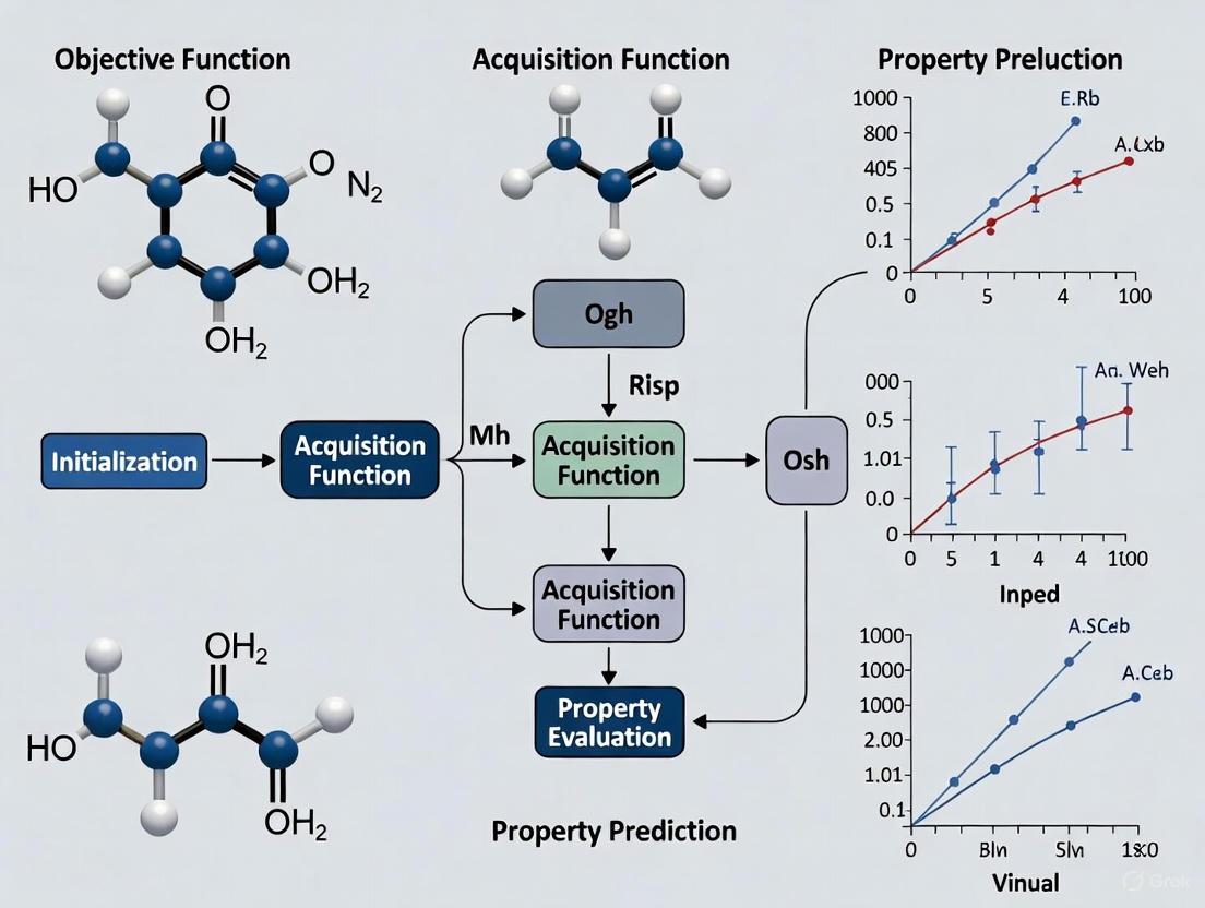
Visualizing the Bayesian Optimization Workflow
The following diagram illustrates the complete Bayesian optimization cycle as applied to molecular property prediction:
Surrogate Models in Bayesian Optimization
Gaussian Process Fundamentals
Gaussian processes (GPs) serve as the predominant surrogate model in Bayesian optimization due to their flexibility, analytical tractability, and native uncertainty quantification [8] [9]. A GP defines a distribution over functions, completely specified by a mean function ( \mu(m) ) and covariance kernel ( k(m, m') ):
[ f(m) \sim \mathcal{GP}(\mu(m), k(m, m')) ]
Given a dataset ( \mathcal{D} = {(mi, yi)}{i=1}^n ) with ( yi = F(mi) + \varepsiloni ) and ( \varepsiloni \sim \mathcal{N}(0, \lambdai) ), the posterior predictive distribution at a new point ( m ) is Gaussian with closed-form expressions for mean and variance [8]:
[ \mathbb{E}[f(m)|\mathcal{D}] = \mu(m) + \mathbf{k}n(m)^\top (\mathbf{K}n + \mathbf{\Lambda}n)^{-1} (\mathbf{y}n - \mathbf{u}n) ] [ \mathbb{V}[f(m)|\mathcal{D}] = k(m, m) - \mathbf{k}n(m)^\top (\mathbf{K}n + \mathbf{\Lambda}n)^{-1} \mathbf{k}_n(m) ]
where ( \mathbf{k}n(m) = [k(m, m1), \ldots, k(m, mn)] ), ( \mathbf{K}n ) is the covariance matrix between training points, ( \mathbf{y}n ) is the vector of observed values, ( \mathbf{u}n ) is the vector of mean values at training points, and ( \mathbf{\Lambda}_n ) is a diagonal matrix of measurement noise variances [8].
Advanced Surrogate Modeling Techniques
Table 1: Comparison of Gaussian Process Surrogate Models for Molecular Optimization
| Model Type | Key Features | Molecular Applications | Advantages | Limitations |
|---|---|---|---|---|
| Conventional GP (cGP) | Standard kernel functions (RBF, Matern) | Single-property optimization [10] | Mathematical rigor, uncertainty quantification [10] | Cannot capture property correlations [10] |
| Multi-Task GP (MTGP) | Shared kernel across related tasks | Correlated material properties [10] | Leverages correlations, improves data efficiency [10] | Complex kernel design [10] |
| Deep GP (DGP) | Hierarchical composition of GPs | Complex, non-linear property relationships [10] | Captures complex patterns [10] | Computationally intensive [10] |
| Sparse GP (SAAS) | Sparsity-inducing priors for high dimensions | Molecular descriptor libraries [8] | Automatic relevance determination, handles 100+ descriptors [8] | Requires Bayesian inference [8] |
Molecular Representations for Surrogate Modeling
The choice of molecular representation critically impacts BO performance. Common featurization approaches include:
- Descriptor-based feature vectors: Computed physicochemical properties (void fraction, pore diameters, surface area) that provide interpretable representations [11]
- Fingerprints: Binary vectors encoding molecular substructures [8]
- Learned embeddings: Neural network-generated representations via pretrained transformers (e.g., BERT) on large molecular databases [6]
The MolDAIS framework demonstrates how adaptive subspace identification within large descriptor libraries enables effective optimization in 100+ dimensional spaces using sparsity-inducing techniques [8].
Acquisition Functions: Strategic Guidance of Experiments
Taxonomy of Acquisition Functions
Acquisition functions formalize the trade-off between exploration (sampling uncertain regions) and exploitation (sampling promising regions) by quantifying the expected utility of evaluating a candidate point. The following diagram illustrates the decision logic for common acquisition functions:
Quantitative Comparison of Acquisition Strategies
Table 2: Performance Comparison of Acquisition Functions in Molecular Optimization
| Acquisition Function | Mathematical Formulation | Optimization Type | Molecular Application Results | Computational Complexity |
|---|---|---|---|---|
| Expected Improvement (EI) | ( \mathbb{E}[\max(f(m) - f(m^+), 0)] ) | Single-objective | Identifies optimal MOFs for methane storage [11] | Moderate |
| Probability of Improvement (PI) | ( P(f(m) \geq f(m^+) + \xi) ) | Single-objective | Selects informative MOFs for adsorption modeling [11] | Low |
| Upper Confidence Bound (UCB) | ( \mu(m) + \kappa\sigma(m) ) | Single-objective | Molecular property optimization with trade-off parameter κ [8] | Low |
| BALD | ( \mathbb{I}[\theta, y \mid m, \mathcal{D}] ) | Active Learning | Toxic compound identification with 50% fewer iterations [6] | High (requires posterior) |
| GP Standard Deviation | ( \sigma(m) ) | Pure Exploration | Uncertainty sampling for broad coverage [11] | Low |
Integrated Experimental Protocols
Protocol 1: Molecular Property Optimization with Adaptive Descriptors
Objective: Identify molecules with optimal target properties from large chemical libraries using the MolDAIS framework [8].
Materials and Reagents:
- Chemical Library: >100,000 candidate molecules (e.g., ZINC database, CoRE MOFs [11])
- Descriptor Software: RDKit, Dragon for molecular descriptor calculation
- BO Framework: Custom implementation with SAAS prior or adaptive screening variants
Procedure:
- Featurization Phase:
- Compute comprehensive descriptor library (150+ descriptors) for all molecules in search space
- Standardize descriptors to zero mean and unit variance
Initial Experimental Design:
- Select 5-10 initial points via Latin hypercube sampling across descriptor space
- Evaluate initial molecules via simulation or experiment to create training set ( \mathcal{D}_0 )
BO Iteration Loop:
- Train GP surrogate with SAAS prior on current data ( \mathcal{D}_t )
- Optimize acquisition function (EI recommended) to select next candidate ( m_{t+1} )
- Evaluate property of ( m_{t+1} ) via experiment/simulation
- Update dataset: ( \mathcal{D}{t+1} = \mathcal{D}t \cup {(m{t+1}, y{t+1})} )
- Check convergence (minimum improvement threshold or evaluation budget)
Termination:
- Return best-performing molecule after 50-100 evaluations
- Analyze identified descriptor subspace for interpretability
Validation: Benchmark against random search and conventional BO on public molecular datasets (Tox21, ClinTox [6]). Expected performance: Identifies near-optimal candidates with 50% fewer evaluations than conventional approaches [8].
Protocol 2: Multi-Objective Materials Discovery with Hierarchical GPs
Objective: Discover high-entropy alloy compositions optimizing multiple correlated properties (e.g., low thermal expansion coefficient and high bulk modulus) [10].
Materials:
- Search Space: FeCrNiCoCu high-entropy alloy composition space
- Characterization: High-throughput atomistic simulations for property evaluation
- Modeling Framework: MTGP or DGP with advanced kernel structures
Procedure:
- Multi-Objective Framework Setup:
- Define property targets and constraints (e.g., CTE < target, BM > threshold)
- Formulate weighted objective function or Pareto optimization scheme
Surrogate Model Configuration:
- Implement MTGP with coregionalization kernel to capture property correlations
- Alternative: DGP with 2-3 hidden layers for hierarchical representation learning
Parallel BO Execution:
- Use batch acquisition function (e.g., q-EI) for parallel evaluation of 3-5 compositions
- Evaluate candidate compositions via atomistic simulations
- Update surrogate model with all new data points
Iteration and Analysis:
- Continue for 20-30 iterations (100-150 total evaluations)
- Analyze predicted property correlations and composition-property relationships
- Validate top candidates with additional characterization
Validation: Compare against cGP-BO on FeCrNiCoCu HEA system. Expected performance: MTGP-BO and DGP-BO achieve 30-50% faster convergence by exploiting property correlations [10].
Table 3: Essential Research Reagents and Computational Tools for Molecular BO
| Category | Specific Tools/Resources | Function | Application Context |
|---|---|---|---|
| Molecular Representations | RDKit, Dragon descriptors, MolBERT embeddings [6] | Convert molecular structures to feature vectors | Create input representations for surrogate models |
| Surrogate Modeling | GPflow, GPyTorch, STAN (for SAAS) | Build probabilistic models of molecular property functions | Implement cGP, MTGP, DGP, or sparse GP models |
| Acquisition Optimization | BoTorch, Scipy optimize | Maximize acquisition functions to select candidates | Implement EI, UCB, PI, and information-theoretic functions |
| Experimental Platforms | High-throughput simulation (GCMC [11]), automated synthesis robots | Evaluate candidate molecules/properties | Generate training data for BO cycles |
| Benchmark Datasets | Tox21 [6], ClinTox [6], CoRE MOFs [11] | Validate BO performance | Compare algorithms on public molecular property data |
Bayesian optimization represents a paradigm shift in data-efficient molecular discovery, enabling researchers to navigate vast chemical spaces with minimal experimental resources. The interplay between surrogate models and acquisition functions creates a powerful framework for iterative experimental design: surrogate models provide probabilistic estimates of molecular properties, while acquisition functions strategically guide experimentation toward maximally informative candidates. For molecular scientists, mastering this cycle enables accelerated discovery of novel materials, pharmaceuticals, and functional compounds while dramatically reducing experimental costs. The protocols and analyses presented here provide both theoretical foundation and practical methodologies for implementing BO in diverse molecular optimization scenarios, from single-property drug candidate identification to multi-objective materials design.
Bayesian optimization (BO) has emerged as a powerful paradigm for the sample-efficient optimization of expensive black-box functions, making it particularly well-suited for molecular property prediction and design in drug discovery. The core challenge in this field lies in navigating the vast, high-dimensional chemical space with a limited budget for costly simulations or wet-lab experiments. This document provides detailed application notes and protocols for implementing the three key components of a Bayesian optimization framework—Gaussian Processes (GPs), Random Forests (RFs), and the Expected Improvement (EI) acquisition function—specifically within the context of molecular property optimization (MPO). We frame this within a broader thesis on advancing Bayesian optimization for drug design, providing researchers and scientists with practical, experimentally validated methodologies.
Key Components: Technical Specifications and Performance
The following table summarizes the core technical aspects and recent performance findings for each key component in the context of molecular property research.
Table 1: Key Components for Bayesian Molecular Optimization
| Component | Key Function | Recent Findings & Performance | Theoretical Advances |
|---|---|---|---|
| Gaussian Process (GP) | Probabilistic surrogate model for the black-box molecular property function. | Using Matérn kernels enables standard GP-BO to achieve top-tier results in high-dimensional settings, often surpassing specialized methods [12]. | A robust initialization strategy mitigates gradient vanishing in SE kernels, making them competitive [12]. |
| Expected Improvement (EI) | Acquisition function that balances exploration and exploitation by quantifying potential improvement. | GP-EI with BPMI/BSPMI incumbents achieves sublinear cumulative regret (no-regret) for SE and Matérn kernels [13] [14]. | EI has been reinterpreted as a variational approximation of information-theoretic acquisition functions, leading to novel hybrids like VES-Gamma [15]. |
| Random Forest (RF) | Non-parametric ensemble model that can be used as a surrogate or for hyperparameter tuning. | A Bayesian-optimized RF model achieved R² values of 0.915 (training) and 0.965 (independent test) in predicting loess collapsibility, demonstrating high reliability [16]. | Integrated with BO for hyperparameter optimization, RF models show marked improvements in optimizing search efficiency, especially with sparse target data [16] [17]. |
Integrated Workflow for Molecular Property Optimization
The synergy between GPs, EI, and RFs enables a powerful, data-efficient workflow for molecular discovery. The following diagram illustrates the typical closed-loop Bayesian optimization process, adapted for molecular property prediction.
Detailed Experimental Protocols
Protocol 1: High-Dimensional Molecular Optimization with Gaussian Processes
This protocol leverages recent findings on the robustness of standard GPs with Matérn kernels for high-dimensional Bayesian optimization [12] [8].
- Objective: To identify a molecule with an optimal target property from a large, high-dimensional chemical library using a Gaussian Process surrogate model.
- Materials & Reagents:
- Molecular Library: A discrete set of >100,000 molecules (e.g., from ZINC or Enamine databases).
- Featurization: A comprehensive library of molecular descriptors (e.g., RDKit descriptors, MOE descriptors) or a pretrained molecular transformer model (e.g., MolBERT) for generating fixed representations [6] [8].
- Software: A BO software package supporting GPs and SAAS priors (e.g., BoTorch, GPyOpt).
- Step-by-Step Procedure:
- Featurization: Encode all molecules in the library into a numerical feature vector using the chosen descriptor set or pretrained model.
- Initial Design: Randomly select a small initial set of molecules (e.g., 10-20) from the library, ensuring diversity (e.g., via scaffold splitting) [6].
- Data Collection: Obtain the target property value (e.g., binding affinity, solubility) for each molecule in the initial set via simulation or experiment.
- Model Training: Initialize a Gaussian Process surrogate model with a Matérn kernel (e.g., ν=5/2). For very high-dimensional descriptor spaces (>100), employ the SAAS (Sparse Axis-Aligned Subspace) prior to promote sparsity and adaptively identify relevant features [8].
- Candidate Selection: Using the trained GP, compute the Expected Improvement (EI) acquisition function across the entire molecular library. Select the molecule that maximizes EI.
- Iterative Loop: Evaluate the selected molecule, update the training dataset, and retrain the GP model. Repeat steps 5-6 until the evaluation budget (typically <100 evaluations) is exhausted or a performance plateau is reached.
- Validation: The success of the optimization is measured by the discovered molecule's property value and the rate of convergence. Performance is benchmarked against other MPO methods (e.g., graph-based BO, SMILES-based BO) on the same task [8].
Protocol 2: Tuning Predictive Models with Bayesian-Optimized Random Forests
This protocol uses the EI acquisition function to tune the hyperparameters of a Random Forest model, which can then be used for fast, interpretable property prediction [16].
- Objective: To optimize the hyperparameters of a Random Forest regressor for accurately predicting a molecular property, minimizing the root mean squared error (RMSE) on a validation set.
- Materials & Reagents:
- Dataset: A labeled molecular dataset (e.g., Tox21, ClinTox) split into training, validation, and test sets using scaffold splitting [6].
- Software: A machine learning library (e.g., scikit-learn) and a Bayesian optimization package (e.g., scikit-optimize).
- Step-by-Step Procedure:
- Define Search Space: Define the Bayesian optimization search space for key RF hyperparameters: number of trees (
n_estimators: 50-500), maximum tree depth (max_depth: 3-20), and minimum samples per leaf (min_samples_leaf: 1-10). - Set Objective Function: The objective function for the BO is the RMSE achieved by the RF model on the held-out validation set.
- Initialization: Start with a small number (e.g., 10) of random points in the hyperparameter space.
- BO Loop: For a fixed number of iterations (e.g., 50):
- The GP surrogate models the relationship between hyperparameters and validation RMSE.
- The EI acquisition function identifies the most promising hyperparameter set to evaluate next.
- The RF model is trained with the proposed hyperparameters and evaluated on the validation set.
- The result is used to update the GP surrogate.
- Final Model: Train a final RF model using the best-found hyperparameters on the combined training and validation set, and report its performance on the independent test set.
- Define Search Space: Define the Bayesian optimization search space for key RF hyperparameters: number of trees (
- Validation: The model's performance is quantified using R² and RMSE on the independent test set. A successfully tuned model should achieve high R² values, as demonstrated by the result of 0.965 reported in a recent study [16].
Protocol 3: No-Regret Molecular Design with Expected Improvement
This protocol focuses on the critical implementation details of the EI acquisition function to ensure robust and theoretically sound performance in noisy experimental settings [13] [14].
- Objective: To implement a no-regret Bayesian optimization algorithm for molecular design using the Expected Improvement acquisition function with a theoretically robust incumbent strategy.
- Materials & Reagents:
- Software: A Bayesian optimization library that allows custom incumbent selection (e.g., BoTorch).
- Setup: A trained GP surrogate model and a pool of unlabeled, featurized molecules.
- Step-by-Step Procedure:
- Incumbent Selection: Choose an incumbent strategy based on the noise level of your experimental data.
- For low-noise settings: Use the Best Posterior Mean Incumbent (BPMI), which finds the molecule with the best predicted mean across the entire domain. This offers the strongest theoretical guarantees but is computationally more expensive [14].
- For high-noise or large-scale settings: Use the Best Sampled Posterior Mean Incumbent (BSPMI), which selects the best mean from the set of already-sampled molecules. This is computationally cheaper and maintains no-regret properties [13] [14].
- Avoid the Best Observation Incumbent (BOI) in high-noise settings, as it can be brittle and lead to poor cumulative regret [14].
- EI Calculation: Calculate the Expected Improvement for each molecule in the pool. The standard EI formula is:
EI(x) = E[max(0, f(x) - f_incumbent)], wheref_incumbentis the value from the chosen incumbent strategy. - Molecule Selection: Select the molecule with the maximum EI value for the next experiment.
- Iteration: Update the GP model with the new data and repeat the process.
- Incumbent Selection: Choose an incumbent strategy based on the noise level of your experimental data.
- Validation: The algorithm's performance is tracked via cumulative regret. A no-regret algorithm will show a sublinear growth in cumulative regret, meaning the average regret
R_T/Tapproaches zero as the number of iterationsTincreases [13] [14].
The Scientist's Toolkit: Essential Research Reagents & Materials
Table 2: Key Research Reagents and Computational Tools for Bayesian Molecular Optimization
| Item Name | Function / Role | Specifications / Examples |
|---|---|---|
| Molecular Descriptor Libraries | Provides a fixed, chemically meaningful numerical representation of molecules for the surrogate model. | RDKit descriptors, Dragon descriptors; Used in frameworks like MolDAIS for adaptive feature selection [8]. |
| Pretrained Molecular Transformer (MolBERT) | Provides high-quality, context-aware molecular representations that disentangle feature learning from uncertainty estimation, drastically improving data efficiency [6]. | A BERT model pretrained on 1.26 million compounds; integrated into the AL pipeline to structure the embedding space [6]. |
| Sparse Axis-Aligned Subspace (SAAS) Prior | A Bayesian prior applied to the GP surrogate model that promotes sparsity, allowing it to ignore irrelevant descriptors and focus on task-relevant features in high-dimensional spaces [8]. | Key component of the MolDAIS framework; enables efficient optimization in descriptor libraries with thousands of features [8]. |
| Benchmark Molecular Datasets | Standardized datasets for training, validating, and benchmarking model performance in fair and comparable ways. | Tox21 (12 toxicity pathways), ClinTox (FDA-approved vs. failed drugs) [6]. |
| Scaffold Splitting Algorithm | A data splitting method that partitions molecules based on core structural scaffolds, ensuring that test sets contain novel chemotypes not seen during training. This tests a model's true generalization ability [6]. | Bemis-Murcko scaffold representation; crucial for evaluating real-world utility in drug discovery [6]. |
{# Abstract}
This application note addresses the central challenge of balancing exploration and exploitation within Bayesian optimization (BO) frameworks for molecular property prediction and materials discovery. Designed for researchers and drug development professionals, it details practical protocols and frameworks that dynamically manage this trade-off, enabling efficient navigation of high-dimensional chemical spaces with minimal experimental resource expenditure.
The application of Bayesian optimization (BO) in molecular sciences represents a paradigm shift in the acceleration of drug design and materials discovery. BO is a sample-efficient, sequential strategy for the global optimization of expensive-to-evaluate "black-box" functions, a category that includes complex laboratory experiments and detailed molecular simulations [9]. Its core strength lies in a principled balance between exploration (probing regions of high uncertainty in the search space) and exploitation (refining knowledge in areas known to yield good results) [9].
However, the vastness and high dimensionality of molecular search spaces pose a critical challenge. The effectiveness of BO is heavily dependent on the numerical representation, or featurization, of molecules and materials [4] [8]. High-dimensional representations can cripple BO performance due to the "curse of dimensionality," while an incomplete representation that misses key features can bias the search irrevocably [4]. This note presents and protocols advanced frameworks that integrate adaptive feature selection and sophisticated surrogate models to overcome this challenge, ensuring robust and data-efficient optimization.
Core Principles and Adaptive Frameworks
The power of Bayesian optimization stems from three core components: Bayesian inference for updating beliefs with new evidence, a Gaussian Process (GP) as a probabilistic surrogate model of the objective function, and an acquisition function to manage the exploration-exploitation trade-off [9].
Key Components of Bayesian Optimization
- Gaussian Process Surrogate Model: A GP defines a distribution over functions, providing for any input (e.g., a molecular descriptor vector) both a prediction (mean) and a measure of uncertainty (variance) [9] [10]. This uncertainty quantification is essential for guiding the search.
- Acquisition Functions: This function uses the GP's output to score the utility of evaluating any candidate point. Common functions include:
- Expected Improvement (EI): Selects points offering the highest expected improvement over the current best observation [4] [8].
- Upper Confidence Bound (UCB): Selects points by maximizing an upper confidence bound on the prediction, with a tunable parameter to balance exploration and exploitation [4] [9].
- Probability of Improvement (PI) and Bayesian Active Learning by Disagreement (BALD) are other examples used in different contexts [9] [6].
Advanced Frameworks for Adaptive Representation
Traditional BO uses a fixed molecular representation, which can be suboptimal. Recent frameworks address this by dynamically adapting the feature set during optimization.
- Feature Adaptive Bayesian Optimization (FABO): This framework integrates feature selection directly into the BO cycle. It starts with a complete, high-dimensional feature set and, at each cycle, uses methods like Maximum Relevancy Minimum Redundancy (mRMR) or Spearman ranking to identify and retain the most informative features for the specific task. This leads to a compact, task-relevant representation that enhances BO efficiency without requiring prior expert knowledge [4].
- Molecular Descriptors with Actively Identified Subspaces (MolDAIS): MolDAIS leverages the sparse axis-aligned subspace (SAAS) prior to induce sparsity in the feature space. It constructs parsimonious GP models that actively identify and focus on a low-dimensional, task-relevant subspace from a large library of molecular descriptors as new data is acquired [8].
Quantitative Performance Comparison
The following tables summarize the performance of adaptive BO methods against baselines in various molecular and materials optimization tasks.
Table 1: Performance in Molecular and Materials Discovery Tasks
| Framework | Optimization Task | Search Space Size | Performance vs. Baseline | Key Metric |
|---|---|---|---|---|
| FABO [4] | MOF for CO₂ uptake & band gap | ~8,500 - 9,500 materials | Outperformed random search and fixed-representation BO | Accelerated identification of top performers |
| MolDAIS [8] | Molecular Property Optimization | >100,000 molecules | Outperformed state-of-the-art methods (graphs, SMILES, embeddings) | Identified near-optimal candidates in <100 evaluations |
| BioKernel [9] | Limonene production in E. coli | 4-dimensional input space | 78% fewer evaluations than grid search | Converged to optimum in 18 vs. 83 points |
| Pretrained BERT + BALD [6] | Toxic compound identification (Tox21, ClinTox) | ~1,484 - 8,000 compounds | 50% fewer iterations than conventional active learning | Equivalent identification accuracy |
Table 2: Comparison of Feature Selection and Surrogate Model Methods
| Method | Feature Selection / Model Approach | Key Advantage | Best Suited For |
|---|---|---|---|
| mRMR [4] | Selects features balancing relevance to target and redundancy among themselves | Creates a compact, non-redundant feature set | General-purpose optimization with a full feature pool |
| Spearman Ranking [4] | Univariate ranking based on monotonic correlation with target | Computational efficiency and simplicity | Quick initialization or low-dimensional targets |
| SAAS Prior [8] | Fully Bayesian GP with sparsity-inducing prior | Automatically identifies sparse, relevant subspaces | High-dimensional descriptor libraries with inherent sparsity |
| Mutual Information (MI) / MIC [8] | Screening variants for scalable subspace selection | Runtime efficiency with retained interpretability | Large feature sets where full SAAS is prohibitive |
| Multi-task GP (MTGP) [10] | Models correlations between distinct material properties | Leverages information from correlated objectives | Multi-objective optimization with related properties |
Detailed Experimental Protocols
Protocol 1: Implementing FABO for MOF Discovery
Application: Discovering metal-organic frameworks (MOFs) with optimal properties like gas uptake or electronic band gap [4].
Workflow Overview:
FABO Cycle for MOF Discovery
Step-by-Step Procedure:
Problem Formulation:
- Objective: Define the target property (e.g., CO₂ uptake at 16 bar, electronic band gap).
- Search Space: Define the database of MOF candidates (e.g., QMOF, CoRE-2019) [4].
Initialization and Featurization:
- Feature Pool: Represent each MOF with a comprehensive set of features, including:
- Initial Sampling: Select a small initial set of MOFs (e.g., via random sampling or Latin Hypercube) for labeling.
Closed-Loop FABO Cycle:
- Data Labeling: Obtain the target property value for the selected MOF via simulation or experiment.
- Adaptive Feature Selection:
- Using all data acquired so far, apply a feature selection method.
- For mRMR: Iteratively select features that maximize relevance (F-statistic with target) and minimize redundancy (average correlation with already-selected features) [4].
- For Spearman: Rank all features by the absolute value of their Spearman rank correlation coefficient with the target and select the top k.
- Surrogate Model Update: Train a Gaussian Process model using only the currently selected, adapted feature set.
- Candidate Selection:
- Using an acquisition function (e.g., EI, UCB) on the updated GP model, evaluate all MOFs in the database.
- Select the MOF with the highest acquisition function value as the next candidate for labeling.
Termination: The cycle repeats until a convergence criterion is met (e.g., a performance target is achieved, a maximum number of iterations is reached, or the improvement between cycles becomes negligible).
Protocol 2: Molecular Optimization with MolDAIS
Application: Single- or multi-objective optimization of molecular properties from large chemical libraries [8].
Workflow Overview:
MolDAIS Framework for Molecular Optimization
Step-by-Step Procedure:
Problem Formulation:
- Define the molecular property(s) to optimize.
- Define the discrete molecular search space (e.g., a chemical library with over 100,000 molecules) [8].
Featurization:
- Compute a comprehensive library of molecular descriptors for every molecule in the search space. This can include simple atom counts, topological indices, quantum-chemical descriptors, etc. [8].
MolDAIS Initialization:
- Impose a SAAS prior on the GP surrogate model. This prior assumes that only a sparse subset of the descriptor dimensions is actively relevant to the property [8].
- Begin with a small initial dataset.
Closed-Loop Optimization:
- Acquire Data: Obtain the property value for the proposed molecule.
- Update Surrogate Model: Perform Bayesian inference (e.g., using Hamiltonian Monte Carlo) to update the GP model. This process automatically infers the "active" descriptors (those with non-zero length scales) and shrinks the influence of irrelevant ones.
- Propose Next Candidate: Optimize the acquisition function (e.g., EI) over the entire molecular search space using the updated model to find the most promising molecule to evaluate next.
Termination: Cycle continues until the evaluation budget is exhausted or convergence is achieved.
The Scientist's Toolkit: Research Reagent Solutions
Table 3: Essential Computational Tools and Datasets
| Item | Function / Description | Example Use Case |
|---|---|---|
| Gaussian Process (GP) Regressor | Core surrogate model for BO; provides predictions with uncertainty estimates. | Modeling the relationship between molecular features and a target property [4] [10]. |
| Molecular Descriptor Libraries | Precomputed sets of numerical features (e.g., RACs, topological indices) representing molecular structure. | Featurizing molecules for input into the BO model [4] [8]. |
| mRMR Algorithm | Feature selection method to maximize relevance and minimize redundancy. | Creating a compact, informative feature set within FABO [4]. |
| SAAS Prior | A sparsity-inducing prior for GPs that promotes the use of only a subset of input features. | Enabling automatic feature selection in the MolDAIS framework [8]. |
| QMOF Database | A database of over 8,000 MOFs with computed electronic properties from DFT. | Search space for MOF band gap or electronic property optimization [4]. |
| CoRE MOF Database | A database of thousands of MOFs with gas adsorption data. | Search space for optimizing MOFs for gas storage or separation [4]. |
| Tox21/ClinTox Datasets | Publicly available datasets with toxicology data for thousands of compounds. | Benchmarking optimization and active learning for drug safety [6]. |
Advanced BO Strategies and Real-World Applications in Molecular Design
Molecular property optimization (MPO) is a central challenge in fields ranging from drug discovery to materials science. The effectiveness of these optimization campaigns critically depends on the molecular representation used. Traditional fixed representations, such as fingerprints and descriptors, often struggle in high-dimensional, low-data regimes. This article details the application of two advanced Bayesian optimization (BO) frameworks—MolDAIS (Molecular Descriptors with Actively Identified Subspaces) and FABO (Feature Adaptive Bayesian Optimization)—that overcome these limitations by dynamically adapting their molecular representations to identify optimal candidates with exceptional sample efficiency [8] [18].
While both MolDAIS and FABO share the core principle of adaptive representation within a Bayesian optimization context, they are distinct frameworks with different methodological approaches and origins.
MolDAIS: Molecular Descriptors with Actively Identified Subspaces
MolDAIS is a flexible BO framework designed for data-efficient chemical design. Its core innovation lies in adaptively identifying a sparse, task-relevant subspace from a large, precomputed library of molecular descriptors during the optimization process. This approach avoids the high dimensionality and potential irrelevance of fixed representations by focusing the surrogate model on a minimal set of informative features [19] [8].
FABO: Feature Adaptive Bayesian Optimization
FABO is a framework that integrates feature selection directly into the Bayesian optimization process. It uses Gaussian processes to dynamically adapt material representations throughout the optimization cycles, allowing it to automatically identify molecular representations that align with human chemical intuition for known tasks and discover effective representations for novel tasks where prior knowledge is unavailable [18].
Comparative Analysis
Table: Framework Comparison: MolDAIS vs. FABO
| Feature | MolDAIS | FABO |
|---|---|---|
| Core Adaptation Mechanism | Active identification of sparse subspaces from descriptor libraries [8] | Integrated feature selection within the BO process [18] |
| Primary Representation | Precomputed molecular descriptor libraries | Molecular features adapted via Gaussian processes |
| Key Innovation | Sparsity-inducing priors (SAAS) & screening variants (MI, MIC) for scalability [8] | Dynamic adaptation of representations across BO cycles [18] |
| Reported Performance | Identifies near-optimal molecules from >100k library in <100 evaluations [8] | Outperforms random search and fixed-representation baselines [18] |
| Interpretability | High; provides a compact set of relevant molecular descriptors [8] | High; identifies representations aligned with chemical intuition [18] |
Experimental Protocols and Performance Benchmarks
This section provides detailed methodologies for implementing and evaluating the MolDAIS and FABO frameworks, based on published results.
MolDAIS Protocol: Single-Objective Molecular Optimization
The following protocol is adapted from the MolDAIS quick start example and methodological paper [19] [8].
1. Problem Initialization
- Define Search Space: Compile a list of candidate molecules as SMILES strings.
- Compute Target Properties: Obtain or calculate the target property values (e.g., logP) for a labeled subset, formatted as a PyTorch tensor.
- Initialize Problem Object: Create a
MolDAIS.Problemobject, specifying the SMILES list, target values, and an experiment name. Executeproblem.compute_descriptors()to featurize the molecules.
2. Optimizer Configuration
Configure the OptimizerParameters object. Critical parameters include:
sparsity_method: Feature selection method ('MI' for Mutual Information or 'MIC').acq_fun: Acquisition function ('EI' for Expected Improvement).num_sparsity_feats: Number of features to select (e.g., 10).total_sample_budget: Total function evaluations (e.g., 7).initialization_budget: Initial random samples for model warm-up (e.g., 2).
3. Execution and Analysis
- Instantiate the
MolDAISclass with the problem and parameters. - Run the optimization via
mol_dais.configuration.optimize(). - Access results:
mol_dais.results.best_moleculesandmol_dais.results.best_values. - Visualize convergence:
mol_dais.configuration.plot_convergence().
4. Performance Benchmark In rigorous testing, MolDAIS demonstrated the ability to identify high-performing molecules from large chemical libraries. The table below summarizes its data-efficient performance across various tasks [8].
Table: MolDAIS Performance Benchmarks
| Optimization Task | Search Space Size | Evaluation Budget | Key Performance Outcome |
|---|---|---|---|
| Single-objective MPO | >100,000 molecules | <100 evaluations | Identified near-optimal candidates [8] |
| Multi-objective MPO | Large-scale libraries | <100 evaluations | Consistently outperformed state-of-the-art baselines [8] |
| Organic Electrode Discovery | Real-world experimental space | Low budget (specific n not stated) | Found candidates matching/surpassing state-of-the-art at lower cost [20] |
FABO Protocol: Adaptive Representation in BO
The general workflow for FABO, which integrates feature selection with the BO loop, can be summarized as follows [18]:
1. Initialization
- Start with a full set of molecular features or descriptors.
- Define the black-box objective function to be optimized.
2. Iterative Optimization Loop
- Surrogate Modeling: Train a Gaussian process model on the currently collected data, using the dynamically adapted feature subset.
- Feature Selection: The model updates its hypothesis about the relevant feature subspace based on the accumulated data.
- Acquisition and Evaluation: Use an acquisition function to select the next promising molecule for evaluation based on the adapted model.
- Data Update: Augment the dataset with the new evaluation result.
3. Output After the evaluation budget is exhausted, the framework returns the best-performing molecule(s) found, along with the final adapted molecular representation.
The Scientist's Toolkit: Essential Research Reagents
The following table catalogs the key computational tools and components required to implement adaptive representation frameworks like MolDAIS and FABO.
Table: Key Research Reagent Solutions for Adaptive Molecular Optimization
| Tool/Component | Function | Example/Note |
|---|---|---|
| Molecular Descriptor Libraries | Provides a comprehensive set of featurizations for molecules, serving as the initial input for frameworks like MolDAIS. | RDKit 2D descriptors (200 features), Morgan Fingerprints (ECFP) [21] [8] |
| Sparsity-Inducing Surrogate Models | The core model that actively identifies a sparse, relevant subset of features from the full library during optimization. | Gaussian Process with SAAS (Sparse Axis-Aligned Subspace) prior [8] |
| Bayesian Optimization Backbone | Provides the algorithmic engine for sample-efficient, sequential experimental design. | Bayesian Optimization loop with acquisition functions like Expected Improvement (EI) [19] [8] |
| Domain-Specific Objective Function | The expensive black-box function representing the molecular property to be optimized. | Can be a high-fidelity simulation, a machine learning model, or an experimental measurement [8] [20] |
Workflow Visualization
The following diagram illustrates the core adaptive loop of the MolDAIS framework, from molecular search space to iterative subspace refinement.
Diagram: The MolDAIS Adaptive Bayesian Optimization Loop
MolDAIS and FABO represent a significant shift from static to adaptive molecular representations in Bayesian optimization. By actively learning which features matter most for a specific task, these frameworks achieve remarkable sample efficiency, making them exceptionally well-suited for real-world applications where data is scarce and costly to acquire. Their ability to provide interpretable insights into the key molecular descriptors driving property optimization further enhances their utility for researchers and drug development professionals aiming to accelerate the discovery of novel molecules and materials.
Leveraging Multi-Fidelity Bayesian Optimization for Experimental Funnels
Multi-fidelity Bayesian Optimization (MFBO) is an advanced machine learning framework that accelerates scientific discovery by intelligently integrating data sources of varying cost and accuracy. In the context of molecular property prediction and materials research, it addresses a critical challenge: experimental resources are finite and high-fidelity measurements (e.g., precise biological activity assays) are often expensive and time-consuming. MFBO leverages cheaper, lower-fidelity approximations (e.g., computational simulations or rapid preliminary screens) to guide the optimization process more efficiently than using high-fidelity data alone [22]. By building a probabilistic model that understands the relationships between different information sources, MFBO strategically decides which experiment to perform and at what fidelity, maximizing learning while minimizing total cost [22] [23]. This document provides detailed application notes and protocols for implementing MFBO within experimental funnels for molecular property optimization, framed within a broader thesis on Bayesian optimization for molecular research.
Core Concepts and Quantitative Foundations
Bayesian Optimization Refresher
Bayesian Optimization (BO) is a sample-efficient strategy for optimizing expensive-to-evaluate black-box functions [24]. It operates through two key components:
- Surrogate Model: Typically a Gaussian Process (GP), which provides a probabilistic approximation of the objective function, giving a mean prediction and uncertainty estimate at any point in the search space [24] [25].
- Acquisition Function: A policy that uses the surrogate's predictions to select the next most promising point to evaluate by balancing exploration (high uncertainty) and exploitation (high predicted value) [24]. Common acquisition functions include Expected Improvement (EI) and Upper Confidence Bound (UCB) [25].
Multi-Fidelity Extension
MFBO extends this core BO framework by incorporating multiple information sources, or fidelities. A high-fidelity (HF) source represents the expensive, accurate measurement (e.g., final experimental validation), while one or more low-fidelity (LF) sources provide cheaper, less accurate approximations (e.g., computational models or simplified experimental assays) [22]. The multi-fidelity surrogate model, often a multi-task GP, learns the correlation between these fidelities, allowing knowledge transfer from abundant LF data to inform predictions at the HF level [22].
When Does MFBO Succeed? A Quantitative Guide
The performance advantage of MFBO over single-fidelity BO (SFBO) is not guaranteed; it depends critically on the characteristics of the low-fidelity source. Systematic studies on synthetic functions (e.g., Branin, Park) have quantified the conditions for success [22].
Table 1: Impact of Low-Fidelity Source Characteristics on MFBO Performance
| Characteristic | Favorable Condition for MFBO | Unfavorable Condition for MFBO | Quantitative Impact on Performance (Δ) |
|---|---|---|---|
| Cost Ratio (ρ)(Cost of LF / Cost of HF) | Low (e.g., ρ = 0.1) | High (e.g., ρ = 0.5) | Inverse correlation; lower cost yields higher performance gain (Δ) [22] |
| Informativeness (R²)(Correlation between LF and HF) | High (e.g., R² > 0.9) | Low (e.g., R² < 0.75) | Direct correlation; higher R² yields higher performance gain (Δ) [22] |
| Combined Effect | Cheap & Informative LF | Expensive & Non-informative LF | Maximum Δ observed in favorable scenarios (e.g., 0.53); negative Δ (worse than SFBO) in unfavorable scenarios [22] |
The performance gain, Δ, is a key metric comparing the normalized performance of MFBO against SFBO, with positive values indicating an advantage for MFBO [22]. The data shows a clear gradient where progression towards cheaper and more informative LF sources provides better MFBO performance [22].
MFBO Protocol for Molecular Property Optimization
This protocol outlines the steps for employing MFBO to optimize a target molecular property (e.g., drug candidate binding affinity).
Pre-Experimental Planning
Step 1: Define Fidelity Hierarchy
- High-Fidelity (HF): Define the primary, expensive experimental endpoint. Example: IC₅₀ determination from a full, validated biochemical assay. Cost is normalized to 1.
- Low-Fidelity (LF): Identify one or more cheaper, faster proxies. Examples:
- Assign Costs: Quantify the relative cost (time, resources) of each LF source relative to HF. Example: Computational docking cost ρ = 0.01; HTS assay cost ρ = 0.1 [22].
Step 2: Characterize Fidelity Relationship
- If historical data exists, compute the correlation (e.g., R²) between the LF and HF outputs for a set of representative molecules. An R² > 0.8 suggests high informativeness [22].
- If no data exists, use domain expertise to estimate the expected correlation and proceed; the MFBO model will refine this understanding during optimization.
Step 3: Initial Experimental Design
- Using a space-filling design (e.g., Latin Hypercube Sampling), select an initial set of 5-10 molecules to be evaluated at the HF level.
- Optionally, evaluate a larger set of molecules (e.g., 50-100) at the primary LF level to seed the model with initial data [22].
Iterative MFBO Loop
The core optimization process is an iterative cycle.
Step 4: Model Initialization
- Fit a multi-fidelity Gaussian Process surrogate model to all available data. The model should use a kernel designed to capture correlations across fidelities (e.g., in BoTorch) [22].
Step 5: Candidate Suggestion via Acquisition Function
- Use a cost-aware acquisition function to select the next molecule and fidelity level to evaluate. The function balances three factors:
- Potential Improvement: Based on the surrogate model's prediction.
- Uncertainty Reduction: The value of exploring uncertain regions.
- Cost: The relative expense of the fidelity level.
- Common choices are the Multi-Fidelity Expected Improvement or Upper Confidence Bound.
Step 6: Execution and Data Incorporation
- Execute the experiment as suggested by the acquisition function (e.g., synthesize the proposed molecule and run it at the specified fidelity level).
- Add the new data point (molecule, fidelity, observed result) to the training dataset.
Step 7: Termination Check
- The loop (Steps 4-6) repeats until a stopping criterion is met, such as:
- Exhaustion of the experimental budget.
- Convergence (minimal improvement over several iterations).
- Discovery of a molecule meeting the target property threshold.
The Scientist's Toolkit: Research Reagent Solutions
Table 2: Essential Materials and Computational Tools for MFBO Implementation
| Item Name | Function/Description | Example in Molecular Context |
|---|---|---|
| High-Fidelity Assay Kit | Provides the definitive, gold-standard measurement of the target molecular property. | Validated enzyme activity assay kit for precise IC₅₀ determination. |
| Low-Fidelity Proxy Assay | Enables rapid, cheaper approximation of the property for high-throughput screening. | Fluorescence-based initial screening assay; Computational docking software. |
| Multi-Fidelity BO Software | Computational backbone for implementing the MFBO algorithm and surrogate modeling. | BoTorch (PyTorch-based) or NUBO frameworks [22] [24]. |
| Chemical Library | A diverse set of molecules (virtual or physical) representing the search space for optimization. | Commercially available scaffold library; In-house virtual compound database. |
| Automation & LIMS | Laboratory automation systems and a Laboratory Information Management System to track experiments and data. | Liquid handling robots for assay plating; Electronic lab notebook for data logging. |
Performance Benchmarking and Analysis
Expected Outcomes
When applied under favorable conditions (cheap, informative LF), MFBO significantly reduces the total cost required to find an optimal solution compared to SFBO. The following table synthesizes performance gains observed in benchmark studies.
Table 3: MFBO Performance in Benchmark Studies
| Optimization Task / Function | Key MFBO Parameters | Performance Gain (Δ) vs. SFBO | Notes |
|---|---|---|---|
| Branin (Synthetic) | LF Cost ρ=0.1, LF R²>0.9 | Δ = 0.53 (Maximum discount) | MFBO achieves lower regrets quicker by exploiting LF data [22] |
| Park (Synthetic) | LF Cost ρ=0.1, LF R²>0.9 | Δ = 0.33 (Maximum discount) | Demonstrates effectiveness in higher-dimensional spaces [22] |
| Direct Arylation (Chemical Rxn) | Not Specified | 60.7% yield (MFBO) vs 25.2% yield (BO) | Example of LLM-enhanced Reasoning BO framework [28] |
| Bioprocess Optimization | Not Specified | 36% productivity increase | Bayesian Exp. Design optimized biomass formation [29] |
Advanced Integration: LLM-Enhanced Reasoning BO
Emerging frameworks are augmenting MFBO with Large Language Models (LLMs) to address limitations like local optima convergence and lack of interpretability. The "Reasoning BO" framework uses LLMs to generate and refine scientific hypotheses, which are then used to guide the BO sampling process [28]. For instance, in a chemical reaction yield optimization task (Direct Arylation), this hybrid approach achieved a final yield of 94.39%, compared to 76.60% for Vanilla BO, by leveraging domain knowledge and real-time reasoning [28]. This points to a future where MFBO is not just data-efficient but also scientifically insightful.
Multi-fidelity Bayesian Optimization represents a paradigm shift for efficient experimental design in molecular property prediction. Its successful application hinges on the careful selection of low-fidelity sources that are both inexpensive and informative relative to the high-fidelity goal. By following the protocols outlined herein—from pre-experimental planning and fidelity characterization to the execution of the iterative MFBO loop—researchers can systematically reduce the time and cost associated with molecular discovery and optimization. Integrating these data-driven strategies into experimental funnels promises to accelerate the pace of research in drug development and materials science.
Rank-Based Bayesian Optimization (RBO) for Rough Property Landscapes
Bayesian optimization (BO) has become an indispensable tool for autonomous decision-making across diverse applications, from autonomous vehicle control to accelerated drug and materials discovery [30]. With the growing interest in self-driving laboratories, BO of chemical systems is crucial for machine learning (ML)-guided experimental planning [31]. Traditional BO typically employs a regression surrogate model to predict the distribution of unseen parts of the search space. However, for molecular selection tasks where the goal is to pick top candidates with respect to a distribution, the relative ordering of their properties may be more important than their exact values [30] [31]. This insight has led to the development of Rank-based Bayesian Optimization (RBO), which utilizes a ranking model as the surrogate instead of traditional regression approaches [31].
The fundamental shift in RBO addresses key challenges in molecular property prediction, particularly when dealing with rough structure-property landscapes and activity cliffs—situations where small changes in molecular structure correspond to large fluctuations in property values [31]. These challenging landscapes are prevalent in drug discovery, where optimal compounds are often found precisely at these activity cliffs [31]. Regression models struggle with such rough landscapes because they attempt to predict exact property values, while ranking models focus solely on relative ordering, effectively reducing the impact of sharp changes in the functional space [31].
Theoretical Foundation: RBO vs. Regression BO
Core Conceptual Differences
Rank-Based Bayesian Optimization represents a paradigm shift from conventional regression-based BO by reformulating the surrogate modeling task from value prediction to ordinal ranking. The table below summarizes the fundamental differences between these approaches:
Table 1: Fundamental Differences Between Regression BO and Rank-Based BO
| Aspect | Regression BO | Rank-Based BO (RBO) |
|---|---|---|
| Surrogate Output | Predicts exact property values | Predicts relative rankings between candidates |
| Loss Function | Mean Squared Error (MSE) | Pairwise ranking loss (e.g., marginal ranking loss) |
| Primary Focus | Accurate value estimation | Correct ordinal relationships |
| Handling Activity Cliffs | Struggles with sharp property changes | Robust to rough landscapes and outliers |
| Data Efficiency | Requires more data for accurate regression | Effective ranking even in low-data regimes |
| Uncertainty Quantification | Predictive variance on values | Uncertainty in ranking orders |
Mathematical Formulation of Ranking Loss
The ranking loss used for Learning to Rank (LTR) tasks in RBO is typically formulated as a pairwise marginal ranking loss. Unlike point-wise loss functions like MSE that map a scalar prediction and ground truth to a scalar loss value, pairwise loss functions map a pair of predictions and a pair of ground truths to a scalar loss [31]. The pairwise marginal ranking loss has the form:
[ \mathcal{L}(y1, y2, \hat{y}1, \hat{y}2) = \max\big(0, -\textrm{sign}(y1 - y2) * (\hat{y}1 - \hat{y}2) + m\big) ]
Where ((y1, y2)) is the ground truth pair, ((\hat{y}1, \hat{y}2)) is the predicted pair, and (m) is a margin parameter that allows for predicted rank overlap (typically set to (m=0) for no margin) [31]. For correctly ranked predicted pairs, the sign of the second argument will be negative and (\mathcal{L}=0). During training, the dataset is collated into ((N^2-N)/2) unique pair combinations, where (N) is the number of data points [31].
Quantitative Performance Comparison
Performance Across Chemical Datasets
Comprehensive investigations of RBO's optimization performance compared to conventional BO on various chemical datasets demonstrate similar or improved optimization performance using ranking models [31]. The following table summarizes key quantitative findings from these studies:
Table 2: Performance Comparison of RBO vs. Regression BO on Chemical Datasets
| Dataset Characteristics | Regression BO Performance | RBO Performance | Key Observations |
|---|---|---|---|
| Rough structure-property landscapes | Suboptimal due to activity cliffs | Superior - robust to roughness | RBO maintains performance where regression fails |
| Smooth property landscapes | Excellent performance | Comparable performance | Both methods perform well in smooth spaces |
| Low-data regimes | Struggles with accurate value prediction | Superior - effective ranking with limited data | Ranking ability maintained at early BO iterations |
| High-data regimes | Excellent with sufficient data | Excellent performance | Both methods converge with ample data |
| Presence of activity cliffs | Predictive accuracy reduced | Minimal performance degradation | Ranking unaffected by sharp property changes |
| Correlation with surrogate ability | Moderate correlation | High correlation | Surrogate ranking ability strongly predicts BO performance |
Performance Metrics and Statistical Significance
Studies have demonstrated that RBO consistently achieves lower objective values and exhibits greater stability across runs compared to traditional approaches [32]. Statistical tests further confirm that RBO significantly outperforms Random Search at the 1% significance level [32]. The high correlation between surrogate ranking ability and BO performance makes RBO particularly valuable for optimization campaigns where early performance is critical [31].
Experimental Protocols and Implementation
RBO Workflow Implementation
RBO Experimental Workflow: Implementation steps for Rank-Based Bayesian Optimization
Detailed Protocol Steps
Molecular Representation and Featurization
For RBO implementation, molecules must be converted into numerical representations suitable for machine learning models. Two primary approaches are recommended:
Extended-Connectivity Fingerprints (ECFP): Use Morgan fingerprints with radius 3, implemented in cheminformatics software RDKit, to create 2048-dimensional bit vectors hashed from local structures of the molecular graph [31]. The Tanimoto distance kernel is particularly effective when using Morgan fingerprint representations [31].
Graph Neural Networks (GNN): Represent molecules as graphs with atoms as nodes and bonds as edges, along with node and edge features as defined in the Open Graph Benchmark [31]. GNNs based on the ChemProp architecture with two message-passing layers operating and a final variational inference Bayesian layer to produce uncertainty estimates are particularly effective [31].
Surrogate Model Training Protocol
Ranking Model Implementation:
- Model Architecture Selection: Choose between Multi-Layer Perceptron (MLP), Bayesian Neural Network (BNN), or Graph Neural Network (GNN) architectures [31].
- Pairwise Training Data Preparation: Collate the dataset into ((N^2-N)/2) unique pair combinations for training [31].
- Loss Function Implementation: Implement the pairwise marginal ranking loss with margin parameter (m=0) [31].
- Probabilistic Output: For Bayesian models, include regularization via KL divergence over weight distributions of variational layers [31].
- Model Training: Train until convergence with appropriate validation on ranking metrics.
Comparative Regression Model Implementation:
- Model Architecture: Use the same base architecture as ranking models for fair comparison.
- Loss Function: Implement Mean Squared Error (MSE) loss for regression tasks.
- Probabilistic Extensions: For Bayesian models, include appropriate uncertainty quantification methods.
Acquisition Function and Selection
- Acquisition Function Choice: Expected Improvement (EI) is commonly used, but other functions like Upper Confidence Bound (UCB) can be implemented [33].
- Candidate Selection: Choose top candidates based on acquisition function optimization for experimental evaluation.
- Batch Selection: For parallel experimentation, select multiple candidates using appropriate batch selection strategies.
Evaluation Metrics and Validation
Implement comprehensive evaluation strategies including:
- Ranking Performance Metrics: Kendall's Tau, Spearman's correlation between predicted and true rankings.
- Optimization Efficiency: Number of iterations to reach target performance, best value found over iterations.
- Statistical Validation: Multiple runs with different random seeds to ensure result robustness.
The Scientist's Toolkit: Research Reagent Solutions
Table 3: Essential Research Tools and Resources for RBO Implementation
| Tool/Resource | Type | Function in RBO Research | Implementation Notes |
|---|---|---|---|
| RDKit | Cheminformatics Library | Molecular featurization via ECFP fingerprints | Open-source, provides Morgan fingerprint implementation |
| PyTorch | Deep Learning Framework | Model implementation for MLP, BNN | Enables custom ranking loss implementation |
| PyTorch Geometric | GNN Library | Graph-based molecular representation | Implements message-passing layers for molecules |
| GPyTorch/GAUCHE | Gaussian Process Library | Baseline GP regression models | Provides Tanimoto kernel for molecular similarity |
| BayesMallows | Bayesian Ranking Models | Alternative ranking model implementation | Based on Mallows model for permutations |
| RBO Code Repository | Reference Implementation | Complete RBO workflow | Available at github.com/gkwt/rbo |
Application Guidelines and Decision Framework
When to Use RBO vs. Regression BO
The decision to implement Rank-Based Bayesian Optimization should be guided by specific characteristics of the optimization problem:
Use RBO when:
- Dealing with rough structure-property landscapes with activity cliffs [31]
- Working in low-data regimes where ranking is easier than regression [31]
- The primary goal is candidate prioritization rather than exact property prediction [30]
- Facing noisy or unreliable absolute measurements but reliable comparative assessments [32]
Use Regression BO when:
- Working with smooth, well-behaved property landscapes [31]
- Exact property values are critical for downstream applications
- Sufficient data is available for accurate regression modeling
- Uncertainty quantification on absolute values is required
Implementation Considerations for Molecular Optimization
For researchers implementing RBO in molecular property prediction, several practical considerations are essential:
- Representation Choice: ECFP fingerprints work well for smaller molecules, while GNN representations may capture complex structural relationships better for larger compounds [31].
- Model Selection: BNN and GNN models provide inherent uncertainty quantification valuable for BO, while standard MLPs are simpler but lack uncertainty estimates [31].
- Computational Resources: Pairwise ranking loss requires more memory due to quadratic pair generation; implement efficient sampling for large datasets [31].
- Integration with Experimental Platforms: For self-driving laboratories, ensure RBO workflow integration with automated synthesis and characterization platforms [30].
Rank-Based Bayesian Optimization represents a significant advancement for molecular optimization tasks, particularly those characterized by rough property landscapes and activity cliffs. By focusing on relative rankings rather than exact values, RBO demonstrates enhanced robustness and performance in challenging optimization scenarios prevalent in drug discovery and materials science.
The experimental protocols and implementation guidelines provided here offer researchers a comprehensive framework for applying RBO to their molecular optimization challenges. As the field advances, future developments will likely focus on hybrid approaches combining the strengths of ranking and regression models, improved uncertainty quantification for ranking, and enhanced scalability for high-throughput experimentation environments.
Integrating Pretrained Models and Active Learning for Enhanced Sample Efficiency
The discovery of molecules with optimal functional properties is a central challenge across diverse fields such as energy storage, catalysis, and chemical sensing [8]. However, molecular property optimization (MPO) remains difficult due to the combinatorial size of chemical space and the substantial cost of acquiring property labels via simulations or wet-lab experiments [8]. Bayesian optimization (BO) offers a principled framework for sample-efficient discovery in such settings, but its effectiveness depends critically on the quality of the molecular representation used to train the underlying probabilistic surrogate model [8].
Traditional machine learning approaches for molecular property prediction often struggle in low-data regimes due to high dimensionality or poorly structured latent spaces [8] [6]. Active learning (AL) provides a promising alternative by strategically selecting informative molecules for labeling, thereby reducing experimental costs [6]. However, conventional active learning typically trains models on labeled examples alone, neglecting valuable information present in unlabeled molecular data [6].
This application note explores the integration of pretrained models with active learning frameworks to enhance sample efficiency in molecular property prediction and optimization. We demonstrate how this synergy addresses critical challenges in data-scarce environments while providing practical protocols for implementation in drug discovery and materials science applications.
Background and Significance
Molecular Property Optimization Challenges
Molecular property optimization can be formally posed as a global optimization task where the goal is to identify the optimal molecule m★ that maximizes an objective function F(m) from a discrete set of candidate molecules [8]. This becomes computationally intractable when molecular sets approach ∼10⁴ compounds or more, compounded by expensive function evaluations that often require sophisticated simulations or physical experiments [8].
The effectiveness of optimization algorithms depends critically on the molecular representation strategy. Existing approaches based on fingerprints, graphs, SMILES strings, or learned embeddings often struggle in low-data regimes due to high dimensionality or poorly structured latent spaces [8]. This representation challenge is particularly acute in early-stage drug discovery where labeled data is scarce but unlabeled molecular data may be abundant.
Bayesian Optimization and Active Learning Synergy
Bayesian optimization and active learning represent symbiotic adaptive sampling methodologies driven by common principles [34]. BO constructs a probabilistic surrogate model of the objective function to guide the search process, using acquisition functions to balance exploration and exploitation [8] [35]. Active learning, particularly in pool-based settings, strategically selects informative samples from an unlabeled pool to improve model performance with minimal labeling effort [6] [35].
The synergy between these approaches emerges from their shared goal of efficient information acquisition. While BO focuses on optimizing an objective function, active learning aims to improve model accuracy, yet both rely on sophisticated utility quantification to select valuable samples [34].
Integrated Methodological Frameworks
MolDAIS: Molecular Descriptors with Actively Identified Subspaces
The MolDAIS framework enables efficient molecular property optimization using descriptor-based representations with adaptive feature selection [8]. This approach builds upon the Sparse Axis-Aligned Subspace BO (SAASBO) method, adapting it to operate over large, chemically informed descriptor libraries [8]. Rather than learning a new molecular embedding, MolDAIS leverages precomputed descriptors and performs adaptive feature selection using sparsity-inducing techniques, allowing the surrogate model to automatically identify low-dimensional, property-relevant subspaces during optimization [8].
Table 1: Performance Comparison of Molecular Optimization Frameworks
| Method | Representation | Sample Efficiency | Key Advantages |
|---|---|---|---|
| MolDAIS | Descriptor libraries | Identifies near-optimal candidates from >100,000 molecules using <100 evaluations [8] | Adaptive subspace identification, interpretable features [8] |
| Pretrained BERT + AL | SMILES/Text | 50% fewer iterations for equivalent toxic compound identification [6] | Leverages chemical context, robust uncertainty estimation [6] |
| CPBayesMPP | Molecular graphs | Enhanced prediction accuracy and active learning efficiency [5] | Contrastive priors from unlabeled data, improved uncertainty quantification [5] |
| Conventional BO | Fixed fingerprints | Lower sample efficiency in high-dimensional spaces [8] | Simple implementation, established theoretical foundation [8] |
Pretrained Transformer Models with Bayesian Active Learning
Integrating transformer-based BERT models pretrained on large molecular datasets (e.g., 1.26 million compounds) addresses the representation learning challenge in low-data regimes [6]. This approach effectively disentangles representation learning and uncertainty estimation, leading to more reliable molecule selection in active learning cycles [6]. The pretrained model provides a structured embedding space that enables reliable uncertainty estimation despite limited labeled data, as confirmed through Expected Calibration Error measurements [6].
The methodology employs Bayesian experimental design formalized through acquisition functions such as Bayesian Active Learning by Disagreement (BALD), which selects samples that maximize information gain about model parameters [6]. Experimental results demonstrate that this approach achieves equivalent toxic compound identification with 50% fewer iterations compared to conventional active learning on Tox21 and ClinTox datasets [6].
Contrastive Prior Enhancement for Bayesian Neural Networks
The CPBayesMPP framework addresses limitations in Bayesian deep learning-based molecular property prediction by learning informative priors through contrastive learning on unlabeled data [5]. This approach first learns a contrastive posterior on a large-scale unlabeled dataset, then uses this learned posterior as an informative prior for downstream tasks [5]. The method enhances predictive accuracy, uncertainty calibration, out-of-distribution detection, and active learning efficiency [5].
The contrastive prior is learned through stochastic data augmentation strategies (atom masking and bond deletion) applied to unlabeled molecular graphs, creating pseudo-labeled contrastive datasets [5]. This approach generates more discriminative molecular representations that cover broader chemical space, ultimately improving generalization and uncertainty quantification capabilities in data-scarce scenarios [5].
Experimental Protocols
Protocol 1: MolDAIS Implementation for Molecular Optimization
Materials and Reagents
- Molecular dataset (e.g., chemical library with >10,000 compounds)
- Computational resources for descriptor calculation
- Bayesian optimization software (e.g., BoTorch 0.13.0 or later) [35]
Procedure
- Molecular Featurization: Compute comprehensive molecular descriptor libraries for all compounds in the search space. Descriptors may include topological, electronic, and physicochemical features [8].
- Initial Sampling: Select 10-20 initial molecules using space-filling design (e.g., Latin Hypercube Sampling) or random sampling [8].
- Experimental Evaluation: Measure target properties for initial samples through simulations or wet-lab experiments.
- Model Training: Train a Gaussian process surrogate model with SAAS (sparse axis-aligned subspace) prior on the collected data [8].
- Acquisition Optimization: Calculate the acquisition function (e.g., Expected Improvement, Upper Confidence Bound) and select the next candidate(s) for evaluation [8] [35].
- Iterative Refinement: Repeat steps 3-5 until convergence or exhaustion of experimental budget (typically 50-100 total evaluations) [8].
- Subspace Analysis: Examine the identified sparse subspace to interpret which molecular features drive property optimization [8].
Validation Apply the protocol to benchmark molecular optimization tasks and compare against state-of-the-art baselines using cumulative regret or similar metrics [8].
Protocol 2: Pretrained BERT Integration for Active Learning
Materials and Reagents
- Unlabeled molecular dataset (e.g., 1.26 million compounds for pretraining) [6]
- Target labeled dataset (e.g., Tox21, ClinTox) [6]
- Transformer architecture (e.g., BERT-base or similar) [6]
- Bayesian active learning framework
Procedure
- Model Pretraining: Pre-train BERT architecture on large unlabeled molecular dataset using masked language modeling on SMILES or SELFIES strings [6].
- Initialization: Create an initial labeled set by randomly selecting 100 molecules from the training set with balanced representation of positive and negative instances [6].
- Model Fine-tuning: Fine-tune the pretrained BERT model on the initial labeled set using appropriate task-specific heads.
- Uncertainty Estimation: Apply Bayesian methods (e.g., Monte Carlo dropout, ensemble approaches) to estimate epistemic and aleatoric uncertainties [6].
- Acquisition: Calculate BALD acquisition scores for all molecules in the unlabeled pool and select top candidates for experimental labeling [6].
- Model Update: Retrain the model on the expanded labeled set.
- Iteration: Repeat steps 4-6 until performance plateaus or labeling budget is exhausted (typically 10-20 cycles) [6].
Validation Evaluate using scaffold-split datasets to assess generalization performance. Measure learning curves (accuracy vs. number of labeled samples) and compare against non-pretrained baselines [6].
Protocol 3: Contrastive Prior Learning for Bayesian Molecular Property Prediction
Materials and Reagents
- Unlabeled molecular dataset (e.g., 1 million molecules from ChemBERTa) [5]
- Target labeled dataset for evaluation [5]
- Graph neural network architecture
- Data augmentation utilities
Procedure
- Contrastive Dataset Construction: Apply stochastic data augmentation strategies (atom masking with 25% ratio and bond deletion) to input molecules to generate positive pairs [5].
- Contrastive Pretraining: Learn a contrastive posterior by optimizing the contrastive evidence lower bound (ELBO) objective on the augmented unlabeled dataset [5].
- Prior Specification: Use the learned contrastive posterior as an informative prior for the downstream target task [5].
- Bayesian Inference: Infer task-specific posterior using labeled data through variational inference [5].
- Property Prediction: Make predictions by approximating the task-specific posterior predictive distribution [5].
- Active Learning Integration: Use the improved uncertainty estimates to guide sample selection in active learning cycles [5].
Validation Assess on multiple regression datasets from MoleculeNet, evaluating root-mean-square-error, uncertainty calibration, and out-of-distribution detection performance [5].
Workflow Visualization
Integrated Optimization Workflow - This diagram illustrates the synergistic integration of pretrained models with Bayesian active learning for molecular property optimization.
MolDAIS Framework Process - This workflow details the adaptive subspace identification process within the MolDAIS framework for descriptor-based molecular optimization.
Active Learning Cycle - This diagram shows the iterative process of Bayesian active learning enhanced by pretrained molecular representations.
The Scientist's Toolkit
Table 2: Essential Research Reagents and Computational Tools
| Tool/Reagent | Type | Function | Example Sources/Implementation |
|---|---|---|---|
| Molecular Descriptor Libraries | Computational | Provide quantitative features describing molecular structures and properties [8] | RDKit, Dragon, Mordred |
| Pretrained Transformer Models | Computational | Offer high-quality molecular representations without task-specific training [6] | MolBERT, ChemBERTa, GPT-4o/4.1, DeepSeek-R1 [6] [36] |
| Gaussian Process Regression | Computational | Serves as probabilistic surrogate model for Bayesian optimization [8] [35] | GPyTorch, Scikit-learn, BoTorch [35] |
| Acquisition Functions | Computational | Quantify utility of candidate samples for experimental evaluation [6] [35] | Expected Improvement, Upper Confidence Bound, BALD [6] [35] |
| Bayesian Neural Networks | Computational | Provide uncertainty-aware predictions for molecular properties [5] | Pyro, TensorFlow Probability, PyMC3 |
| Benchmark Molecular Datasets | Experimental/Computational | Enable method validation and comparison [6] [5] | Tox21, ClinTox, MoleculeNet [6] [5] |
| Data Augmentation Strategies | Computational | Generate contrastive learning pairs for unlabeled pretraining [5] | Atom masking, Bond deletion [5] |
Table 3: Quantitative Performance Comparison Across Methods
| Method | Dataset | Sample Efficiency | Performance Metric | Key Advantage |
|---|---|---|---|---|
| MolDAIS | Molecular search spaces (>100K compounds) | <100 evaluations to identify near-optimal candidates [8] | Optimization efficiency | Adaptive subspace identification [8] |
| Pretrained BERT + BALD | Tox21 | 50% fewer iterations for equivalent performance [6] | Toxic compound identification | Leverages chemical context [6] |
| CPBayesMPP | MoleculeNet regression tasks | Improved prediction accuracy and AL efficiency [5] | RMSE, uncertainty calibration | Enhanced prior from unlabeled data [5] |
| Conventional Active Learning | ClinTox | Baseline comparison | Classification accuracy | Established benchmark [6] |
The integration of pretrained models with active learning frameworks represents a significant advancement in sample-efficient molecular property prediction and optimization. Approaches such as MolDAIS, pretrained transformers with Bayesian active learning, and contrastive prior learning demonstrate substantial improvements in sample efficiency, uncertainty quantification, and optimization performance across diverse molecular datasets.
These methodologies effectively address the fundamental challenge of data scarcity in molecular discovery by leveraging abundant unlabeled data to inform the search process. The protocols and workflows presented in this application note provide researchers with practical tools for implementing these advanced techniques in drug discovery and materials science applications.
As the field progresses, future work should focus on developing more sophisticated pretraining strategies, improving uncertainty quantification in high-dimensional spaces, and creating standardized benchmarks for evaluating sample efficiency in molecular optimization tasks.
Overcoming Key Challenges: From High Dimensions to Noisy Data
Taming High-Dimensional Spaces with Sparsity and Feature Selection
In molecular property prediction and design, researchers often face the challenge of navigating vast chemical spaces characterized by an extremely large number of molecular descriptors. This high-dimensionality creates significant obstacles, including the curse of dimensionality, increased computational complexity, and heightened risk of overfitting, particularly when labeled experimental data is scarce [37] [38]. Bayesian optimization (BO) provides a principled framework for sample-efficient molecular discovery, but its effectiveness critically depends on the quality of the molecular representation used to train the underlying probabilistic surrogate model [8].
Sparsity-inducing techniques and feature selection methods have emerged as powerful approaches for taming these high-dimensional spaces. By identifying and focusing on the most relevant molecular features, these methods enable more efficient and interpretable models, which is crucial for guiding experimental efforts in drug development. This article explores the integration of these strategies within Bayesian optimization frameworks to accelerate molecular property optimization in data-scarce environments.
Key Sparsity-Based Methodologies for Molecular Optimization
Adaptive Subspace Bayesian Optimization
The Molecular Descriptors with Actively Identified Subspaces (MolDAIS) framework represents a significant advancement in handling high-dimensional molecular descriptor libraries. MolDAIS adaptively identifies task-relevant subspaces during the optimization process using sparsity-inducing techniques, enabling efficient exploration of chemical space with limited data [8].
The core innovation of MolDAIS lies in its use of the sparse axis-aligned subspace (SAAS) prior within a fully Bayesian Gaussian process model. This prior induces axis-aligned sparsity in the input space, allowing the model to automatically ignore irrelevant molecular descriptors while focusing on those that meaningfully influence the target property. The framework also introduces two more scalable screening variants based on mutual information (MI) and the maximal information coefficient (MIC) for situations where full Bayesian inference becomes computationally prohibitive [8].
Table 1: Comparison of Sparse Bayesian Optimization Approaches
| Method | Key Mechanism | Dimensionality Handling | Data Efficiency |
|---|---|---|---|
| MolDAIS | SAAS prior + adaptive subspace identification | 100,000+ descriptors | <100 property evaluations |
| FocalBO | Focalized sparse GPs + hierarchical search | Up to 585 dimensions | Leverages offline + online data |
| BERT + BALD | Pretrained representations + Bayesian active learning | Fixed molecular representations | 50% fewer iterations |
In practical applications, MolDAIS has demonstrated remarkable efficiency, identifying near-optimal candidates from chemical libraries containing over 100,000 molecules using fewer than 100 property evaluations. This represents a substantial improvement over state-of-the-art methods based on molecular graphs, SMILES strings, and learned embeddings, particularly in low-data regimes [8].
Multi-Task Learning with Adaptive Specialization
For molecular property prediction in ultra-low data regimes, adaptive checkpointing with specialization (ACS) provides an effective strategy for handling high-dimensional feature spaces through multi-task learning. ACS integrates a shared, task-agnostic backbone with task-specific trainable heads, adaptively checkpointing model parameters when negative transfer signals are detected [26].
This approach is particularly valuable when dealing with severely imbalanced tasks where certain properties have far fewer labeled examples than others. By balancing inductive transfer with protection against detrimental parameter updates, ACS enables reliable property prediction with as few as 29 labeled samples—capabilities unattainable with single-task learning or conventional multi-task learning [26].
Experimental Protocols and Implementation
Protocol: Implementing MolDAIS for Molecular Property Optimization
Objective: To optimize molecular properties using the MolDAIS framework with limited experimental budgets.
Materials:
- Molecular library (e.g., 100,000+ compounds) -Descriptor calculation software (e.g., RDKit)
- Computational resources for Bayesian optimization
Procedure:
Molecular Featurization:
- Compute comprehensive descriptor libraries for all molecules in the search space
- Include diverse descriptor types: atom-level counts, graph-derived features, quantum-informed features
- Standardize descriptors to zero mean and unit variance
Initial Experimental Design:
- Select 10-20 diverse initial molecules using maximum entropy sampling
- Acquire property measurements through simulations or wet-lab experiments
Iterative Bayesian Optimization Loop:
- Train Gaussian process surrogate model with SAAS prior on acquired data
- Perform Bayesian inference using Hamiltonian Monte Carlo to identify relevant descriptor subspaces
- Optimize acquisition function (e.g., Expected Improvement) to select next candidate
- Acquire property measurement for selected candidate
- Update dataset and repeat until experimental budget is exhausted
Validation:
- Confirm optimal candidate properties through independent experimental replicates
- Analyze identified descriptor subspaces for chemical interpretability
Technical Notes: For descriptor libraries exceeding 1,000 features, use the MI or MIC screening variants to reduce computational overhead. Monitor convergence by tracking the stability of the identified relevant subspace across iterations [8].
Protocol: ACS for Multi-Task Property Prediction
Objective: To predict multiple molecular properties simultaneously in ultra-low data regimes.
Procedure:
Data Preparation:
- Curate molecular dataset with multiple property annotations
- Apply Murcko scaffold splitting to ensure generalization
- Handle missing labels through loss masking
Model Architecture Setup:
- Implement shared graph neural network backbone
- Add task-specific multi-layer perceptron heads for each property
- Initialize parameters following standard practices
ACS Training:
- Train shared backbone and task-specific heads simultaneously
- Monitor validation loss for each task independently
- Checkpoint best backbone-head pair for each task when new validation minimum reached
- Continue training until all tasks have stabilized
Specialization:
- For each task, select the checkpointed backbone-head pair with lowest validation loss
- Fine-tune if necessary on task-specific data
Technical Notes: ACS particularly outperforms standard multi-task learning when task imbalance ratio exceeds 0.5 (defined as 1 - Li/max(Lj) where L_i is labeled count for task i) [26].
Visualization of Method Workflows
MolDAIS Bayesian Optimization Workflow
ACS Multi-Task Learning Architecture
The Scientist's Toolkit: Research Reagent Solutions
Table 2: Essential Computational Tools for Sparse Molecular Optimization
| Tool/Resource | Function | Application Context |
|---|---|---|
| SAAS Prior | Induces axis-aligned sparsity in Gaussian processes | Bayesian optimization with high-dimensional descriptors |
| Hamiltonian Monte Carlo | Bayesian inference for parameter estimation | Sampling from posterior of sparse GP models |
| Molecular Descriptor Libraries | Comprehensive featurization of molecular structures | Creating input representations for property prediction |
| Gaussian Process Surrogate | Probabilistic modeling of property landscape | Bayesian optimization surrogate model |
| Adaptive Checkpointing | Mitigates negative transfer in multi-task learning | ACS training scheme for imbalanced property data |
| Graph Neural Networks | Learning molecular representations directly from structure | Backbone architecture for multi-task learning |
| BALD Acquisition | Bayesian Active Learning by Disagreement | Selecting informative molecules for labeling |
Performance Benchmarks and Comparative Analysis
Table 3: Quantitative Performance of Sparse Methods on Molecular Tasks
| Method | Dataset | Performance Metric | Result | Data Requirements |
|---|---|---|---|---|
| MolDAIS | Molecular benchmark suite | Single-objective optimization | Outperforms graph/SMILES methods | <100 evaluations |
| MolDAIS | Molecular benchmark suite | Multi-objective optimization | Consistent outperformance | <100 evaluations |
| ACS | ClinTox | Average improvement over STL | +15.3% | Ultra-low data (29 samples) |
| ACS | SIDER | Average improvement over STL | +8.3% | Severe task imbalance |
| Pretrained BERT + BALD | Tox21 | Toxic compound identification | 50% fewer iterations | Low-data active learning |
The performance advantages of sparsity-based methods are particularly pronounced in high-dimensional settings with limited experimental budgets. MolDAIS achieves its sample efficiency by adaptively focusing computational resources on the most relevant subspaces of the molecular descriptor space, effectively reducing the perceived dimensionality of the problem [8]. Similarly, ACS mitigates the negative transfer problem in multi-task learning by preventing conflicting gradient updates from damaging performance on individual tasks, especially when label counts are highly imbalanced across properties [26].
Concluding Perspectives
Sparsity and feature selection methods provide powerful mechanisms for taming high-dimensional spaces in molecular property optimization. By adaptively identifying relevant molecular descriptors and strategically allocating modeling capacity, these approaches enable researchers to navigate complex chemical spaces with unprecedented efficiency. The integration of these techniques with Bayesian optimization frameworks creates a robust foundation for data-driven molecular discovery, particularly valuable in real-world scenarios where experimental data remains scarce and costly to acquire.
As the field advances, further development of interpretable sparse models will enhance both the efficiency and scientific insights gained from molecular optimization campaigns. The ability to not only identify promising candidates but also understand which molecular features drive property enhancements represents a crucial advantage for rational molecular design.
Within molecular property prediction and materials discovery, Bayesian optimization (BO) has emerged as a powerful framework for navigating complex experimental spaces with limited data. The efficiency of a BO campaign is critically dependent on the choice of its surrogate model, which approximates the unknown relationship between input parameters and the target property. This application note provides a comparative analysis of two highly effective surrogate models: Gaussian Processes with anisotropic kernels and Random Forest. We detail their performance characteristics, provide protocols for their implementation, and contextualize their use within autonomous discovery platforms for drug development and materials science.
Performance Comparison and Quantitative Analysis
Comprehensive benchmarking across diverse experimental materials systems reveals that both Gaussian Processes (GP) with Automatic Relevance Detection (ARD) and Random Forest (RF) are top-performing surrogates, significantly outperforming the commonly used GP with isotropic kernels [39].
Table 1: Key Performance Metrics of Surrogate Models in Bayesian Optimization
| Metric | GP with Isotropic Kernel | GP with Anisotropic Kernel (ARD) | Random Forest (RF) |
|---|---|---|---|
| Predictive Accuracy | Lower, assumes uniform feature relevance | High, robust across diverse domains [39] | Comparable to GP-ARD [39] |
| Robustness | Sensitive to irrelevant features | Most robust surrogate model [39] | A close alternative to GP-ARD [39] |
| Time Complexity | O(n³) for training, high for prediction | O(n³) for training, high for prediction | Linear for prediction, smaller time complexity [39] |
| Handling of High Dimensionality | Loses efficiency when features > few dozens [40] | Better than isotropic via ARD, but still challenged | Excellent, native handling of many features [39] |
| Uncertainty Quantification | Native, probabilistic (Gaussian) [40] | Native, probabilistic (Gaussian) | Requires ensemble methods (e.g., Random Forest) |
| Initial Hyperparameter Effort | High effort required | High effort required, especially for kernels | Less effort, fewer distributional assumptions [39] |
| Performance on Rough Landscapes | Challenged by activity cliffs | Effective with appropriate kernel | Effective; ranking loss variants can improve further [31] |
The core strength of GP-ARD lies in its automatic relevance detection. Unlike an isotropic kernel that uses a single lengthscale parameter for all input features, an anisotropic kernel assigns a unique lengthscale ( lj ) to each feature dimension ( j ) [39]. For a Matérn52 kernel, for example, the function between two points ( p ) and ( q ) becomes: [ k(pj, qj) = \sigma0^2 \cdot \left(1 + \frac{\sqrt{5}r}{lj} + \frac{5r^2}{3lj^2}\right)\exp\left(-\frac{\sqrt{5}r}{lj}\right) ] where ( r = \sqrt{(pj - qj)^2} ). The inverse of the lengthscale, ( 1/lj ), provides a direct estimate of the feature's importance, with larger values indicating higher sensitivity of the objective function to that feature [39]. This makes GP-ARD particularly robust.
Random Forest proves to be a formidable alternative, matching GP-ARD's performance in many practical scenarios while offering distinct computational and practical advantages. Its lower time complexity and reduced sensitivity to initial hyperparameter selection make it highly accessible [39]. Furthermore, in contexts like molecular optimization where the relative ordering of candidates is more critical than exact property values, using a Rank-based Bayesian Optimization (RBO) with RF can be especially powerful for navigating rough structure-property landscapes with activity cliffs [31].
Table 2: Guidelines for Surrogate Model Selection
| Scenario | Recommended Surrogate | Rationale |
|---|---|---|
| Small Dataset (<100 samples) | GP with Anisotropic Kernel (ARD) | Superior robustness and data efficiency in very low-data regimes [39] |
| High-Dimensional Feature Space | Random Forest | Lower computational cost and native efficiency with many features [39] |
| Requirement for Uncertainty Quantification | GP with Anisotropic Kernel (ARD) | Native, well-calibrated probabilistic predictions [40] |
| Need for Rapid Iteration & Prototyping | Random Forest | Lower computational overhead and easier setup [39] |
| Optimization on Rough Landscapes | Random Forest with Ranking Loss [31] | Focus on relative rank over exact value improves performance on cliffs |
Experimental Protocols and Implementation
Protocol 1: Implementing GP with Anisotropic Kernels
This protocol details the steps for setting up a GP-ARD surrogate model using a Matérn52 kernel, a common choice for modeling realistic functions.
Research Reagent Solutions:
- Software Library: Scikit-learn (
GaussianProcessRegressor), GPyTorch, or BO-specific libraries like GAUCHE [41] [40]. - Kernel Function: Matérn52 (or Matérn32) with Automatic Relevance Detection (ARD) [39].
- Optimizer: A gradient-based optimizer (e.g., L-BFGS-B) capable of handling multiple restarts (
n_restarts_optimizer) to avoid local optima in the log-marginal-likelihood [40].
Procedure:
- Kernel Initialization: Define the base kernel. In scikit-learn, this can be
Matern(nu=2.5, length_scale=[1.0, 1.0, ...], length_scale_bounds=(1e-5, 1e5))where thelength_scaleis initialized as a list with one value per input feature, enabling anisotropy [40]. - Model Configuration: Instantiate the
GaussianProcessRegressorwith the chosen kernel. Setn_restarts_optimizerto a value between 10-50 to thoroughly explore the hyperparameter space. The parameteralphacan be set to a small value (e.g., 1e-5) to account for noise in the data [40]. - Model Fitting: Fit the model to the training data (comprising previously evaluated experiment parameters and their corresponding property values). The internal optimizer will automatically tune the kernel's length scales for each feature and the noise level by maximizing the log-marginal-likelihood (LML) [40].
- Post-fitting Analysis: Extract the optimized length scales from the trained kernel. Features with shorter length scales are identified as more influential, providing critical interpretability for the research campaign [39].
Protocol 2: Implementing Random Forest for Bayesian Optimization
This protocol outlines the implementation of a Random Forest surrogate, with a focus on its use in BO where uncertainty estimation is crucial.
Research Reagent Solutions:
- Software Library: Scikit-learn (
RandomForestRegressor) or other ML frameworks. - Ensemble Method: Bootstrap aggregation of multiple decision trees.
- Uncertainty Quantification Method: The standard deviation of predictions across all trees in the forest (i.e., the ensemble's predictive variance).
Procedure:
- Model Initialization: Instantiate the
RandomForestRegressor. Key hyperparameters includen_estimators(number of trees, set to 100 or higher [39]) andbootstrap=True(to enable bootstrap sampling) [39]. - Model Fitting: Train the model on the available experimental data. Unlike GPs, RFs do not require an initial hyperparameter guess for the kernel and are less prone to poor performance from a suboptimal initial setup [39].
- Prediction and Uncertainty Estimation: To make a prediction for a new candidate point, pass it through all trees in the forest. The final prediction is the mean of the individual tree predictions. The uncertainty (pseudo-standard deviation) is calculated as the standard deviation of these individual predictions [39].
- Integration with BO: The predicted mean and standard deviation from the Random Forest are then fed into an acquisition function (e.g., Expected Improvement or Upper Confidence Bound) to select the next experiment.
Advanced Protocol: Feature Adaptive Bayesian Optimization (FABO)
For novel optimization tasks where the most relevant molecular or material representation is unknown, the FABO framework dynamically selects the most informative features during the BO process [4].
Procedure:
- Start with a Complete Representation: Begin the BO campaign with a high-dimensional feature set that comprehensively describes the system (e.g., including both chemical and geometric descriptors for metal-organic frameworks) [4].
- Iterative Feature Selection: At each BO cycle, after new data is labeled, apply a feature selection method (e.g., Maximum Relevancy Minimum Redundancy (mRMR) or Spearman ranking) to the currently collected dataset. This identifies the subset of features most relevant to the target property [4].
- Update the Surrogate Model: Re-train the surrogate model (which can be GP or RF) using only the selected subset of features for all evaluated data points.
- Propose Next Experiment: Use the updated, feature-adapted surrogate model with the acquisition function to propose the next experiment [4]. This cycle continuously refines the representation, focusing the model on the most critical aspects of the design space.
Diagram 1: FABO workflow for adaptive feature selection
Integrated Workflow for Molecular Property Optimization
The following diagram and accompanying text summarize a complete BO workflow integrating the components discussed, suitable for guiding self-driving laboratories in drug discovery [41].
Diagram 2: Bayesian optimization loop for molecular discovery
Workflow Description:
- Initialization: Begin with a small initial dataset of molecules or materials with known property values.
- Surrogate Model Training: Train the chosen surrogate model (GP-ARD or RF) on the current dataset.
- Prediction: The surrogate model predicts the mean (μ) and uncertainty (σ) of the target property for all candidates in the search space.
- Acquisition: An acquisition function (e.g., Expected Improvement) uses (μ, σ) to balance exploration and exploitation, recommending the most informative next experiment(s).
- Experiment Execution: The proposed experiment(s) are carried out, typically involving synthesis and property characterization in an automated platform [41].
- Data Augmentation & Iteration: The new data is added to the training set, and the loop repeats from Step 2 until the target performance is achieved or resources are exhausted.
For multi-fidelity optimization, where data from cheaper, lower-fidelity assays (e.g., docking scores) is available, the surrogate model can be extended to learn the correlation between fidelities. This allows the algorithm to strategically allocate resources by choosing both the molecule and the fidelity of the next test, significantly accelerating the discovery funnel [41].
The selection between Gaussian Processes with anisotropic kernels and Random Forest is not a matter of one being universally superior. GP-ARD offers robust performance, principled uncertainty quantification, and inherent interpretability through automatic relevance detection, making it an excellent choice for low-data regimes and when understanding feature importance is critical. Random Forest provides a highly competitive, computationally efficient alternative that is easier to implement and excels in higher-dimensional problems. The emerging paradigm of Rank-based BO and Feature Adaptive BO further enhances the utility of these models. Ultimately, the optimal choice hinges on the specific constraints of the research problem, including data availability, computational resources, and the complexity of the chemical space being explored.
Strategies for Noisy, Small, and Imbalanced Experimental Datasets
Molecular property prediction is a cornerstone of modern drug discovery and materials science, yet research in these fields is consistently challenged by the nature of experimental data. Datasets are frequently noisy due to experimental variability, small because of the high cost and time of synthesis and characterization, and imbalanced as active compounds or materials with desired properties are often rare. These characteristics can severely degrade the performance of standard machine learning models. Bayesian optimization (BO) has emerged as a powerful, data-efficient framework for navigating such complex landscapes, enabling the optimization of black-box functions where evaluations are expensive and noisy. This Application Note details practical strategies and protocols for leveraging Bayesian optimization to advance molecular property prediction research despite these pervasive data constraints. We frame these methods within a comprehensive workflow that encompasses data characterization, model selection, and iterative experimental design, providing researchers with a toolkit to accelerate discovery.
The performance of Bayesian optimization can be quantitatively benchmarked against baseline methods like random sampling. Key metrics include the acceleration factor, which measures how much faster BO finds an optimum compared to random search, and the enhancement factor, which quantifies the improvement in the final achieved objective value [39]. Studies across diverse experimental materials systems have demonstrated that BO can achieve significant acceleration.
Table 1: Benchmarking BO Performance Across Various Experimental Domains [39]
| Materials System | Design Space Dimension | Dataset Size | Best Performing BO Surrogate Model | Noted Acceleration/Enhancement |
|---|---|---|---|---|
| Polymer/CNT Blends | 3 | ~100 | Random Forest / GP with ARD | Robust performance across acquisition functions |
| Silver Nanoparticles (AgNP) | 4 | ~100 | Random Forest / GP with ARD | Comparable performance between RF and GP-ARD |
| Lead-Halide Perovskites | 4 | ~100 | Random Forest / GP with ARD | GP-ARD noted for greatest robustness |
| 3D Printed Polymers | 5 | ~2000 | Random Forest / GP with ARD | Both outperform commonly used isotropic GP |
| Mechanical Structures | 5 | ~200 | Random Forest / GP with ARD | RF warrants more consideration due to lower time complexity |
Table 2: Impact of Dataset Characteristics on Model Generalizability and Calibration [42]
| Dataset Characteristic | Impact on Generalizability | Impact on Uncertainty Calibration | Recommended Model Considerations |
|---|---|---|---|
| Small Size (<2000 molecules) | High risk of overfitting; deep learning models struggle. | Poor calibration in deep learning models; simpler models often better. | Prioritize ensemble methods (Random Forest) or Gaussian Processes. |
| High Noise Level | Models may learn spurious patterns. | Can lead to overconfident or underconfident predictions. | Use models that explicitly account for noise (e.g., GPs with noise models). |
| High Imbalance | Bias towards the majority class; poor prediction of rare, active compounds. | Uncertainties are poorly calibrated for the minority class. | Integrate techniques like cost-sensitive learning or sampling strategies. |
| Out-of-Distribution Data | Performance can drop significantly without proper train/test splits. | Models are often overconfident on OOD data. | Use cluster-based splits for evaluation; leverage uncertainty to detect OOD points. |
Experimental Protocols
Protocol 1: Class Imbalance Learning with Bayesian Optimization (CILBO)
The CILBO pipeline is designed to improve the performance of machine learning models on imbalanced drug discovery datasets by jointly optimizing model hyperparameters and imbalance treatment strategies [43].
Data Preparation and Featurization
- Input: A dataset of molecules (e.g., SMILES strings) with associated binary labels (e.g., active/inactive).
- Featurization: Convert molecules into a numerical representation. The RDKit (RDK) fingerprint is a recommended starting point due to its strong performance and interpretability [43].
- Split: Divide the data into training and testing sets, ensuring the imbalance ratio is preserved. A typical split is 90%/10% for training/testing.
Define the Hyperparameter Search Space
- The BO algorithm will search over a space that includes:
- Model Hyperparameters: e.g., for a Random Forest classifier, this includes
n_estimators,max_depth, andmin_samples_split. - Imbalance Treatment Parameters: This is a key component of CILBO. The search space should include parameters for strategies such as:
class_weight: To assign higher costs to misclassifying the minority class.sampling_strategy: For oversampling methods (e.g., SMOTE) or undersampling.
- Model Hyperparameters: e.g., for a Random Forest classifier, this includes
- The BO algorithm will search over a space that includes:
Configure and Run Bayesian Optimization
- Objective Function: The function to maximize is typically the Area Under the Receiver Operating Characteristic Curve (ROC-AUC) via cross-validation on the training set.
- Surrogate Model: A Gaussian Process (GP) with an anisotropic kernel (Automatic Relevance Determination) is recommended for its robustness [39].
- Acquisition Function: Use Expected Improvement (EI) to propose the next set of hyperparameters to evaluate.
- Iteration: Run the BO loop for a predefined number of iterations (e.g., 100) to find the best hyperparameter combination.
Model Validation
- Train a final model on the entire training set using the best-found hyperparameters.
- Evaluate the model on the held-out test set, reporting ROC-AUC, precision, recall, and analysis of the confusion matrix.
Protocol 2: Noise-Aware Bayesian Optimization for Automated Experiments
This protocol adapts the standard BO loop to explicitly account for and optimize measurement noise, which is critical for automated experimental platforms where measurement duration directly impacts cost and data quality [44].
Expand the Optimization Input Space
- The standard input space x (e.g., composition, synthesis parameters) is augmented with an additional dimension: measurement time t.
- The new joint input space is (x, t). The property f(x) is independent of t, but the noise in its measurement, Noisef(t), is a function of time.
Initial Data Collection and Surrogate Modeling
- Collect an initial dataset by evaluating the property at various (x, t) pairs.
- Train a Gaussian Process (GP) surrogate model on this joint (x, t) space to predict both the property value f(x) and the associated uncertainty, which now incorporates the noise model.
Noise-Informed Acquisition Function
- Modify the acquisition function to balance property optimization with noise reduction. Two approaches are suggested [44]:
- Reward-Driven: The acquisition function includes a term that rewards lower noise (e.g., inversely proportional to Noisef(t)).
- Double-Optimization: A multi-objective acquisition function that explicitly optimizes for both f(x) and Noisef(t).
- The acquisition function is maximized over the full (x, t) space.
- Modify the acquisition function to balance property optimization with noise reduction. Two approaches are suggested [44]:
Iterative Experimentation
- The point (x, t) that maximizes the acquisition function is selected for the next experiment.
- The experiment is run with parameters x and a measurement duration of t.
- The result is added to the dataset, and the GP surrogate model is updated.
- The loop repeats until a budget is exhausted or a performance target is met.
Protocol 3: Adaptive Checkpointing with Specialization (ACS) for Ultra-Low Data Regimes
ACS is a training scheme for Multi-Task Learning (MTL) designed to mitigate Negative Transfer (NT) in scenarios with severe task imbalance, where some properties have far fewer labeled data points than others [26].
Model Architecture Setup
- Construct a neural network (e.g., a Graph Neural Network) with a shared task-agnostic backbone and multiple task-specific prediction heads.
Training with Adaptive Checkpointing
- Train the entire model (shared backbone and all task-specific heads) on all available tasks simultaneously.
- Critical Step: Throughout the training process, continuously monitor the validation loss for each individual task.
- For each task, whenever its validation loss reaches a new minimum, checkpoint (save) the parameters of the shared backbone and its corresponding task-specific head. This pair represents the best model state for that specific task at that point in training.
Model Specialization and Inference
- After training is complete, each task will have its own specialized "best" model, comprised of a specific checkpoint of the shared backbone and its dedicated head.
- For inference on a given task, use its specialized backbone-head pair. This ensures that the shared representations are tuned to the specific needs of each task, preventing interference from unrelated or dominant tasks.
The Scientist's Toolkit: Key Research Reagents and Materials
Table 3: Essential Computational Tools for Bayesian Optimization in Molecular Research
| Tool / Solution | Function / Description | Application Context |
|---|---|---|
| Gaussian Process (GP) with ARD | A surrogate model that automatically learns the relevance of each input feature, improving robustness and performance [39]. | Core surrogate model for most BO protocols, especially in noisy and high-dimensional spaces. |
| Random Forest (RF) | An ensemble tree-based model that is non-parametric, has low time complexity, and performs well as a BO surrogate [39]. | An efficient alternative to GP, particularly for larger initial datasets or when distributional assumptions are unknown. |
| RDKit Fingerprint | A topological fingerprint that provides a numerical representation of molecular structure, offering a balance of performance and interpretability [43]. | Standard molecular featurization for protocol 1 (CILBO) and other property prediction tasks. |
| DIONYSUS | A Python software package for evaluating uncertainty quantification and generalizability of models on low-data chemical datasets [42]. | Critical for benchmarking model calibration and performance under data scarcity (Protocols 1-3). |
| Pre-trained Molecular BERT | A transformer model pre-trained on large unlabeled molecular corpora, providing high-quality feature representations for low-data tasks [45]. | Used to initialize models or as a feature extractor in ultra-low data regimes to improve sample efficiency. |
| Multi-Task Graph Neural Network | A graph neural network architecture with a shared backbone and task-specific heads, the base model for the ACS protocol [26]. | Enables knowledge transfer across related molecular properties while mitigating negative transfer (Protocol 3). |
Computational Efficiency and Scalability for Large Chemical Libraries
Bayesian optimization (BO) has established itself as a powerful, sample-efficient framework for navigating complex chemical spaces in molecular property prediction and design. Its core strength lies in balancing exploration of uncertain regions with exploitation of known promising areas, guided by probabilistic surrogate models. However, the application of BO to large chemical libraries—often containing over 100,000 compounds—presents significant computational challenges related to model scalability, representation learning, and uncertainty quantification in high-dimensional spaces. This application note examines recent methodological advances that enhance the computational efficiency and scalability of BO for molecular property optimization (MPO), providing researchers with practical protocols and benchmarks for deploying these techniques in data-scarce drug discovery environments.
Performance Analysis of Scalable Bayesian Optimization Methods
The computational efficiency of BO frameworks is critically evaluated based on their sample efficiency—the number of experimental iterations or property evaluations required to identify optimal candidates. Performance varies significantly across molecular representations and optimization strategies.
Table 1: Performance Comparison of Bayesian Optimization Frameworks for Molecular Property Optimization
| Method | Molecular Representation | Key Innovation | Sample Efficiency (Evaluations to Identify Optimal Candidates) | Reported Performance Improvement |
|---|---|---|---|---|
| MolDAIS [8] | Molecular descriptor libraries | Adaptive identification of task-relevant subspaces using sparsity-inducing priors | <100 evaluations for libraries >100,000 molecules | Consistently outperforms state-of-the-art MPO methods across benchmarks |
| Pretrained BERT + BAL [6] | SMILES strings via pretrained transformer | Disentangles representation learning from uncertainty estimation | 50% fewer iterations for equivalent toxic compound identification | Superior uncertainty estimation with limited labeled data |
| ACS-MTL [26] | Molecular graphs | Adaptive checkpointing with specialization mitigates negative transfer in multi-task learning | Accurate predictions with as few as 29 labeled samples | 11.5% average improvement over node-centric message passing methods |
| SAAS-BO [46] | Coarse-grained model parameters | High-dimensional parameterization of molecular force fields | Convergence in <600 iterations for 41-parameter model | Accurately reproduces key physical properties of atomistic counterpart |
Advanced Methodologies for Enhanced Computational Efficiency
Adaptive Subspace Selection with MolDAIS
The MolDAIS framework directly addresses the curse of dimensionality in molecular descriptor spaces through actively identified subspaces [8]. Rather than employing fixed molecular representations, MolDAIS leverages the sparse axis-aligned subspace (SAAS) prior to automatically and adaptively identify low-dimensional, property-relevant subspaces during optimization.
Experimental Protocol for MolDAIS Implementation:
- Molecular Featurization: Compute a comprehensive library of molecular descriptors ranging from simple atom-level counts to complex graph-derived or quantum-informed features. No restriction on descriptor type is required, though the assumption is that at least some descriptors are informative for the target property.
- Sparsity-Inducing Prior Application: Implement the SAAS prior within a fully Bayesian Gaussian process model to induce axis-aligned sparsity in the input space. This enables the surrogate model to focus computational resources on task-relevant features.
- Iterative Subspace Refinement: Update the hypothesis about relevant features as new data is acquired through the BO cycle. The subspace is revised iteratively, allowing the model to adapt its feature selection based on incoming experimental results.
- Alternative Screening Variants: For improved computational efficiency, employ mutual information (MI) or maximal information coefficient (MIC)-based screening as practical alternatives to full Bayesian inference when handling extremely high-dimensional descriptor libraries.
Pretrained Representations for Sample Efficiency
Integrating pretrained molecular representations with Bayesian active learning disentangles representation learning from uncertainty estimation, a critical distinction in low-data scenarios [6]. This approach leverages knowledge transferred from large unlabeled molecular datasets to structure the embedding space for more reliable uncertainty estimation.
Experimental Protocol for Pretrained BERT Integration:
- Model Selection: Employ a transformer-based BERT model (e.g., MolBERT) pretrained on 1.26 million compounds to generate high-quality molecular representations.
- Representation Extraction: Generate embeddings for all compounds in the chemical library using the pretrained model without fine-tuning, leveraging the structured latent space learned during pretraining.
- Bayesian Active Learning Cycle:
- Begin with a small, balanced initial set of labeled molecules (e.g., 100 molecules with equal positive/negative representation).
- Use Bayesian Active Learning by Disagreement (BALD) acquisition function to select informative samples from the unlabeled pool based on expected information gain about model parameters.
- Incorporate newly labeled points into training set and update the model.
- Repeat until performance convergence or resource exhaustion.
- Uncertainty Calibration: Validate uncertainty quantification using Expected Calibration Error measurements to ensure reliable molecule selection.
Multi-Task Learning with Adaptive Checkpointing
Adaptive Checkpointing with Specialization addresses the challenge of negative transfer in multi-task learning scenarios, particularly under severe task imbalance where certain properties have far fewer labeled examples than others [26].
Experimental Protocol for ACS Implementation:
- Architecture Design: Construct a shared graph neural network backbone with task-specific multi-layer perceptron heads. The shared backbone promotes inductive transfer while dedicated heads provide specialized learning capacity.
- Training Procedure: Monitor validation loss for every task throughout training and checkpoint the best backbone-head pair whenever a task's validation loss reaches a new minimum.
- Specialized Model Selection: Upon training completion, assign each task its specialized backbone-head pair that achieved optimal performance during the checkpointing process.
- Scaffold Splitting: Employ Murcko-scaffold splitting with 80:20 ratio for training-test set division to ensure generalization across structural motifs.
Workflow Visualization
Figure 1: Efficient Bayesian optimization workflow for large chemical libraries, integrating adaptive subspace identification and active learning for sample-efficient molecular discovery.
Figure 2: MolDAIS adaptive subspace identification process, illustrating the iterative refinement of feature relevance based on incoming experimental data.
The Scientist's Toolkit: Essential Research Reagents
Table 2: Key Computational Reagents for Efficient Bayesian Optimization
| Tool/Resource | Function | Implementation Considerations |
|---|---|---|
| Molecular Descriptor Libraries [8] | Comprehensive featurization of molecular structures using predefined chemical descriptors | Select descriptors spanning diverse molecular characteristics; RDKit and Mordred provide extensive implementations |
| Sparsity-Inducing Priors [8] | Enable automatic relevance determination for high-dimensional descriptor spaces | SAAS prior specifically designed for sample-efficient high-dimensional Bayesian optimization |
| Pretrained Chemical Language Models [6] [47] | Provide structured molecular representations without property-specific training | Models like ChemBERTa and Molformer offer transferable representations; parameter-efficient fine-tuning (LoRA) reduces adaptation costs |
| Multi-Task Graph Neural Networks [26] | Leverage correlations among molecular properties to reduce data requirements | Adaptive checkpointing with specialization mitigates negative transfer in imbalanced task scenarios |
| Bayesian Active Learning Acquisition Functions [6] | Guide informative sample selection from unlabeled pools | BALD acquisition function maximizes information gain about model parameters |
Computational efficiency and scalability in Bayesian optimization for large chemical libraries are fundamentally determined by the interplay between molecular representation quality and adaptive experimental design. The methodologies outlined in this application note—adaptive subspace selection, pretrained representations, and specialized multi-task learning—demonstrate that strategic prioritization of informative molecular features and intelligent sample selection can reduce experimental burdens by over 50% while maintaining or improving optimization performance. As chemical libraries continue to expand in size and diversity, these computational strategies will play an increasingly vital role in bridging the gap between exhaustive screening and practical resource constraints in molecular discovery pipelines.
Benchmarking BO Performance and Validating Discovery Outcomes
In the field of molecular property prediction and design, Bayesian optimization (BO) has emerged as a powerful, data-efficient strategy for navigating complex chemical spaces. Its performance is quantitatively assessed using two key metrics: the Acceleration Factor and the Enhancement Factor. These metrics provide a standardized way to compare the efficiency of BO algorithms against baseline random sampling methods, offering crucial insights for researchers aiming to accelerate the discovery of novel molecules for applications in drug development and materials science [39].
Definition and Quantitative Benchmarking of Core Metrics
The following table summarizes the formal definitions and calculation methods for the two core performance metrics.
Table 1: Definitions of Key Performance Metrics for Bayesian Optimization
| Metric Name | Formal Definition | Interpretation in Molecular Optimization |
|---|---|---|
| Acceleration Factor | The ratio of the number of experiments required by a random search to find a target objective value versus the number required by the BO algorithm [39]. | Measures how much faster the BO method converges on an optimal molecule compared to a naive, non-guided search. An AF of 5 means BO is 5 times faster. |
| Enhancement Factor | The performance gain achieved by BO, quantified by the improvement in the best-found objective value after a fixed number of experiments compared to random sampling [39]. | Measures the quality of the final result. A higher EF indicates that BO discovers significantly better-performing molecules within the same experimental budget. |
Benchmarking studies across diverse experimental materials systems have quantified the performance of BO using these metrics. The results demonstrate that the choice of surrogate model within the BO framework significantly impacts outcomes.
Table 2: Benchmarking Performance of Bayesian Optimization Algorithms Across Material Domains [39]
| Materials System | Optimization Objective | Best-Performing BO Algorithm (Surrogate Model + Acquisition) | Reported Acceleration/ Enhancement Over Random Sampling |
|---|---|---|---|
| Silver Nanoparticles (AgNP) | Optical Properties | Gaussian Process (Matérn 5/2 kernel) + Expected Improvement (EI) | Significant acceleration and enhancement observed (specific numerical values are context-dependent in the source). |
| Lead-Halide Perovskites | Environmental Stability | Random Forest (RF) + Lower Confidence Bound (LCB) | RF demonstrated performance comparable to GP with anisotropic kernels. |
| Additively Manufactured Polymers | Mechanical Toughness | GP with Automatic Relevance Detection (ARD) + Expected Improvement (EI) | GP with ARD showed the most robust performance across all datasets. |
Key findings from these benchmarks indicate that surrogate models like Gaussian Process (GP) with anisotropic kernels and Random Forest (RF) have comparable performance in BO, and both consistently outperform the commonly used GP with isotropic kernels [39]. While GP with anisotropic kernels demonstrates superior robustness, RF is a viable alternative as it is free from distributional assumptions, has lower computational time complexity, and requires less initial hyperparameter tuning effort [39].
Experimental Protocols for Metric Evaluation
Protocol 1: Benchmarking BO in a Pool-Based Active Learning Setting
This protocol simulates a molecular optimization campaign using historical data [39].
- Dataset Curation: Assemble a dataset where each data point represents a molecule characterized by input features (e.g., structural descriptors, synthesis parameters) and a corresponding target property value (e.g., efficacy, stability) [39].
- Initialization: Randomly select a small number of molecules (e.g., 5-10) from the dataset to serve as the initial training set, mimicking a limited starting point for research [39].
- BO Iteration Cycle:
- Surrogate Model Training: Train the chosen surrogate model (e.g., GP with ARD, RF) on all data acquired so far [39].
- Acquisition Function Maximization: Apply an acquisition function (e.g., EI, UCB, PI) to the entire pool of unevaluated molecules. Select the top candidate(s) with the highest acquisition score [39].
- "Experimental Evaluation": Retrieve the target property value for the selected candidate(s) from the dataset and add this new data to the training set [39].
- Performance Tracking & Metric Calculation: Repeat the BO iteration cycle for a predetermined number of steps. After each iteration, record the best objective value found so far. Upon completion, calculate the Acceleration Factor and Enhancement Factor by comparing the optimization trajectory against that of a random search conducted on the same dataset [39].
BO Benchmarking Workflow
Protocol 2: Prospective Molecular Discovery with Threshold-Driven Hybrid BO
This protocol outlines a methodology for a live optimization campaign, as exemplified by the Threshold-Driven UCB-EI Bayesian Optimization (TDUE-BO) method [48].
- Search Space Generation: Define a molecular search space, for instance, by constructing donor-acceptor molecules sharing a common acceptor unit but with varying donor units, ensuring synthetic feasibility and a molecular weight limit for practical application [49].
- Descriptor Calculation: For each molecule in the search space, compute relevant molecular descriptors. Effective descriptors for RISC optimization include the singlet-triplet energy gap (ΔEST) and spin-orbit coupling matrix element (HSO), which can be derived from low-cost DFT calculations. Binary molecular fingerprints (FP) can be added to classify structural features [49].
- Initial Experimental Phase: Begin with a small set of initial molecules, selected either randomly or via space-filling design. Synthesize these molecules and experimentally measure the target property (e.g., RISC rate constant, external electroluminescence quantum efficiency) [49].
- Hybrid BO Cycle:
- Model Training: Train a surrogate model (e.g., Gaussian Process) on all available experimental data, using the precomputed molecular descriptors as input [48].
- Dynamic Acquisition: Implement a threshold-driven policy for acquisition. Initially, use the Upper Confidence Bound (UCB) function to broadly explore the chemical space. Monitor the model's uncertainty. Once the uncertainty at the proposed points falls below a predefined threshold, switch to the Expected Improvement (EI) function to exploit the identified promising regions [48].
- Synthesis & Testing: Synthesize the molecule(s) selected by the acquisition function and measure their properties [49] [48].
- Validation: Continue the iterative cycle until a satisfactory molecule is identified or the experimental budget is exhausted. The Acceleration Factor can be inferred by comparing the total number of experiments conducted to the number that would have been required using a non-guided approach to achieve a similar result [39].
Prospective Discovery Workflow
The Scientist's Toolkit: Research Reagent Solutions
Table 3: Essential Computational and Experimental Reagents for Bayesian Optimization in Molecular Research
| Reagent / Tool | Function / Description | Application Note |
|---|---|---|
| Gaussian Process (GP) with Automatic Relevance Detection (ARD) | A probabilistic surrogate model that infers a distribution over functions and automatically learns the relevance of each input feature dimension [39]. | Preferred for its robustness and high performance in low-data regimes. Anisotropic kernels in GP-ARD are critical for handling molecular descriptors of varying relevance [39]. |
| Random Forest (RF) | An ensemble-based surrogate model composed of multiple decision trees, free from data distribution assumptions [39]. | A strong alternative to GP, offering comparable performance with lower computational cost and easier hyperparameter tuning, especially for larger datasets [39]. |
| Expected Improvement (EI) | An acquisition function that selects the next experiment by maximizing the expected improvement over the current best observation [39]. | The most commonly used acquisition function, effectively balancing exploration and exploitation [39]. |
| Molecular Descriptors (ΔEST, HSO) | Quantum chemical properties calculated via Density Functional Theory (DFT) that serve as informative features for the surrogate model [49]. | For RISC optimization, the descriptor set (ΔEST, HSO) combined with structural fingerprints (FP) was shown to significantly accelerate Bayesian optimization convergence [49]. |
| Extended Connectivity Fingerprints (ECFPs) | A circular topological fingerprint that captures molecular substructures and is representable as a fixed-length bit or count vector [50]. | A standard molecular representation. Note that hash collisions in compressed fingerprints can slightly reduce prediction accuracy, though the impact on final BO performance may be minimal [50]. |
| Threshold-Driven Hybrid Policy | A dynamic acquisition strategy that switches from UCB (exploration) to EI (exploitation) based on a model uncertainty threshold [48]. | This method efficiently navigates the material design space, guaranteeing quicker convergence compared to static EI or UCB policies [48]. |
Retrospective and Prospective Validation in Autonomous Discovery Platforms
The adoption of autonomous discovery platforms represents a paradigm shift in data-driven scientific fields, particularly in molecular property optimization (MPO) for drug development [51] [8]. These AI-driven systems can perform end-to-end research cycles—from hypothesis generation and code synthesis to experimental validation and iterative improvement—with minimal human intervention [51]. As with any critical system in regulated environments, establishing rigorous validation frameworks is essential for ensuring reliable, reproducible, and compliant outcomes. This document outlines application notes and detailed protocols for implementing retrospective and prospective validation within autonomous discovery platforms, with specific emphasis on Bayesian optimization for molecular property prediction research.
Definitions and Comparative Analysis
In the context of autonomous discovery, validation approaches are defined by their timing relative to system deployment and production activities.
Prospective Validation is conducted before an autonomous platform is released for commercial research or before a new discovery process is implemented. It establishes documented evidence that the platform will consistently function according to its intended purpose based on pre-defined specifications [52] [53] [54]. This approach is ideal for new AI models, novel optimization algorithms, or significantly modified research workflows before they are used in critical discovery projects.
Retrospective Validation is performed after a platform or process has been in operational use, utilizing accumulated historical data to establish documented evidence that the system has consistently produced reliable results [55] [53] [56]. This approach is particularly valuable for legacy AI systems implemented before current validation standards were established, or when gaps in GxP compliance have been identified [55] [56].
Table 1: Comparative Analysis of Validation Approaches
| Characteristic | Prospective Validation | Retrospective Validation |
|---|---|---|
| Timing | Before commercial deployment or process implementation [53] | After system is in operational use [55] |
| Primary Data Source | Prospectively designed studies and protocols [52] | Historical production and performance data [56] |
| Ideal Use Case | New AI models, novel algorithms, or significantly modified workflows [54] | Legacy AI systems, established research platforms without formal validation [56] |
| Regulatory Preference | Preferred approach for new systems [54] | Accepted for legacy systems, but increasingly discouraged for critical new processes [57] |
| Risk Profile | Lower risk – identifies issues before implementation [52] | Higher risk – uncovers problems after system is operational [56] |
| Resource Intensity | High initial investment | Potentially lower initial investment, but may require extensive data analysis [56] |
Application in Bayesian Molecular Property Optimization
Bayesian optimization (BO) provides a principled framework for sample-efficient molecular discovery when property evaluations are expensive [8]. Validating these autonomous systems requires specialized approaches that address their probabilistic nature and adaptive learning mechanisms.
Prospective Validation for BO Platforms
Prospective validation of Bayesian optimization systems requires demonstrating their capability to efficiently navigate chemical space and identify optimal candidates with high probability before deployment to critical discovery projects.
Key Performance Metrics for Prospective Validation:
- Sample Efficiency: Ability to identify near-optimal molecules with limited property evaluations (e.g., <100 evaluations for libraries >100,000 molecules) [8]
- Convergence Reliability: Consistent identification of global optima across multiple trial runs with different initial conditions
- Uncertainty Quantification: Accurate calibration of predictive uncertainties that reflect actual error distributions [5]
- Constraint Satisfaction: Proper handling of multi-objective optimization and molecular feasibility constraints
Table 2: Quantitative Benchmarks for BO Platform Validation
| Performance Indicator | Target Benchmark | Validation Protocol |
|---|---|---|
| Sample Efficiency | Identifies top 1% molecules within 100 evaluations [8] | Cross-validation on benchmark molecular datasets with known properties |
| Predictive Accuracy | RMSE improvement over baseline methods [5] | Comparison against state-of-the-art baselines across multiple regression datasets |
| Uncertainty Calibration | Expected calibration error <0.05 | Evaluation on holdout test sets with calibration curve analysis [5] |
| Out-of-Distribution Detection | AUROC >0.85 for novel scaffold identification | Testing on molecular scaffolds not present in training data [5] |
| Active Learning Efficiency | >50% reduction in labeling cost to achieve target accuracy [5] | Simulation of sequential experimental design with cost accounting |
Retrospective Validation for Legacy BO Systems
For autonomous discovery platforms already in use, retrospective validation leverages historical research data to demonstrate consistent performance. The MolDAIS framework exemplifies this approach by adaptively identifying task-relevant subspaces within large descriptor libraries based on accumulated experimental data [8].
Key Considerations for Retrospective Validation:
- Data Sufficiency: Minimum of 20-30 historical optimization campaigns representing diverse molecular classes
- Performance Consistency: Statistical demonstration that the platform consistently identifies molecules meeting pre-defined quality thresholds
- Change Control Assessment: Documentation of algorithm modifications and their impact on performance outcomes
- Decision Trail Audit: Verification that AI-driven research decisions were properly documented and justifiable
Experimental Protocols
Protocol 1: Prospective Validation for Novel Bayesian Optimization Systems
Objective: Establish documented evidence that a new Bayesian optimization platform for molecular property prediction will consistently identify optimal candidates when deployed in production research environments.
Materials:
- Molecular Libraries: Curated datasets with known property values (e.g., QM9, MoleculeNet benchmarks)
- Reference Methods: State-of-the-art baseline algorithms (e.g., graph neural networks, random forests)
- Computing Infrastructure: GPU-accelerated computing environment with containerized execution
- Validation Software: Standardized benchmarking pipeline with statistical analysis capabilities
Procedure:
- Installation Qualification (IQ)
- Verify proper installation of all software components and dependencies
- Confirm access to required computational resources (GPU memory, storage)
- Document environment configuration and version control information
Operational Qualification (OQ)
- Execute predefined unit tests for all critical algorithm components
- Verify proper function of acquisition strategies (EI, UCB, PI) under controlled conditions
- Confirm correct implementation of probabilistic surrogate models (Gaussian processes, Bayesian neural networks)
- Validate uncertainty quantification mechanisms using synthetic test functions
Performance Qualification (PQ)
- Execute minimum of 10 independent optimization runs on benchmark molecular datasets
- Compare performance against at least 3 reference methods using predefined metrics
- Verify sample efficiency by measuring convergence rates to known optima
- Validate uncertainty calibration using reliability diagrams and statistical tests
- Confirm proper handling of constraints in multi-objective optimization scenarios
Documentation and Reporting
- Compile validation protocol with predefined acceptance criteria
- Document all deviations from expected outcomes with root cause analysis
- Generate final validation report with recommendation for deployment
Protocol 2: Retrospective Validation for Legacy Discovery Platforms
Objective: Establish documented evidence that an autonomous discovery platform already in operational use has consistently produced reliable molecular property predictions and optimization outcomes.
Materials:
- Historical Data: Complete records of past optimization campaigns, including input parameters, molecular structures, and experimental outcomes
- Audit Trails: System logs tracking algorithm versions, parameter settings, and decision pathways
- Statistical Analysis Tools: Software for time-series analysis and performance trend evaluation
- Validation Framework: Structured approach for data extraction, transformation, and analysis
Procedure:
- Data Collection and Curation
- Identify relevant historical optimization campaigns (minimum 20 campaigns)
- Extract complete experimental records, including failed or inconclusive runs
- Assemble metadata including algorithm versions, parameter settings, and environmental conditions
- Curate dataset to ensure consistency and comparability across campaigns
System Performance Assessment
- Calculate key performance indicators (KPIs) for each historical campaign
- Analyze trends in performance metrics over time and across molecular classes
- Identify and investigate outliers or performance deviations
- Statistical analysis of success rates compared to predefined thresholds
Decision Quality Audit
- Reconstruct decision pathways for selected high-impact campaigns
- Verify that AI recommendations were based on statistically sound reasoning
- Confirm proper handling of uncertainty in decision-making processes
- Assess robustness to initial conditions and hyperparameter settings
Comparative Analysis
- Compare platform performance against alternative methods using historical data
- Evaluate sample efficiency and computational resource utilization
- Assess consistency across different research teams and experimental conditions
Reporting and Recommendation
- Compile comprehensive validation report with statistical evidence
- Document any identified limitations or required improvements
- Make recommendation for continued use, modification, or retirement of the platform
Workflow Visualization
Autonomous Platform Validation Pathways
Research Reagent Solutions
Table 3: Essential Research Materials for Validation Studies
| Reagent / Material | Function in Validation | Example Implementation |
|---|---|---|
| Benchmark Molecular Datasets | Provides standardized reference for performance comparison | QM9, MoleculeNet, ChEMBL curated subsets [8] [5] |
| Descriptor Libraries | Enables molecular featurization for surrogate modeling | RDKit descriptors, Dragon descriptors, quantum chemical features [8] |
| Bayesian Optimization Frameworks | Core algorithmic infrastructure for autonomous discovery | BoTorch, GPyOpt, proprietary implementations [8] |
| Uncertainty Quantification Tools | Validates probabilistic predictions and confidence estimates | Bayesian neural networks, Gaussian processes, calibration metrics [5] |
| Molecular Graph Augmentations | Supports contrastive learning for improved priors | Atom masking, bond deletion strategies [5] |
| Validation Metrics Suite | Quantifies performance against acceptance criteria | RMSE, calibration error, OOD detection AUROC, sample efficiency [5] |
Implementing robust validation strategies for autonomous discovery platforms is essential for ensuring reliable molecular property optimization in regulated research environments. Prospective validation provides the strongest foundation for new AI-driven discovery systems, while retrospective validation offers a pragmatic path to compliance for legacy platforms. The integration of Bayesian optimization with structured validation protocols creates a powerful framework for efficient molecular discovery that balances innovation with reliability. As autonomous research systems continue to evolve, validation approaches must similarly advance to address emerging challenges in AI-driven scientific discovery.
Within molecular property prediction research, the efficient optimization of complex, expensive-to-evaluate functions is a cornerstone of accelerating drug discovery. Molecular Property Optimization (MPO) problems are characterized by vast combinatorial search spaces and costly experimental evaluations, making the choice of optimization strategy critical [8]. This analysis contrasts the performance of Bayesian Optimization (BO) against traditional methods like Random Search (RS) and Grid Search (GS), providing a structured evaluation of their efficacy in data-scarce, high-dimensional scientific domains.
Bayesian Optimization is a sample-efficient, sequential strategy for the global optimization of black-box functions. It operates by building a probabilistic surrogate model, typically a Gaussian Process (GP), to approximate the objective function. An acquisition function then uses this model to intelligently select the next point to evaluate by balancing exploration (testing uncertain regions) and exploitation (refining known good areas) [58] [9]. In contrast, Grid Search performs an exhaustive search over a predefined set of hyperparameter combinations, while Random Search samples configurations randomly from the search space [59].
Quantitative Performance Comparison
The following tables summarize the performance of different optimization methods across various tasks, including molecular property optimization, hyperparameter tuning, and biological experiment optimization.
Table 1: Performance Comparison in Molecular and Chemical Design Tasks
| Optimization Method | Task Description | Key Performance Metric | Result | Data Efficiency |
|---|---|---|---|---|
| MolDAIS (BO Framework) [8] | Molecular property optimization across benchmarks | Identification of near-optimal candidates | Consistently outperformed state-of-the-art methods | <100 property evaluations from libraries >100,000 molecules |
| Reasoning BO [28] | Chemical reaction yield optimization (Direct Arylation) | Final achieved yield | 60.7% yield | Superior continuous optimization |
| Traditional BO [28] | Chemical reaction yield optimization (Direct Arylation) | Final achieved yield | 25.2% yield | Standard efficiency |
| BioKernel (BO Framework) [9] | Optimizing limonene production in E. coli | Points investigated to converge close to optimum | ~18 points | 22% of the points required by grid search |
| Grid Search [9] | Optimizing limonene production in E. coli | Points investigated to converge close to optimum | 83 points | Low efficiency |
Table 2: Performance in Predictive Modeling and Hyperparameter Tuning
| Optimization Method | Task / Model | Accuracy | AUC Score | Computational Efficiency |
|---|---|---|---|---|
| Bayesian Search [59] | Heart failure prediction (SVM) | 0.6294 | >0.66 | Best computational efficiency, less processing time |
| BERT + Bayesian AL [6] | Toxic compound identification (Tox21, ClinTox) | Equivalent identification | N/A | 50% fewer iterations vs. conventional active learning |
| Bayesian-optimized Stacking [60] | Tobacco leaf maturity classification | 95.56% | N/A | N/A |
| Grid Search [59] | Heart failure prediction | Similar peak accuracy possible | Similar peak AUC possible | Computationally expensive, brute-force |
| Random Search [59] | Heart failure prediction | Similar peak accuracy possible | Similar peak AUC possible | More efficient than GS, less than BS |
Experimental Protocols
Protocol 1: Molecular Property Optimization using the MolDAIS Framework
The MolDAIS (Molecular Descriptors with Actively Identified Subspaces) framework provides a flexible approach for data-efficient molecular design [8].
- 1. Objective: To identify a molecule ( m^* ) that maximizes a target property ( F(m) ) from a large discrete set of candidate molecules ( \mathcal{M} ) [8].
- 2. Featurization: Represent each molecule using a comprehensive library of precomputed molecular descriptors. These can range from simple atom counts to complex graph-derived or quantum-informed features [8].
- 3. Surrogate Modeling: Construct a Gaussian Process (GP) surrogate model with a Sparse Axis-Aligned Subspace (SAAS) prior. This prior actively induces sparsity, allowing the model to adaptively identify and focus on the most relevant molecular descriptors as new data is acquired [8].
- 4. Acquisition Function: Select the next molecule to evaluate using an acquisition function such as Expected Improvement (EI) or Upper Confidence Bound (UCB). This function leverages the GP's predictive mean and uncertainty to balance exploration and exploitation [8] [58].
- 5. Experimental Cycle: a. Train the MolDAIS surrogate model on all existing property data. b. Optimize the acquisition function to identify the most promising candidate molecule. c. Obtain a costly property measurement for the selected molecule via simulation or wet-lab experiment. d. Update the dataset with the new observation and repeat until the evaluation budget is exhausted or performance converges [8].
Protocol 2: Hyperparameter Tuning with Bayesian Optimization
This protocol outlines the use of BO for tuning machine learning models, such as those used in quantitative structure-property relationship (QSPR) predictions.
- 1. Objective: To find the hyperparameters ( \mathbf{x}^* ) that minimize the validation loss or maximize the validation accuracy of a machine learning model: ( \mathbf{x}^* = \arg \min_{\mathbf{x} \in \mathcal{X}} f(\mathbf{x}) ) [58].
- 2. Initialization: Start by evaluating the model performance on a small set of initial hyperparameter configurations (e.g., selected via Latin Hypercube Sampling) to build an initial dataset ( \mathcal{D}{1:n} = {(\mathbf{x}i, yi)}{i=1}^n ) [58].
- 3. Gaussian Process Modeling: Fit a Gaussian Process to the observed data. The GP provides a posterior predictive distribution for the objective function at any unobserved point ( \mathbf{x} ), characterized by a mean function ( \mu(\mathbf{x}) ) (the predicted performance) and a variance function ( \sigma^2(\mathbf{x}) ) (the uncertainty) [58] [59].
- 4. Acquisition Function Maximization: Use an acquisition function like Expected Improvement (EI) to decide the next hyperparameters to evaluate. EI is calculated as: ( \text{EI}(\mathbf{x}) = (\mu(\mathbf{x}) - f(\mathbf{x}^+)) \Phi(Z) + \sigma(\mathbf{x}) \phi(Z) ), where ( Z = \frac{\mu(\mathbf{x}) - f(\mathbf{x}^+)}{\sigma(\mathbf{x})} ), ( f(\mathbf{x}^+) ) is the best-observed value, and ( \Phi ) and ( \phi ) are the standard normal CDF and PDF, respectively [58]. The point that maximizes EI is selected.
- 5. Iteration: Evaluate the model at the proposed hyperparameters, obtain the performance metric ( y{n+1} ), update the dataset ( \mathcal{D} \leftarrow \mathcal{D} \cup {(\mathbf{x}{n+1}, y_{n+1})} ), and refit the GP. This process repeats for a fixed number of iterations or until convergence [58] [59].
Protocol 3: Language-Guided Bayesian Optimization for Scientific Domains
The Reasoning BO framework integrates large language models (LLMs) to enhance BO with domain knowledge and interpretable reasoning [28].
- 1. Problem Formulation: The user describes the experimental goal and search space in natural language via an "Experiment Compass" [28].
- 2. Knowledge Integration: The framework dynamically retrieves relevant domain knowledge from integrated structured knowledge graphs and unstructured literature stored in vector databases [28].
- 3. Candidate Generation & Reasoning: a. The standard BO algorithm proposes candidate points. b. An LLM reasoner evaluates these candidates, leveraging domain priors, historical data, and retrieved knowledge to generate scientific hypotheses and assign a confidence score to each candidate. c. Candidates are filtered based on confidence and scientific plausibility to mitigate hallucinations [28].
- 4. Multi-Agent Knowledge Update: A multi-agent system extracts structured notes and insights from the experimental results and the LLM's reasoning chain-of-thought (CoT). These insights are stored in the knowledge base, enabling online learning and refinement of strategies for subsequent optimization cycles [28].
Workflow Visualization
The Scientist's Toolkit: Research Reagent Solutions
Table 3: Essential Tools for Bayesian Optimization in Molecular Research
| Research Reagent / Tool | Function in Optimization | Application Context |
|---|---|---|
| Gaussian Process (GP) [8] [9] | Serves as the probabilistic surrogate model; maps input parameters to a distribution of possible outcomes, providing both a prediction and an uncertainty estimate. | Core component of the BO loop across all domains (molecular design, hyperparameter tuning). |
| SAAS Prior [8] | A sparsity-inducing prior used in GP models; enables automatic identification of low-dimensional, task-relevant subspaces within high-dimensional feature spaces. | Critical for efficient Molecular Property Optimization (MPO) with large descriptor libraries. |
| Molecular Descriptors [8] | Precomputed feature vectors (e.g., atom counts, topological indices, quantum-chemical properties) that numerically represent a molecule for the surrogate model. | Input representation for descriptor-based BO frameworks like MolDAIS. |
| Acquisition Function (EI, UCB, PI) [58] [9] | A function that uses the GP's output to quantify the utility of evaluating a candidate point, balancing exploration and exploitation to suggest the next experiment. | Decision-making engine in the BO cycle. |
| LLM-based Reasoner [28] | Generates scientific hypotheses, assigns confidence scores to BO-proposed candidates, and integrates domain knowledge from text to ensure scientific plausibility. | Key component in advanced frameworks like Reasoning BO for chemical reaction optimization. |
| Knowledge Graph & Vector DB [28] | Structured and unstructured databases used to store and retrieve domain-specific knowledge and prior research, which can be integrated into the BO process via RAG. | Provides external, interpretable knowledge to guide and constrain the optimization. |
Application Note 1: AI-Driven Toxicity Prediction for De-Risked Drug Discovery
Accurate toxicity prediction remains a critical bottleneck in drug development, with safety issues accounting for approximately 30% of clinical trial failures [61]. Traditional methods relying on animal experiments face limitations including prolonged experimental cycles, high costs, and limited prediction accuracy due to species differences [61]. Artificial intelligence (AI) technologies, particularly machine learning (ML) and deep learning (DL), have emerged as transformative solutions by rapidly analyzing massive datasets of drug structure, activity, and toxicity to identify hidden patterns and establish high-precision predictive models [61].
Case Study: Optimized Ensembled Model for Toxicity Prediction
Recent research demonstrates a robust statistical predictive model for drug toxicity using an optimized ensemble approach that combines eager Random Forest and sluggish K-star techniques [62]. This methodology addresses key challenges in toxicity prediction, including overfitting, generalization, and single-metric dependency.
Table 1: Performance Comparison of Toxicity Prediction Models Across Three Scenarios
| Model Type | Scenario 1: Original Features | Scenario 2: Feature Selection + Resampling + Percentage Split | Scenario 3: Feature Selection + Resampling + 10-Fold Cross-Validation |
|---|---|---|---|
| Optimized Ensembled Model (OEKRF) | 77% accuracy | 89% accuracy | 93% accuracy |
| Kstar Algorithm | - | - | 85% accuracy |
| AIPs-DeepEnC-GA Deep Learning Model | - | - | 72% accuracy |
Detailed Experimental Protocol: Optimized Ensemble Toxicity Prediction
Protocol 1: Development of Robust Toxicity Prediction Models
Objective: To establish a highly accurate and generalizable toxicity prediction model through optimized ensemble methods and rigorous validation.
Materials and Reagents:
- Toxicity dataset with comprehensive compound annotations
- Weka tool or equivalent machine learning platform
- Matrix Laboratory for computational operations
Methodology:
- Data Preprocessing and Feature Selection
- Apply Principal Component Analysis (PCA) for dimensionality reduction
- Perform resampling to address class imbalance through addition, deletion, or modification of dataset points
- Implement both oversampling and undersampling techniques with caution to avoid bias introduction
Model Training with Cross-Validation Strategies
- Scenario 1: Utilize original features without advanced processing
- Scenario 2: Apply feature selection with resampling and percentage split method (typical ratio: 80% training, 10% testing, 10% validation)
- Scenario 3: Implement feature selection with resampling and 10-fold cross-validation for maximal performance
Ensemble Model Development
- Contrast seven machine learning algorithms: Gaussian Process, Linear Regression, Sequential Monitoring Optimization, Kstar, Bagging, Decision Tree, and Random Forest
- Develop optimized ensemble model (OEKRF) through combination of Random Forest and Kstar algorithms
- Evaluate performance using W-saw and L-saw composite scores encompassing all performance parameters
Model Validation
- Assess accuracy, overfitting resistance, and generalization capability
- Validate using composite saw scores to strengthen model robustness before deployment
Application Note 2: HDAC Inhibitor Discovery Through Targeted Epigenetic Modulation
Histone deacetylases (HDACs) are epigenetic regulators frequently altered in cancer, with HDAC overexpression correlating with poor prognosis in various malignancies [63]. The development of HDAC inhibitors (HDACi) represents a promising therapeutic strategy, particularly for cancers with limited treatment options such as hepatocellular carcinoma (HCC) [63] [64]. Current research focuses on isoform-selective inhibitors to maximize therapeutic effects while minimizing side effects associated with pan-HDAC inhibitors [65] [66].
Case Study: Liver Cancer-Selective HDAC Inhibitor STR-V-53
A novel class of glycosylated HDAC inhibitors has demonstrated exquisite selective cytotoxicity against human HCC cells [64]. The lead compound STR-V-53 showed a favorable safety profile in mice and robustly suppressed tumor growth in orthotopic xenograft models of HCC.
Table 2: HDAC Inhibitor Case Studies in Hepatocellular Carcinoma
| HDAC Inhibitor | Molecular Target | Combination Therapy | Key Findings | Experimental Models |
|---|---|---|---|---|
| Romidepsin | HDAC1/HDAC2 [63] | Cabozantinib (RTK inhibitor) [63] | Converts cytostatic effects to cytotoxicity; confers immune-stimulatory profile | HCC cell lines; Alb-R26Met mouse models |
| STR-V-53 | Class I HDACs [64] | Anti-PD1 immunotherapy [64] | Increases CD8+/Treg ratio; durable responses in 40% of mice | Orthotopic HCC models in immunocompetent mice |
| Glycosylated HDACi | HDAC2/HDAC6 [64] | Sorafenib [64] | Selective cytotoxicity through GLUT-2 transporter uptake | Hep-G2 cell line; NCI-60 panel |
Detailed Experimental Protocol: HDAC Inhibitor Discovery and Validation
Protocol 2: Development and Evaluation of HDAC8-Selective Inhibitors
Objective: To design, synthesize, and validate isoform-selective HDAC inhibitors with optimized therapeutic profiles.
Materials and Reagents:
- Molecular docking software (Autodock Vina)
- HDAC enzyme assays for class I and II HDACs
- HCC cell lines (e.g., Hep-G2)
- Orthotopic xenograft mouse models
- Immunocompetent mouse models for combination therapy studies
Methodology:
- Rational Inhibitor Design
- Employ canonical pharmacophore model: capping group connected via linker to zinc binding group (ZBG)
- Design molecules adopting geometric "L-shape" through linker or combined linker-capping group configuration
- Explore hydroxamic acid surrogates including ortho-aminoanilides and hydrazides as potentially non-mutagenic ZBGs
- For HDAC8-selectivity: Incorporate n-hexyl substituent on distal, non-acylated nitrogen to target foot pocket of active site [65]
Glycosylated HDAC Inhibitor Strategy
- Integrate glycoside moieties (D-glucose, D-mannose, desosamine) into HDACi surface recognition cap groups
- Leverage GLUT-2 transporter overexpression in HCC cells for selective uptake [64]
- Confirm binding orientations through molecular docking against HDAC2 (PDB: 4LXZ) and HDAC6 (PDB: 5G0G)
In Vitro and In Vivo Validation
- Assess HDAC inhibitory activities against representative class I and II HDACs
- Evaluate selective cytotoxicity using cancer and normal cell line panels
- Examine mechanisms including caspase 3 cleavage and p21 upregulation for apoptosis induction
- Conduct orthotopic xenograft studies with combination therapies (RTK inhibitors, immunotherapy)
Combination Therapy Assessment
Integration with Bayesian Optimization Frameworks
The discovery of optimized HDAC inhibitors aligns with advanced Bayesian optimization (BO) approaches for molecular property optimization:
Molecular Descriptors with Actively Identified Subspaces (MolDAIS): This flexible molecular BO framework adaptively identifies task-relevant subspaces within large descriptor libraries, constructing parsimonious Gaussian process surrogate models that focus on task-relevant features as new data is acquired [8].
Epistemic Neural Networks (ENNs): Enhanced with pretrained prior functions, ENNs provide scalable probabilistic surrogates of binding affinity for Batch Bayesian Optimization, enabling efficient discovery of potent small-molecule inhibitors in significantly fewer iterations [67].
Table 3: Key Research Reagents and Databases for Toxicity Prediction and HDAC Inhibitor Discovery
| Resource Category | Specific Resource | Function and Application |
|---|---|---|
| Toxicity Databases | TOXRIC [61] | Comprehensive toxicity data including acute toxicity, chronic toxicity, carcinogenicity from multiple species |
| ICE Database [61] | Integrated chemical substance information and toxicity data from multiple sources | |
| DSSTox Database [61] | Large searchable toxicity database with structure, toxicity, and related experimental data | |
| Drug Discovery Databases | DrugBank [61] | Comprehensive drug and drug target information including clinical data |
| ChEMBL [61] | Manually curated database of bioactive molecules with drug-like properties | |
| Experimental Assays | In Vitro Cytotoxicity Tests [61] | MTT and CCK-8 assays for evaluating drug toxicity at cellular level |
| HDAC Enzyme Assays [65] [64] | Evaluation of inhibitory activity against specific HDAC isoforms | |
| Computational Tools | Molecular Docking Software [64] | Autodock Vina for predicting binding orientations and interactions |
| Bayesian Optimization Frameworks [8] [67] | MolDAIS and ENNs for sample-efficient molecular property optimization | |
| Animal Models | Orthotopic Xenograft Models [64] | Physiologically relevant models for evaluating anti-tumor efficacy |
| Immunocompetent Mouse Models [63] [64] | Assessment of immune response and combination immunotherapy |
These case studies demonstrate the powerful synergy between AI-driven toxicity prediction and targeted epigenetic drug discovery within the framework of Bayesian optimization research. The optimized ensemble model for toxicity prediction achieves remarkable 93% accuracy through sophisticated feature selection and cross-validation strategies, enabling early identification of toxic compounds with high reliability [62]. Concurrently, the development of HDAC8-selective inhibitors and novel glycosylated HDAC inhibitors like STR-V-53 showcases the potential of structure-based design and tissue-selective targeting for oncology therapeutics [65] [64]. The integration of these approaches with advanced Bayesian optimization methodologies creates a robust pipeline for accelerated drug discovery, combining computational efficiency with biological precision to address critical challenges in pharmaceutical development.
Conclusion
Bayesian optimization has firmly established itself as a cornerstone methodology for data-efficient molecular discovery, enabling the identification of optimal compounds with dramatically fewer costly experiments. The synthesis of insights from foundational principles to advanced strategies—such as adaptive representations, multi-fidelity experiments, and ranking-based surrogates—provides a robust toolkit for researchers. Looking forward, the integration of BO with self-driving laboratories and generative models points toward a future of fully autonomous discovery cycles. For biomedical research, this translates into an accelerated path for drug candidate identification and optimization, with profound implications for developing more effective therapies through principled, AI-guided experimental design.
References
- 1. Bayesian Optimization in Drug Discovery [https://pubmed.ncbi.nlm.nih.gov/37702937/]
- 2. Bayesian optimisation for chemical problems - RSC Publishing [https://pubs.rsc.org/en/content/articlehtml/2024/dd/d3dd00234a]
- 3. Targeted materials discovery using Bayesian algorithm ... [https://www.nature.com/articles/s41524-024-01326-2]
- 4. Adaptive representation of molecules and materials in ... [https://pubs.rsc.org/en/content/articlehtml/2025/sc/d5sc00200a]
- 5. Contrastive Prior Enhances the Performance of Bayesian ... [https://www.sciencedirect.com/science/article/abs/pii/S0957417425036358]
- 6. Molecular property prediction using pretrained-BERT and ... [https://jcheminf.biomedcentral.com/articles/10.1186/s13321-025-00986-6]
- 7. Preferential Multi-Objective Bayesian Optimization for Drug ... [https://arxiv.org/html/2503.16841v1]
- 8. Adaptive subspace Bayesian optimization over molecular ... [https://pubs.rsc.org/en/content/articlehtml/2025/dd/d5dd00188a]
- 9. Model: Bayesian Optimisation for Biology | Imperial - iGEM 2025 [https://2025.igem.wiki/imperial/Model]
- 10. Hierarchical Gaussian process-based Bayesian ... [https://www.sciencedirect.com/science/article/abs/pii/S1359645425002009]
- 11. Multi-method material selection for adsorption using ... [https://www.nature.com/articles/s43246-025-00933-w]
- 12. Standard Gaussian Process is All You Need for High ... [https://arxiv.org/abs/2402.02746]
- 13. No Regret and the Choice of Incumbent [https://arxiv.org/abs/2508.15674]
- 14. Gaussian Process Expected Improvement (GP-EI) [https://www.emergentmind.com/topics/gaussian-process-expected-improvement-gp-ei]
- 15. A Unified Framework for Entropy Search and Expected ... [https://proceedings.mlr.press/v267/cheng25g.html]
- 16. Prediction of loess collapsibility coefficient using bayesian ... [https://www.nature.com/articles/s41598-025-11121-8]
- 17. Point-by-point transfer learning for Bayesian optimization [https://www.sciencedirect.com/science/article/pii/S0098135424003703]
- 18. Adaptive representation of molecules and materials in ... [https://pubs.rsc.org/en/content/articlelanding/2025/sc/d5sc00200a]
- 19. PaulsonLab/MolDAIS: Molecular Descriptors with Actively ... [https://github.com/PaulsonLab/MolDAIS]
- 20. Physics-informed Bayesian Optimization: A Sequential ... [https://cbe.princeton.edu/events/physics-informed-bayesian-optimization-sequential-learning-framework-accelerating-scientific]
- 21. A systematic study of key elements underlying molecular ... [https://www.nature.com/articles/s41467-023-41948-6]
- 22. Best Practices for Multi-Fidelity Bayesian Optimization in ... [https://arxiv.org/html/2410.00544v3]
- 23. Best practices for multi-fidelity Bayesian optimization in ... [https://pubmed.ncbi.nlm.nih.gov/40702272/]
- 24. A primer on Bayesian optimisation - NUBO [https://nubopy.com/_build/html/bayesian_optimisation.html]
- 25. Bayesian Optimization in Machine Learning [https://www.geeksforgeeks.org/artificial-intelligence/bayesian-optimization-in-machine-learning/]
- 26. Molecular property prediction in the ultra‐low data regime [https://www.nature.com/articles/s42004-025-01592-1]
- 27. Context-informed few-shot molecular property prediction ... [https://pubmed.ncbi.nlm.nih.gov/41079776/]
- 28. Reasoning BO: Enhancing Bayesian Optimization with the ... [https://arxiv.org/html/2505.12833v2]
- 29. Bayesian experimental design for optimizing medium ... [https://www.frontiersin.org/journals/bioengineering-and-biotechnology/articles/10.3389/fbioe.2025.1617319/full]
- 30. Ranking over Regression for Bayesian Optimization and ... [https://arxiv.org/abs/2410.09290]
- 31. Ranking over Regression for Bayesian Optimization and ... [https://arxiv.org/html/2410.09290v1]
- 32. Quantile-Scaled Bayesian Optimization Using Rank-Only ... [https://arxiv.org/html/2510.03277v1]
- 33. Bayesian optimization with adaptive surrogate models for ... [https://www.nature.com/articles/s41524-021-00662-x]
- 34. Active Learning and Bayesian Optimization: a Unified ... [https://arxiv.org/html/2303.01560v4]
- 35. Bayesian Optimization and Active Learning Cookbook [https://www.physicsx.ai/newsroom/bayesian-optimization-and-active-learning-cookbook]
- 36. Enhancing Molecular Property Prediction with Knowledge ... [https://arxiv.org/html/2509.20664v1]
- 37. Feature selection for High-dimensional data [https://www.geeksforgeeks.org/machine-learning/feature-selection-for-high-dimensional-data/]
- 38. Handling Sparse and High-Dimensional Data in Machine ... [https://medium.com/@siddharthapramanik771/handling-sparse-and-high-dimensional-data-in-machine-learning-strategies-and-techniques-for-34516e88efff]
- 39. Benchmarking the performance of Bayesian optimization ... [https://www.nature.com/articles/s41524-021-00656-9]
- 40. 1.7. Gaussian Processes [https://scikit-learn.org/stable/modules/gaussian_process.html]
- 41. Bayesian Optimization over Multiple Experimental Fidelities ... [https://pmc.ncbi.nlm.nih.gov/articles/PMC11869128/]
- 42. Calibration and generalizability of probabilistic models on low ... [https://pubs.rsc.org/en/content/articlehtml/2023/dd/d2dd00146b]
- 43. Class imbalance learning with Bayesian optimization ... [https://www.nature.com/articles/s41598-022-05717-7]
- 44. Measurements with noise: Bayesian optimization for co ... [https://pubs.rsc.org/en/content/articlehtml/2025/dd/d4dd00391h]
- 45. Molecular property prediction using pretrained-BERT and ... [https://pmc.ncbi.nlm.nih.gov/articles/PMC12020163/]
- 46. Scalable Bayesian Optimization for High-Dimensional ... [https://arxiv.org/html/2506.22533v1]
- 47. Efficient Adaptation of Chemical Language Models for ... [https://chemrxiv.org/engage/chemrxiv/article-details/68b7f02e728bf9025ef4fcfc]
- 48. Accelerating material discovery with a threshold-driven ... [https://www.sciencedirect.com/science/article/pii/S2213846324002414]
- 49. Bayesian molecular optimization for accelerating reverse ... [https://pubs.rsc.org/en/content/articlehtml/2025/sc/d5sc01903f]
- 50. Hash Collisions in Molecular Fingerprints: Effects on ... [https://arxiv.org/html/2511.17078v1]
- 51. ASI-Arch Framework: Autonomous Architecture Discovery [https://www.emergentmind.com/topics/asi-arch-framework]
- 52. Prospective Validation [https://www.pharmaguideline.com/2011/12/prospective-validation.html]
- 53. Prospective, Concurrent, Retrospective Validation Approach [https://usvalidation.com/kb/validation_sequential.aspx]
- 54. Process Validation in Pharma Industry: A Complete Guide [https://adragos-pharma.com/process-validation-in-pharma-industry-a-complete-guide/]
- 55. Retrospective Validation [https://kneat.com/glossary/retrospective-validation/]
- 56. Retrospective Validation in Legacy Systems [https://pharmuni.com/glossary/retrospective-validation/]
- 57. Process Validation in the Pharmaceutical Industry [https://www.sware.com/blog/process-validation-pharmaceutical-industry]
- 58. Simple Mathematical Guide to Bayesian Optimization for ... [https://medium.com/@simanto.alt/a-beginners-guide-to-bayesian-optimization-for-hyperparameter-tuning-015de4e0cf49]
- 59. A Comparative Analysis of Hyper-Parameter Optimization ... [https://www.mdpi.com/2076-3417/15/6/3393]
- 60. Bayesian-optimized stacking ensemble with multimodal ... [https://www.sciencedirect.com/science/article/pii/S2772375525004484]
- 61. Artificial Intelligence-Driven Drug Toxicity Prediction [https://pmc.ncbi.nlm.nih.gov/articles/PMC12299075/]
- 62. A robust and statistical analyzed predictive model for drug ... [https://www.nature.com/articles/s41598-025-02333-z]
- 63. The HDAC inhibitor romidepsin renders liver cancer ... [https://www.nature.com/articles/s41467-025-62934-0]
- 64. A Novel Liver Cancer-Selective Histone Deacetylase Inhibitor ... [https://pmc.ncbi.nlm.nih.gov/articles/PMC11475281/]
- 65. Recent progress in synthetic strategies to develop potent ... [https://www.sciencedirect.com/science/article/pii/S0960894X25002215]
- 66. Targeting histone deacetylase 1: Inhibition and activation ... [https://www.sciencedirect.com/science/article/pii/S0223523425007639]
- 67. Pretrained Joint Predictions for Scalable Batch Bayesian ... [https://arxiv.org/html/2511.10590]