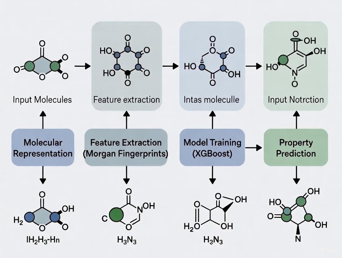
Building a High-Performance Molecular Property Predictor: A Practical Guide to Morgan Fingerprints and XGBoost
This article provides a comprehensive, step-by-step guide for researchers and drug development professionals on constructing a robust molecular property predictor by integrating Morgan fingerprints with the XGBoost algorithm.
Building a High-Performance Molecular Property Predictor: A Practical Guide to Morgan Fingerprints and XGBoost
Abstract
This article provides a comprehensive, step-by-step guide for researchers and drug development professionals on constructing a robust molecular property predictor by integrating Morgan fingerprints with the XGBoost algorithm. It covers the foundational theory behind these techniques, details their practical implementation, and addresses common challenges like data scarcity and hyperparameter tuning. The guide also presents a rigorous framework for model validation and benchmarking against alternative methods, empowering scientists to leverage this powerful, non-deep-learning approach for accelerated drug discovery and materials design.
Understanding the Core Components: Morgan Fingerprints and XGBoost
The Central Role of Molecular Representation
In the field of cheminformatics and drug discovery, molecular representation refers to the process of converting the complex structural information of a chemical compound into a numerical format that machine learning algorithms can process. The fundamental principle, known as the Quantitative Structure-Activity Relationship (QSAR), posits that a molecule's structure determines its properties and biological activity [1]. The choice of representation directly influences a model's ability to capture these structure-property relationships, thereby determining the success of any predictive pipeline.
Molecular representations bridge the gap between chemical structures and machine learning models. For researchers and drug development professionals, selecting an optimal representation is crucial for building accurate predictors for properties such as toxicity, solubility, binding affinity, and odor perception [2] [1]. This document, framed within a broader thesis on building molecular property predictors, details why molecular representation forms the foundational step and provides a detailed protocol for implementing a predictor using the powerful combination of Morgan Fingerprints and the XGBoost algorithm.
Key Molecular Representation Methods
Several molecular representation schemes have been developed, each with distinct strengths and limitations. The table below summarizes the most prominent types used in machine learning applications.
Table 1: Key Molecular Representation Methods for Machine Learning
| Representation Type | Description | Key Advantages | Common Applications |
|---|---|---|---|
| Morgan Fingerprints (ECFP) [2] [1] | Circular topological fingerprints that capture atomic neighborhoods and substructures up to a specified radius. | Captures local structural features invariant to atom numbering; highly effective for similarity search and QSAR. | Drug-target interaction, property prediction, virtual screening. |
| Molecular Descriptors [2] | 1D or 2D numerical values representing physicochemical properties (e.g., molecular weight, logP, polar surface area). | Direct physical meaning; often easily interpretable. | Preliminary screening, models requiring direct physicochemical insight. |
| Functional Group (FG) Fingerprints [2] | Binary vectors indicating the presence or absence of predefined functional groups or substructures. | Simple and interpretable; directly links known chemical features to activity. | Toxicity prediction, metabolic stability. |
| Data-Driven (Deep Learning) Fingerprints [3] [1] | Continuous vector representations learned by deep learning models (e.g., Autoencoders, Transformers) from molecular data. | Can capture complex, non-obvious patterns without manual feature engineering; often high-dimensional. | State-of-the-art property prediction, de novo molecular design. |
| 3D Geometric Representations [4] | Encodes the three-dimensional spatial conformation of a molecule, including atomic coordinates and distances. | Captures stereochemistry and spatial interactions critical for binding affinity. | Protein-ligand docking, binding affinity prediction. |
Among these, Morgan Fingerprints remain one of the most widely used and effective representations, particularly when combined with powerful ensemble tree models like XGBoost [5] [2]. Their success lies in their ability to systematically and comprehensively encode the topological structure of a molecule into a fixed-length bit vector, providing a rich feature set for machine learning algorithms.
Morgan Fingerprints: A Closer Look
The Morgan algorithm, also known as the Extended-Connectivity Fingerprints (ECFP) generation algorithm, operates by iteratively characterizing the environment around each non-hydrogen atom in a molecule [1]. The process can be visualized as a series of circular layers expanding around each atom.
The following diagram illustrates the logical workflow and key parameter choices for generating a Morgan Fingerprint.
The process involves two critical parameters:
- Radius (N): This defines the diameter of the atomic environment considered. A radius of 1 includes the immediate neighbors of an atom, while a radius of 2 includes neighbors of neighbors, capturing larger substructures. Common choices are 2 or 3 [1].
- Fingerprint Length: The size of the final bit vector (e.g., 1024, 2048). A longer vector reduces the chance of hash collisions but increases computational load.
The XGBoost Advantage for Molecular Property Prediction
XGBoost (eXtreme Gradient Boosting) is a highly optimized implementation of the gradient-boosted decision trees algorithm. Its popularity in machine learning competitions and industrial applications stems from its superior performance, speed, and robustness [6] [7].
In the context of molecular property prediction, the high-dimensional, sparse feature vectors produced by Morgan Fingerprints are an excellent match for XGBoost's strengths. The algorithm works by sequentially building decision trees, where each new tree is trained to correct the errors made by the previous ensemble of trees [7].
Key features that make XGBoost particularly effective for this domain include:
- Handling of Sarse Data: It efficiently handles the sparse binary vectors generated by fingerprinting algorithms [6].
- Regularization: Built-in L1 and L2 regularization helps to prevent overfitting, which is a common risk with high-dimensional fingerprint data [5] [7].
- Feature Importance: XGBoost provides built-in tools to calculate feature importance, offering insights into which molecular substructures may be driving the prediction, adding a layer of interpretability [7].
Table 2: Benchmarking Performance of Morgan Fingerprints with XGBoost
| Task / Dataset | Representation - Model | Performance Metric | Result | Citation |
|---|---|---|---|---|
| Odor Prediction | Morgan Fingerprint - XGBoost | AUROC | 0.828 | [2] |
| (Multi-label, 8,681 compounds) | Molecular Descriptors - XGBoost | AUROC | 0.802 | [2] |
| Functional Group - XGBoost | AUROC | 0.753 | [2] | |
| Critical Temperature Prediction | Mol2Vec Embedding - XGBoost | R² | 0.93 | [8] |
| (CRC Handbook Dataset) | VICGAE Embedding - XGBoost | R² | Comparable | [8] |
| Embedded Morgan (eMFP) | eMFP (q=16/32/64) - Multiple Models | Regression Performance | Outperformed standard MFP | [5] |
| (RedDB, NFA, QM9 Databases) |
As evidenced in the table above, the combination of Morgan Fingerprints and XGBoost consistently delivers high performance across diverse molecular property prediction tasks, from complex sensory attributes like odor to fundamental physical properties.
Experimental Protocol: Building a MorganFP-XGBoost Predictor
This section provides a detailed, step-by-step protocol for building a molecular property predictor using Morgan Fingerprints and XGBoost.
The Scientist's Toolkit: Essential Research Reagents & Software
Table 3: Essential Tools and Libraries for Implementation
| Item Name | Function / Purpose | Example / Notes |
|---|---|---|
| RDKit | Open-source cheminformatics toolkit. | Used for reading molecules, generating Morgan fingerprints, and calculating molecular descriptors. Essential for the protocol [2] [8] [1]. |
| XGBoost Library | Python/R/Julia library implementing the XGBoost algorithm. | Provides the XGBRegressor and XGBClassifier for model building. Optimized for performance [6] [7]. |
| Scikit-learn | Machine learning library in Python. | Used for data splitting, preprocessing, cross-validation, and performance metric calculation. |
| Python/Pandas/NumPy | Programming language and data manipulation libraries. | The core environment for scripting the data pipeline and analysis. |
| Molecular Dataset | Curated set of molecules with associated property data. | Public sources: DrugBank, ChEMBL, PubChem, CRC Handbook [8]. Requires SMILES strings and target property values. |
Step-by-Step Workflow
The following diagram outlines the complete machine learning pipeline, from raw data to a trained and validated predictive model.
Protocol Steps:
Data Curation and Preprocessing
- Input: A dataset containing canonical SMILES (Simplified Molecular Input Line Entry System) strings and the corresponding target property values (e.g., boiling point, toxicity label) [8].
- Action: Standardize the molecules using RDKit. This includes sanitizing the molecular graph, removing salts, and generating canonical SMILES. Handle missing values and outliers in the target property.
Generate Morgan Fingerprints
- Action: Use the RDKit's
GetMorganFingerprintAsBitVectfunction to convert each SMILES string into a fixed-length binary bit vector. - Critical Parameters:
radius: Typically set to 2 or 3. This controls the level of structural detail captured.nBits: The length of the fingerprint vector. A value of 1024 or 2048 is commonly used to balance specificity and computational cost [3].
- Action: Use the RDKit's
Split Data
- Action: Split the dataset into training, validation, and test sets. A scaffold split, which separates molecules based on their core Bemis-Murcko scaffolds, is recommended to rigorously test the model's ability to generalize to novel chemotypes [4]. A typical ratio is 80/10/10.
Hyperparameter Tuning
- Action: Use the training set to train XGBoost models and the validation set to guide hyperparameter optimization. Employ frameworks like Optuna or GridSearchCV for an efficient search [8].
- Key XGBoost Hyperparameters:
max_depth: Maximum depth of a tree (e.g., 3-10). Controls model complexity.learning_rate(eta): Shrinks the contribution of each tree (e.g., 0.01-0.3).n_estimators: Number of boosting rounds. Useearly_stopping_roundsto prevent overfitting.subsample: Fraction of samples used for training each tree.colsample_bytree: Fraction of features (fingerprint bits) used per tree.
Train Final Model
- Action: Using the best-found hyperparameters, train the final XGBoost model on the combined training and validation data.
Evaluate Model
- Action: Make predictions on the held-out test set, which was not used during training or tuning. Report standard performance metrics:
- Regression (e.g., for boiling point): R², Mean Absolute Error (MAE), Root Mean Squared Error (RMSE).
- Classification (e.g., for toxicity): AUC-ROC, Accuracy, Precision, Recall, F1-Score.
- Action: Make predictions on the held-out test set, which was not used during training or tuning. Report standard performance metrics:
Analyze Feature Importance
- Action: Use XGBoost's built-in
feature_importance_attribute (e.g.,gaintype) to identify the fingerprint bits (and by extension, the molecular substructures) that were most influential in the model's predictions. This can provide valuable chemical insights.
- Action: Use XGBoost's built-in
Advanced Techniques and Future Directions
As the field advances, several techniques are being developed to enhance the basic Morgan-XGBoost pipeline:
- Embedded Morgan Fingerprints (eMFP): This method applies dimensionality reduction to standard Morgan fingerprints, creating a lower-dimensional, continuous representation. eMFP has been shown to mitigate overfitting and can outperform standard MFP, especially with regression models [5].
- Deep Learning Representations: Methods like FP-BERT treat fingerprint substructures as words in a sentence and use transformer-based models to learn contextualized molecular representations in a self-supervised manner before fine-tuning on specific tasks [1]. Other advanced models like SCAGE incorporate 3D conformational information and functional group knowledge through multi-task pre-training, leading to improved generalization and interpretability on challenging structure-activity cliffs [4].
In conclusion, molecular representation is the indispensable first step in any computational prediction of molecular properties. The robust and interpretable combination of Morgan Fingerprints for feature extraction and XGBoost for model building provides a powerful, reliable, and accessible pipeline for researchers. This protocol offers a solid foundation, while emerging techniques in dimensionality reduction and deep learning promise to further push the boundaries of predictive accuracy and chemical insight.
Molecular fingerprints are essential cheminformatics tools that encode the structural features of a molecule into a fixed-length vector, enabling quantitative similarity comparisons and machine learning applications in drug discovery [9] [10]. Among the various types of fingerprints, the Morgan fingerprint, also known as the Extended Connectivity Fingerprint (ECFP), stands out for its effectiveness in capturing circular atom neighborhoods within molecular structures [11]. These fingerprints operate on the fundamental principle that molecules with similar substructures often exhibit similar biological activities or physicochemical properties, making them invaluable for quantitative structure-activity relationship (QSAR) modeling and virtual screening [9].
The Morgan algorithm, originally developed to tackle graph isomorphism problems, provides the theoretical foundation for these fingerprints [12] [11]. Unlike predefined structural keys (e.g., MACCS keys) that test for the presence of specific expert-defined substructures, Morgan fingerprints are molecule-directed and generated systematically from the molecular graph itself without requiring a predefined fragment library [11] [10]. This allows them to capture a vast and relevant set of chemical features directly from the data, which is particularly advantageous for predicting complex molecular properties when combined with powerful machine learning algorithms like XGBoost [2] [12].
Theoretical Foundation and Generation Algorithm
Core Conceptual Framework
The Morgan fingerprint generation process employs a circular topology approach that systematically captures information about the neighborhood around each non-hydrogen atom in a molecule [11]. The algorithm is rooted in the concept of circular atom environments, which represent the substructures within a progressively increasing radius around each atom. This approach allows the fingerprint to encode molecular features at multiple levels of granularity, from individual atomic properties to larger functional groupings [13] [11].
A key advantage of this circular approach is its alignment invariance - unlike 3D structural representations that require molecular alignment for comparison, Morgan fingerprints derive directly from the 2D molecular graph, enabling rapid similarity calculations without spatial orientation concerns [13]. Additionally, the representation is deterministic, meaning the same molecule will always generate the same fingerprint, ensuring reproducibility in chemical informatics workflows [11].
Step-by-Step Generation Process
The Morgan fingerprint generation follows a systematic iterative process:
Initial Atom Identifier Assignment: The algorithm begins by assigning an initial integer identifier to each non-hydrogen atom in the molecule. This identifier encapsulates key local atom properties, typically including: atomic number, number of heavy (non-hydrogen) neighbors, number of attached hydrogens (both implicit and explicit), formal charge, and whether the atom is part of a ring [11]. These properties are hashed into a single integer value using a hash function.
Iterative Identifier Updating: The algorithm then performs a series of iterations to capture progressively larger circular neighborhoods around each atom. At each iteration, the current identifier for an atom is updated by combining it with the identifiers of its directly connected neighbors. This combined information is then hashed to produce a new integer identifier representing a larger substructure [11] [14]. The number of iterations determines the maximum diameter of the captured circular neighborhoods.
Feature Collection and Duplicate Removal: All unique integer identifiers generated throughout the iterations (including the initial ones) are collected into a set. Each identifier represents a distinct circular substructure present in the molecule. By default, duplicate occurrences of the same substructure are recorded only once, though the algorithm can be configured to keep count frequencies (resulting in ECFC - Extended Connectivity Fingerprint Count) [11].
Fingerprint Folding (Optional): The final set of integer identifiers can be used directly as a variable-length fingerprint. However, for easier storage and comparison, it is commonly "folded" into a fixed-length bit vector (e.g., 1024 or 2048 bits) using a modulo operation [13] [11]. This step makes the fingerprint more compact but may introduce bit collisions, where different substructures map to the same bit position.
Table 1: Key Parameters in Morgan Fingerprint Generation
| Parameter | Description | Typical Values | Impact on Fingerprint |
|---|---|---|---|
| Diameter | Maximum diameter of circular neighborhoods | 2, 4, 6 | Larger values capture larger substructures, increasing specificity |
| Length | Size of folded bit vector | 512, 1024, 2048 | Longer vectors reduce bit collisions and information loss |
| Atom Features | Properties encoded in initial identifier | Atomic number, connectivity, charge, etc. | Determines the chemical features represented |
| Counts | Whether to record feature frequencies | Yes/No | Count fingerprints may capture additional information |
Figure 1: Morgan Fingerprint Generation Workflow - This diagram illustrates the systematic process of generating Morgan fingerprints from 2D molecular structures through iterative neighborhood expansion.
Integration with Machine Learning (XGBoost) for Property Prediction
Synergy Between Morgan Fingerprints and XGBoost
The combination of Morgan fingerprints and XGBoost (eXtreme Gradient Boosting) has emerged as a powerful framework for molecular property prediction in modern cheminformatics [2] [12]. This synergy leverages the complementary strengths of both technologies: Morgan fingerprints effectively capture relevant chemical structures in a numerically encoded format, while XGBoost efficiently learns complex, non-linear patterns from these high-dimensional, sparse encodings [2]. The gradient-boosting approach of XGBoast is particularly well-suited to handle the sparse, binary nature of fingerprint vectors, with built-in regularization that helps prevent overfitting even when using high-dimensional feature spaces [2] [12].
Recent benchmark studies have demonstrated the exceptional performance of this combination across diverse prediction tasks. In odor perception prediction, a Morgan-fingerprint-based XGBoost model achieved an area under the receiver operating characteristic curve (AUROC) of 0.828 and an area under the precision-recall curve (AUPRC) of 0.237, outperforming both descriptor-based models and other machine learning algorithms [2]. Similarly, in ADME-Tox (absorption, distribution, metabolism, excretion, and toxicity) prediction, this combination delivered competitive performance across multiple endpoints including Ames mutagenicity, P-glycoprotein inhibition, and hERG inhibition [12].
Protocol: Building a Molecular Property Predictor
Protocol 1: Molecular Property Prediction Using Morgan Fingerprints and XGBoost
Purpose: To construct a robust machine learning model for predicting molecular properties using Morgan fingerprints as features and XGBoost as the learning algorithm.
Materials and Software Requirements:
- Chemical Dataset: Curated set of molecules with associated property/activity data (e.g., from ChEMBL, PubChem)
- Cheminformatics Library: RDKit (for fingerprint generation and molecular processing)
- Machine Learning Library: XGBoost package
- Computational Environment: Python with standard data science libraries (pandas, numpy, scikit-learn)
Procedure:
Data Curation and Preprocessing:
- Obtain molecular structures in SMILES (Simplified Molecular Input Line Entry System) format with associated target property values.
- Apply standard chemical curation: remove duplicates, strip salts, and filter by element composition (typically C, H, N, O, S, P, F, Cl, Br, I) [12].
- For unbalanced datasets, consider applying techniques such as oversampling or undersampling to balance class distributions [12].
Feature Generation (Fingerprinting):
- Generate Morgan fingerprints for each molecule using RDKit's
GetMorganFingerprintAsBitVectfunction. - Use a diameter of 4 (equivalent to radius 2) and a fingerprint length of 1024 bits as starting parameters [11].
- Consider testing alternative parameters (diameter of 2 or 6, lengths of 512 or 2048) to optimize for specific applications.
- Convert the fingerprints into a feature matrix where each row represents a molecule and each column represents a bit position.
- Generate Morgan fingerprints for each molecule using RDKit's
Model Training and Validation:
- Split the dataset into training (80%) and test (20%) sets, maintaining class distribution through stratified sampling [2].
- Implement 5-fold cross-validation on the training set for robust hyperparameter tuning and model selection.
- Configure XGBoost with appropriate parameters for the task (binary classification, multiclass, or regression).
- Train the XGBoost model on the fingerprint feature matrix, using the target property as the response variable.
Model Evaluation and Interpretation:
- Evaluate model performance on the held-out test set using task-appropriate metrics: AUROC and AUPRC for classification; RMSE and R² for regression.
- Analyze feature importance scores provided by XGBoost to identify which structural features most strongly influence predictions.
- Validate model applicability domain by assessing performance consistency across diverse chemical scaffolds.
Troubleshooting Tips:
- If model performance is poor, consider increasing fingerprint diameter to capture larger substructures or adjusting XGBoost hyperparameters (learning rate, maximum depth, number of estimators).
- For datasets with strong class imbalance, adjust XGBoost's
scale_pos_weightparameter or employ specialized sampling techniques. - If overfitting occurs, increase regularization parameters (lambda, alpha) or reduce model complexity.
Performance Benchmarking and Applications
Quantitative Performance Across Domains
Morgan fingerprints have demonstrated competitive performance across diverse chemical informatics applications. The following table summarizes benchmark results from recent studies:
Table 2: Performance Benchmarks of Morgan Fingerprints in Various Applications
| Application Domain | Dataset | Performance Metrics | Comparative Performance |
|---|---|---|---|
| Odor Perception | 8,681 compounds from 10 expert sources [2] | AUROC: 0.828, AUPRC: 0.237 [2] | Superior to functional group and molecular descriptor approaches [2] |
| ADME-Tox Prediction | 6 binary classification targets (1,000-6,500 molecules each) [12] | Competitive across multiple endpoints [12] | Comparable or superior to other fingerprint types (MACCS, Atompairs) [12] |
| Drug Target Prediction | ChEMBL20 database [13] | Higher precision-recall than 3D fingerprints (E3FP) in some cases [13] | Complementary to 3D structural information [13] |
| Virtual Screening | Multiple benchmark studies [11] | Among best performing for similarity searching [11] | Typically outperforms path-based fingerprints for similarity searching [11] |
Application Notes in Drug Discovery
Application Note 1: Scaffold Hopping and Bioactivity Prediction
Morgan fingerprints excel in identifying structurally diverse compounds with similar bioactivity - a process known as scaffold hopping. Their circular substructure representation captures pharmacophoric features essential for binding without being constrained by molecular backbone identity [11]. When implementing scaffold hopping:
- Use a shorter fingerprint diameter (2-4) to focus on key pharmacophoric elements rather than complete scaffold structures
- Combine similarity searching with machine learning by training XGBoost models on known actives and inactives
- Apply similarity thresholds (Tanimoto coefficient > 0.4-0.6) to identify promising candidates from virtual screens [11]
Application Note 2: ADME-Tox Optimization in Lead Series
In lead optimization, Morgan fingerprints facilitate the prediction of absorption, distribution, metabolism, excretion, and toxicity (ADME-Tox) properties [12] [11]. Implementation guidelines include:
- Train separate XGBoost models for specific ADME-Tox endpoints (e.g., hERG inhibition, CYP450 interactions)
- Use larger fingerprint diameters (4-6) to capture complex structural features influencing metabolic stability
- Interpret feature importance to guide structural modifications that improve safety profiles while maintaining potency
- Integrate multiple property predictions into multi-parameter optimization workflows [12]
Figure 2: Integrated Workflow for Molecular Property Prediction - This diagram outlines the complete pipeline from molecular structure input to property prediction, highlighting key application domains where Morgan fingerprints combined with XGBoost deliver strong performance.
Table 3: Essential Tools and Resources for Implementing Morgan Fingerprint-Based Predictions
| Resource Category | Specific Tool/Resource | Key Function | Implementation Notes |
|---|---|---|---|
| Cheminformatics Libraries | RDKit [12] [14] | Open-source toolkit for fingerprint generation and molecular processing | Provides GetMorganFingerprintAsBitVect function with configurable parameters |
| Machine Learning Frameworks | XGBoost [2] [12] | Gradient boosting library for building predictive models | Handles sparse fingerprint data efficiently with built-in regularization |
| Chemical Databases | ChEMBL [13] [3], PubChem [2] | Sources of curated molecular structures with bioactivity data | Provide standardized datasets for model training and validation |
| Specialized Fingerprints | E3FP (3D fingerprints) [13] | 3D structural fingerprints for specific applications | Complementary to Morgan fingerprints for certain target classes |
| Similarity Metrics | Tanimoto coefficient [9] | Measure fingerprint similarity for virtual screening | Default similarity metric for binary fingerprint comparisons |
| Model Validation | Scikit-learn [2] | Machine learning utilities for model evaluation | Provides cross-validation and performance metric implementations |
Advanced Considerations and Future Directions
Limitations and Complementary Approaches
Despite their widespread success, Morgan fingerprints have limitations that researchers should consider in advanced applications. Their 2D topological nature means they cannot directly capture molecular shape, conformation, or stereochemical features that may critically influence biological activity [13]. For targets where 3D structure is crucial, consider complementary approaches such as:
- E3FP (Extended Three-Dimensional FingerPrint): A 3D extension of Morgan fingerprints that captures stereochemistry and spatial relationships [13]
- Structural Interaction Fingerprints: Encode protein-ligand interaction patterns from 3D complex structures [9]
- Hybrid representations: Combine Morgan fingerprints with molecular descriptors or 3D information for enhanced predictive capability [15]
Additionally, the dependence on hashing functions means that different implementations may produce varying results, and the folding process can introduce bit collisions that reduce discriminative power [11]. For large-scale applications, consider using unfolded fingerprints or increased vector lengths (2048+ bits) to minimize collisions.
Emerging Trends and Methodological Advances
The field of molecular representation continues to evolve with several promising directions:
- Hybrid fingerprint-graph models: Recent approaches like Fingerprint-Enhanced Hierarchical Molecular Graph Neural Networks (FH-GNN) integrate Morgan fingerprints with graph neural networks to capture both local functional groups and global molecular topology [15]
- Multi-task learning: Training single models on multiple related endpoints using Morgan fingerprints as common input features [3]
- Universal fingerprints: Development of representations like MAP4 (MinHashed Atom-Pair fingerprint) that aim to perform well across diverse molecule types, from small drugs to biomacromolecules [16]
- Interpretability advances: Improved methods for mapping important fingerprint bits back to chemically meaningful substructures, enhancing model trustworthiness in decision-critical applications [9] [15]
As these advances mature, Morgan fingerprints remain a fundamental tool in the cheminformatics toolbox, providing a robust, interpretable, and computationally efficient foundation for molecular machine learning that continues to deliver state-of-the-art performance across diverse applications in drug discovery and chemical informatics.
In the field of computational chemistry and drug discovery, accurately predicting molecular properties from chemical structure is a fundamental challenge. The combination of Morgan fingerprints for molecular representation and the XGBoost algorithm for model building has emerged as a particularly powerful and popular approach. This synergy provides researchers with a robust framework for building predictive models that can accelerate virtual screening and compound optimization [2].
Morgan fingerprints, also known as circular fingerprints, capture molecular structure by encoding the presence of specific substructures and atomic environments within a molecule. When paired with XGBoost, an advanced gradient boosting implementation known for its computational efficiency and predictive performance, they form a potent combination for tackling quantitative structure-activity relationship (QSAR) and quantitative structure-property relationship (QSPR) tasks [2] [5].
This protocol outlines the application of these tools for building molecular property predictors, providing a structured guide from data preparation to model deployment, supported by recent benchmarking studies demonstrating their effectiveness.
Key Evidence: Performance Benchmarks
Recent comparative studies have quantitatively demonstrated the superiority of XGBoost models utilizing Morgan fingerprints across various molecular prediction tasks.
Table 1: Performance comparison of feature representation and algorithm combinations for odor prediction [2]
| Feature Set | Algorithm | AUROC | AUPRC | Accuracy (%) | Precision (%) | Recall (%) |
|---|---|---|---|---|---|---|
| Morgan Fingerprints (ST) | XGBoost | 0.828 | 0.237 | 97.8 | 41.9 | 16.3 |
| Morgan Fingerprints (ST) | LightGBM | 0.810 | 0.228 | - | - | - |
| Morgan Fingerprints (ST) | Random Forest | 0.784 | 0.216 | - | - | - |
| Molecular Descriptors (MD) | XGBoost | 0.802 | 0.200 | - | - | - |
| Functional Group (FG) | XGBoost | 0.753 | 0.088 | - | - | - |
This comprehensive study analyzed 8,681 compounds with 200 odor descriptors, revealing that the Morgan-fingerprint-based XGBoost model achieved the highest discrimination performance, consistently outperforming both descriptor-based models and other algorithmic approaches [2].
Table 2: Performance of XGBoost across different domains
| Application Domain | Dataset/Setting | Key Performance Metrics | Citation |
|---|---|---|---|
| Thyroid Nodule Malignancy Prediction | Clinical & ultrasound features (n=2,014) | AUC: 0.928, Accuracy: 85.1%, Sensitivity: 93.3% | [17] |
| Physical Fitness Classification | 20,452 student records | Accuracy, Recall, F1: 3.5-7.9% improvement over baselines | [18] |
| STAT3 Inhibitor Prediction | FPG model with fingerprint integration | Average AUC: 0.897 on test set | [19] |
Technical Synergy: Why XGBoost and Morgan Fingerprints Work Well Together
Complementary Strengths
The effectiveness of this combination stems from how well the strengths of Morgan fingerprints align with the capabilities of the XGBoost algorithm:
High-Dimensional Sparse Data Handling: Morgan fingerprints typically generate high-dimensional binary vectors (often 1,024 to 2,048 dimensions) where most bits are zero. XGBoost efficiently handles such sparse data structures through its built-in sparsity-aware split finding algorithm [2] [20].
Non-Linear Relationship Capture: Molecular properties often depend on complex, non-linear interactions between structural features. XGBoost's sequential tree building with gradient optimization excels at detecting these patterns, outperforming linear models and single decision trees [2].
Robustness and Regularization: The molecular space is diverse, with potential for overfitting. XGBoost incorporates L1 and L2 regularization directly into its objective function, preventing overfitting on the high-dimensional fingerprint data [2] [18].
Computational Efficiency: For medium-sized molecular datasets (typically thousands to tens of thousands of compounds), XGBoost provides faster training times compared to deep learning approaches while maintaining competitive performance [20].
Recent Methodological Advances
Recent research has further optimized this partnership:
Embedded Morgan Fingerprints (eMFP): A novel dimensionality reduction technique that compresses standard Morgan fingerprints while preserving key structural information. This approach has demonstrated improved performance in regression models across multiple databases including RedDB, NFA, and QM9 [5].
Hybrid Architectures: New frameworks like MaxQsaring automate the selection of optimal feature combinations, including molecular descriptors, fingerprints, and deep-learning pretrained representations, with XGBoost frequently emerging as the top performer for prediction tasks [21].
Integration with Graph Neural Networks: Fingerprint-enhanced graph neural networks (e.g., FPG models) concatenate learned graph representations with traditional fingerprint vectors, with XGBoost often serving as the final prediction layer in such architectures [19].
Application Notes & Protocols: Building a Molecular Property Predictor
The following diagram illustrates the complete workflow for building a molecular property predictor using Morgan fingerprints and XGBoost:
Protocol 1: Data Preparation and Morgan Fingerprint Generation
Materials and Software Requirements
Table 3: Essential software tools and libraries
| Tool/Library | Purpose | Installation Command |
|---|---|---|
| RDKit | Chemical informatics and fingerprint generation | conda install -c conda-forge rdkit |
| XGBoost | Gradient boosting model implementation | pip install xgboost |
| Pandas & NumPy | Data manipulation and numerical operations | pip install pandas numpy |
| Scikit-learn | Data splitting, preprocessing, and evaluation metrics | pip install scikit-learn |
Step-by-Step Procedure
Data Collection and Standardization
- Obtain molecular structures in SMILES (Simplified Molecular Input Line Entry System) format from databases such as PubChem, ChEMBL, or in-house collections.
- Standardize SMILES representation using RDKit's
Chem.MolToSmiles(Chem.MolFromSmiles(smile))to ensure consistency. - Curate associated molecular property data (e.g., activity labels, solubility values, toxicity measurements).
Morgan Fingerprint Generation
- Use RDKit to compute Morgan fingerprints with a radius of 2 (equivalent to ECFP4) and 1024-bit length:
- For larger datasets (>10,000 compounds), consider using embedded Morgan fingerprints (eMFP) with compression sizes of q=16, 32, or 64 to reduce dimensionality while preserving structural information [5].
Data Splitting
- Implement scaffold splitting using RDKit's
ScaffoldSplitterto ensure training and test sets contain distinct molecular scaffolds, providing a more realistic assessment of generalization ability. - Standard alternative: Use random 80/20 split for training/test sets with stratification for classification tasks to maintain class distribution.
- Implement scaffold splitting using RDKit's
Protocol 2: XGBoost Model Development and Optimization
Materials and Software Requirements
- Python 3.7+ environment with xgboost package (v1.7+)
- Hyperparameter optimization library (Optuna, Scikit-optimize, or GridSearchCV)
Step-by-Step Procedure
Base Model Configuration
- Initialize XGBoost with parameters suitable for molecular data:
Hyperparameter Optimization
- Employ differential evolution (DE) for global parameter optimization, which has shown superior performance for XGBoost tuning on high-dimensional data [18].
- Key hyperparameters to optimize:
max_depth(3-10): Tree complexity balancelearning_rate(0.01-0.3): Step size shrinkagesubsample(0.6-1.0): Data sampling ratioreg_alphaandreg_lambda(0-1): Regularization strengthsn_estimators(50-500): Number of boosting rounds
Model Training with Cross-Validation
- Implement stratified k-fold cross-validation (k=5 or 10) to robustly estimate performance.
- Use early stopping to prevent overfitting:
eval_set=[(X_test, y_test)],early_stopping_rounds=50.
Protocol 3: Model Evaluation and Interpretation
Materials and Software Requirements
- Model evaluation metrics (AUROC, AUPRC, accuracy, precision, recall)
- SHAP library for model interpretation
- Matplotlib/Seaborn for visualization
Step-by-Step Procedure
Performance Assessment
- Calculate standard metrics: Area Under Receiver Operating Characteristic curve (AUROC), Area Under Precision-Recall Curve (AUPRC), accuracy, precision, and recall.
- Generate calibration curves to assess prediction reliability.
- Perform decision curve analysis to evaluate clinical utility where applicable [17].
Model Interpretation
- Apply SHAP (SHapley Additive exPlanations) to identify which molecular substructures (fingerprint bits) most strongly influence predictions.
- Analyze feature importance scores generated by XGBoost's built-in method.
- Visualize key molecular fragments associated with activity using RDKit's chemical visualization capabilities.
Model Deployment
- Serialize the trained model using
pickleorjoblibfor production use. - For web applications, deploy using frameworks like Flask or FastAPI, or create R Shiny applications for non-programming users [17].
- Serialize the trained model using
Table 4: Key resources for building molecular predictors with Morgan fingerprints and XGBoost
| Resource | Type | Purpose/Function | Availability |
|---|---|---|---|
| RDKit | Software Library | Chemical informatics and fingerprint generation | Open-source (BSD license) |
| PyRfume | Data Resource | Curated olfactory dataset with 8,681 compounds | GitHub: pyrfume/pyrfume-data [2] |
| PubChem PUG-REST | API | SMILES retrieval and molecular data access | https://pubchem.ncbi.nlm.nih.gov/ [2] |
| XGBoost | Software Library | Gradient boosting model implementation | Open-source (Apache License 2.0) |
| Therapeutics Data Commons (TDC) | Benchmark Platform | Standardized datasets for fair model comparison | https://tdc.ai/ [21] |
| SHAP Library | Interpretation Tool | Model explanation and feature importance | Open-source (MIT License) |
Technical Considerations and Advanced Applications
Addressing Limitations
While powerful, the Morgan fingerprint + XGBoost approach has limitations:
Activity Cliffs: Subtle structural changes causing dramatic property changes may be better captured by 3D molecular representations or graph neural networks incorporating spatial information [4].
Novel Scaffolds: Performance may decrease for entirely novel molecular scaffolds not represented in training data. Consider transfer learning or multitask learning approaches.
High-Dimensionality Challenges: For extremely high-dimensional fingerprints, consider embedded Morgan fingerprints (eMFP) which offer compressed representations while maintaining performance [5].
Emerging Hybrid Approaches
Recent research demonstrates promising directions combining the strengths of this approach with advanced deep learning:
Fingerprint-Enhanced Graph Neural Networks: Architectures that simultaneously process graph representations and traditional fingerprints, with XGBoost sometimes used as the final predictor [15] [19].
Multimodal Representations: Integrating Morgan fingerprints with additional molecular representations (descriptors, pretrained deep learning representations) in frameworks like MaxQsaring, which automatically select optimal feature combinations [21].
Self-Conformation-Aware Models: Approaches like SCAGE that incorporate 3D conformational information while maintaining interpretability through attention mechanisms [4].
The combination of Morgan fingerprints and XGBoost represents a robust, interpretable, and high-performing approach for molecular property prediction that continues to deliver state-of-the-art results across diverse applications. While newer deep learning methods offer promise for specific challenges, the simplicity, computational efficiency, and proven performance of this established methodology make it an essential tool in computational chemistry and drug discovery. The protocols and applications detailed in this document provide researchers with a comprehensive framework for implementing this powerful approach in their molecular prediction workflows.
Accurate molecular property prediction is a cornerstone of modern drug discovery, enabling researchers to identify promising compounds while reducing the costs and risks associated with experimental trials [22]. In this context, the selection of an optimal molecular representation and machine learning algorithm is paramount. This application note synthesizes recent evidence demonstrating that the combination of Morgan Fingerprints (MFP) as molecular descriptors with the XGBoost algorithm constitutes a particularly powerful and efficient approach for building predictive models in cheminformatics. While novel deep learning methods have garnered significant attention, systematic evaluations reveal that traditional machine learning methods, when paired with high-quality engineered features like Morgan Fingerprints, often deliver superior or highly competitive performance with greater computational efficiency [23] [22]. We present quantitative benchmarks, detailed protocols, and practical resources to empower researchers to implement this robust methodology in their molecular property prediction workflows.
Performance Evidence and Comparative Analysis
Recent comprehensive studies provide strong empirical support for the Morgan Fingerprint and XGBoost combination across diverse molecular property prediction tasks.
Systematic Benchmarking on Molecular Datasets
A large-scale systematic study evaluated numerous representation learning models and fixed representations across MoleculeNet datasets and opioids-related datasets. After training over 62,000 models, the study concluded that representation learning models exhibit limited performance in most molecular property prediction datasets and highlighted that dataset size is crucial for model success [23]. This finding underscores the advantage of using robust traditional methods like XGBoost with Morgan Fingerprints, especially in lower-data regimes common in early-stage drug discovery.
Table 1: Performance of Fingerprint-Based Methods in Recent Studies
| Study | Dataset(s) | Key Finding | Implication for MFP+XGBoost |
|---|---|---|---|
| He et al. (2025) [24] | ChEMBL 34 (FDA-approved drugs) | MolTarPred using Morgan fingerprints with Tanimoto scores was the most effective target prediction method. | Validates Morgan fingerprints as a superior choice for ligand-centric prediction tasks. |
| Embedded MFP (2025) [5] | RedDB, NFA, QM9 | Embedded Morgan Fingerprints (eMFP) outperformed standard MFP in multiple regression models, including Gradient Booster Regressor. | Suggests potential for dimensionality-reduced MFP to further enhance tree-based models. |
| Deng et al. (2023) [23] | MoleculeNet, Opioids datasets | Representation learning models showed limited performance; fixed representations like fingerprints remain highly competitive. | Affirms that advanced feature engineering (e.g., MFP) with classical ML is a robust strategy. |
| FH-GNN (2025) [22] | 8 MoleculeNet datasets | Integrating fingerprints with graph models (FH-GNN) boosted performance, showing fingerprints provide complementary information. | Highlights the strong predictive priors encoded in fingerprints, which XGBoost can effectively leverage. |
Enhanced Morgan Fingerprints for Improved Performance
A novel approach termed Embedded Morgan Fingerprints (eMFP) has been developed to address challenges of high-dimensionality in standard MFP. eMFP applies dimensionality reduction to the Morgan Fingerprint while preserving key structural information, resulting in an improved data representation that mitigates overfitting and enhances model performance [5]. This method demonstrated superior performance over standard MFP across several regression models, including Random Forest and Gradient Booster Regressor, on three different databases (RedDB, NFA, and QM9), with optimal compression sizes of 16, 32, and 64 [5]. The success of eMFP with gradient-boosted models directly reinforces the potential of the MFP-XGBoost combination.
Critical Role in State-of-the-Art Prediction Methods
In a precise 2025 comparison of seven molecular target prediction methods, MolTarPred emerged as the most effective method. A key finding was that its performance was optimized when using Morgan fingerprints with Tanimoto scores, which outperformed the alternative MACCS fingerprints with Dice scores [24]. This result provides direct, recent evidence for the superiority of Morgan fingerprints in a critical, practical application—target prediction for drug repurposing.
Experimental Protocols
Protocol 1: Building a Baseline MFP-XGBoost Predictor
This protocol details the steps to construct a molecular property predictor using standard Morgan Fingerprints and XGBoost.
Workflow Diagram: Baseline MFP-XGBoost Predictor
Step-by-Step Procedure:
- Input Data Preparation: Begin with a dataset of molecules represented as canonical SMILES strings and their associated property values (e.g., IC50, solubility) [24].
- Fingerprint Generation: Using a cheminformatics toolkit like RDKit, generate the Morgan Fingerprint (also known as ECFP, Extended-Connectivity Fingerprint) for each molecule. Standard parameters are a radius of 2 (equivalent to ECFP4) and a bit vector length of 2048 [23] [24].
- Code Snippet (RDKit):
- Data Splitting: Split the dataset into training and testing sets (e.g., 80/20 split). For robust performance estimation, implement a k-fold cross-validation strategy (e.g., 5-fold).
- Model Instantiation: Instantiate an XGBoost regressor or classifier, depending on the nature of the prediction task (continuous or categorical).
- Code Snippet (XGBoost):
- Hyperparameter Tuning: Perform a grid or random search to optimize key hyperparameters. Critical parameters for XGBoost include:
n_estimators: Number of boosting rounds (e.g., 100-1000).max_depth: Maximum tree depth (e.g., 3-10).learning_rate: Shrinks the feature weights to prevent overfitting (e.g., 0.01-0.3).subsample: Fraction of samples used for fitting trees (e.g., 0.8-1.0).
- Model Training: Train the tuned XGBoost model on the entire training set.
- Prediction and Evaluation: Use the trained model to make predictions on the held-out test set. Evaluate performance using relevant metrics: Root Mean Square Error (RMSE) or Mean Absolute Error (MAE) for regression, and ROC-AUC for classification [23].
Protocol 2: Advanced Protocol with Embedded MFP
This protocol leverages the enhanced version of Morgan Fingerprints for potentially superior performance, especially with large datasets.
Workflow Diagram: Advanced Protocol with eMFP
Step-by-Step Procedure:
- Generate Standard MFP: As in Protocol 1, generate the high-dimensional standard Morgan Fingerprint.
- Dimensionality Reduction: Apply a dimensionality reduction technique to create the Embedded Morgan Fingerprint (eMFP). This can be achieved via autoencoders or other compression algorithms. The goal is to reduce the bit vector (e.g., from 2048 bits) to a smaller, dense vector representation (e.g., 16, 32, or 64 dimensions), which preserves the essential structural information while mitigating the curse of dimensionality [5].
- Model Training with eMFP: Use the resulting eMFP vectors as features for the XGBoost model. Follow the same steps for data splitting, hyperparameter tuning, and training as outlined in Protocol 1.
- Performance Comparison: Benchmark the performance of the eMFP-XGBoost model against the baseline MFP-XGBoost model to validate the improvement in predictive accuracy and training efficiency.
The Scientist's Toolkit: Essential Research Reagents
Table 2: Key Software and Data Resources for MFP-XGBoost Modeling
| Resource Name | Type | Function in Workflow | Reference/Source |
|---|---|---|---|
| RDKit | Cheminformatics Library | Generates canonical SMILES from structural files and computes Morgan Fingerprints. | [23] [22] |
| XGBoost Library | Machine Learning Library | Provides the scalable and efficient implementation of the Gradient Boosting algorithm. | [22] |
| ChEMBL Database | Bioactivity Database | Provides a large, curated source of bioactive molecules, targets, and properties for model training and validation. | [23] [24] |
| MoleculeNet | Benchmark Suite | Offers a standardized collection of molecular property prediction datasets for fair model comparison. | [23] [22] |
| Morgan/ECFP Fingerprint | Molecular Representation | Encodes molecular structure into a fixed-length bit vector that captures circular substructures. | [23] [5] [24] |
The accumulated evidence from recent, rigorous comparisons makes a compelling case for the combination of Morgan Fingerprints and XGBoost as a robust and often superior framework for molecular property prediction. This approach consistently delivers high performance, challenging the assumption that more complex deep learning models are invariably better [23]. The robustness of Morgan Fingerprints is further validated by their role in enhancing state-of-the-art graph neural networks [22] and their critical contribution to the top-performing target prediction method, MolTarPred [24].
For researchers and drug development professionals, this combination offers a pragmatic and powerful path forward. It balances predictive accuracy with computational efficiency and model interpretability. The protocols provided herein offer a clear roadmap for implementation, from a baseline model to an advanced variant using embedded MFP. By leveraging this winning combination, scientists can accelerate their cheminformatics workflows and make more reliable predictions to guide the discovery of new therapeutic candidates.
Molecular property prediction is a critical task in drug discovery and chemical sciences, enabling the rapid screening of compounds and accelerating the identification of promising candidates [25] [8]. The core challenge lies in transforming molecular structures into numerical representations that machine learning algorithms can process. The choice of molecular representation significantly influences the predictive performance, interpretability, and computational efficiency of the resulting models [26] [2]. This application note provides a comparative overview of three dominant representation paradigms: expert-crafted descriptors and fingerprints, learned graph-based representations, and features extracted from large language models (LLMs). Framed within the context of building a molecular property predictor using the established Morgan fingerprints and XGBoost pipeline, we detail protocols, benchmark performance, and provide practical toolkits for implementation.
Molecular Representation Paradigms: A Technical Comparison
The transformation of molecular structures into a numerical vector is a fundamental step in quantitative structure-activity relationship (QSAR) modeling. We examine three primary approaches, summarizing their key characteristics, advantages, and limitations in the table below.
Table 1: Comparative Analysis of Molecular Representation Approaches
| Representation Type | Key Examples | Generation Process | Key Advantages | Key Limitations |
|---|---|---|---|---|
| Expert-Crafted Features | Morgan Fingerprints (ECFPs) [27], Molecular Descriptors [25] | Pre-defined algorithms or calculations based on chemical rules. | High interpretability, computational efficiency, works well on small datasets [26] [2]. | Limited to existing human knowledge, may miss novel complex patterns [25]. |
| Graph-Based Representations | Message Passing Neural Networks (MPNNs) [26], Directed MPNN (D-MPNN) [26] | Learned end-to-end from molecular graph structure via neural networks. | No need for feature engineering; can capture complex, non-linear structure-property relationships [26]. | High computational cost; requires large amounts of data; less interpretable [26]. |
| Language Model-Based Features | LLM4SD [25], Knowledge fusion from GPT-4o, DeepSeek-R1 [25] | Generated by prompting LLMs to provide knowledge or code for molecular vectorization. | Leverages vast prior knowledge from human corpora; can infer beyond structural data [25]. | Susceptible to knowledge gaps and hallucinations; performance varies for less-studied properties [25]. |
Quantitative Performance Benchmarking
Empirical evaluations across diverse chemical endpoints reveal the relative performance of these representations when paired with powerful machine learning models. The following table summarizes key benchmark results from recent literature, highlighting the consistent competitiveness of the Morgan fingerprint and XGBoost pipeline.
Table 2: Benchmarking Performance Across Representations and Models
| Representation | Model | Dataset / Task | Key Performance Metrics | Source |
|---|---|---|---|---|
| Morgan Fingerprints | XGBoost | 16 classification & regression datasets (94 endpoints) | Generally achieved the best predictive performance among gradient boosting implementations [28]. | [28] |
| Morgan Fingerprints | XGBoost | Odor prediction (10 sources, 8681 compounds) | AUROC: 0.828, AUPRC: 0.237; outperformed descriptor-based models [2]. | [2] |
| Graph Convolutions (D-MPNN) | Hybrid (Graph + Descriptors) | 19 public & 16 proprietary industry datasets | Matched or outperformed fixed fingerprints and previous GNNs; strong on large datasets [26]. | [26] |
| LLM-Generated Features | Random Forest | Molecular property prediction (MPP) tasks | Outperformed GNN-based methods on several tasks, demonstrating knowledge utility [25]. | [25] |
| Molecular Descriptors | Random Forest, SVM | General QSAR | Performance highly dependent on descriptor selection and quality [25]. | [25] |
Experimental Protocols
Protocol 1: Building a Molecular Property Predictor with Morgan Fingerprints and XGBoost
This protocol provides a detailed, step-by-step methodology for constructing a high-performance predictive model using the robust Morgan fingerprint and XGBoost pipeline [27] [28] [2].
Workflow Diagram: Morgan Fingerprint to XGBoost Model
Materials and Reagents
- Software: Python 3.7+, RDKit, scikit-learn, XGBoost, pandas, NumPy.
- Data: A collection of molecular structures in SMILES format and their associated property or activity values.
Procedure
- Process Molecular Structures:
- Input molecular structures as canonical SMILES strings (e.g.,
'C(C[C@@H](C(=O)O)N)CNC(=N)N'for arginine) [27]. - Use the RDKit library to convert SMILES strings into molecule objects.
- Input molecular structures as canonical SMILES strings (e.g.,
Generate Morgan Fingerprints:
- Using the RDKit library, generate the circular (Morgan) fingerprints as bit vectors.
- Key parameters to define:
nBits: The length of the fingerprint vector (e.g., 1024, 2048). A longer vector reduces collisions at the cost of higher dimensionality [27].radius: The maximum bond radius for the circular neighborhood around each atom (e.g., 2 or 3). A larger radius captures larger, more complex substructures [27].useChirality: Set toTrueto include stereochemical information.
Convert and Prepare Data:
- Convert the fingerprint object into a NumPy array for compatibility with machine learning libraries.
- Split the dataset into training and testing sets, using methods like random or scaffold split to assess generalization [26].
Train and Optimize the XGBoost Model:
- Initialize the XGBoost classifier or regressor.
- Conduct hyperparameter optimization to maximize predictive performance. Key hyperparameters to tune include [28]:
n_estimators: The number of boosting rounds.max_depth: The maximum depth of the trees.learning_rate: The step size shrinkage.subsample: The fraction of samples used for training each tree.colsample_bytree: The fraction of features used for training each tree.
- Use a framework like Optuna or scikit-learn's
GridSearchCVfor systematic optimization [28].
Evaluate Model Performance:
- Apply the trained model to the held-out test set.
- Report relevant metrics such as Accuracy, AUROC, AUPRC, RMSE, or R², depending on the task (classification or regression) [2].
Protocol 2: Integrating Large Language Model Knowledge with Structural Features
This protocol outlines a novel approach to enhance molecular property prediction by fusing knowledge extracted from LLMs with structural molecular representations [25].
Workflow Diagram: LLM Knowledge Fusion Framework
Materials and Reagents
- Software: Access to state-of-the-art LLMs (e.g., GPT-4o, GPT-4.1, DeepSeek-R1), a pre-trained molecular graph model.
- Data: A dataset of molecules (SMILES) and their target properties.
Procedure
- Knowledge Extraction via LLM Prompting:
- For a given property prediction task, design prompts for an LLM to generate relevant domain knowledge and executable code snippets.
- The LLM is prompted to provide insights and functions that can be used to vectorize molecules based on the target property [25].
Generate Knowledge-Based Features:
- Execute the generated code to produce a set of numerical features for each molecule in the dataset, resulting in a "knowledge feature" vector [25].
Extract Structural Features:
- In parallel, process the molecular graphs using a pre-trained graph neural network (GNN) to obtain a structural representation vector that captures topological information [25].
Feature Fusion and Model Training:
- Concatenate the knowledge-based feature vector and the structural feature vector to create a fused molecular representation.
- Use this combined representation to train a final predictor model, such as a Random Forest or a neural network, for the target property [25].
The Scientist's Toolkit: Essential Research Reagents and Solutions
This section details the key computational tools and their specific functions required to implement the protocols described in this note.
Table 3: Essential Computational Tools for Molecular Property Prediction
| Tool Name | Type / Category | Primary Function in Protocols |
|---|---|---|
| RDKit [27] [2] | Cheminformatics Library | Converts SMILES to molecular objects; calculates molecular descriptors and generates Morgan fingerprints. |
| XGBoost [29] [28] [2] | Machine Learning Library | Gradient boosting framework used to train high-performance models on fingerprint and descriptor data. |
| LightGBM [28] [2] | Machine Learning Library | Alternative gradient boosting framework offering faster training times on large datasets. |
| scikit-learn | Machine Learning Library | Provides data splitting, preprocessing, baseline models, and hyperparameter tuning utilities. |
| Optuna [28] | Hyperparameter Optimization Framework | Enables efficient and automated tuning of model hyperparameters. |
| Large Language Models (e.g., GPT-4o, DeepSeek) [25] | Knowledge Extraction Engine | Generates task-relevant knowledge and code for creating knowledge-based molecular features. |
| Message Passing Neural Network (MPNN) [26] | Graph Neural Network Architecture | Learns molecular representations directly from the graph structure of molecules. |
A Step-by-Step Pipeline: From SMILES Strings to Predictions
The accuracy of a molecular property predictor is contingent upon the quality and consistency of its underlying data. For researchers, scientists, and drug development professionals, building a robust predictor using Morgan fingerprints and XGBoost requires a foundation of meticulously curated and preprocessed molecular datasets. This application note provides detailed protocols for sourcing, standardizing, and featurizing chemical data to enable the development of high-performance models, directly supporting a broader thesis on constructing effective molecular property predictors. We demonstrate that proper data curation is not merely a preliminary step but a critical determinant of model success, with one comparative study showing that a Morgan-fingerprint-based XGBoost model achieved superior discrimination (AUROC 0.828) in odor prediction tasks [2].
Data Sourcing and Collection
The initial phase involves assembling a comprehensive and reliable dataset from expert-curated sources.
Protocol: Data Identification and Aggregation
Objective: To unify molecular structures and their associated properties from multiple public databases into a non-redundant dataset keyed by a unique compound identifier.
Materials:
- Data Sources: Public repositories such as PubChem, ChEMBL, DrugBank, and specialized databases like those listed in Table 1.
- Computational Tools: A scripting environment (e.g., Python) with libraries such as
pyrfumefor accessing archived olfactory data [2] orRDKitfor general cheminformatics. - Identifier: PubChem Compound ID (CID) for standardizing molecular records.
Procedure:
- Source Selection: Identify and select relevant data sources for your target molecular property (e.g., solubility, bioactivity, odor perception).
- Data Retrieval: Programmatically access and download datasets. For example, the
pyrfume-dataGitHub archive provides a unified starting point for olfactory data [2]. - Initial Merging: Combine the source data into a single table using the PubChem CID as the primary key. For CIDs lacking structural information, use PubChem's PUG-REST API to retrieve the canonical Simplified Molecular Input Line Entry System (SMILES) string [2].
- Descriptor Labeling: Compile all raw property descriptors (e.g., "Floral," "Spicy," "Potent") associated with each molecule. This creates an initial, non-standardized list of labels for each compound.
Data Source Examples
Table 1: Exemplar Data Sources for Molecular Datasets
| Source Name | Description | Content Focus |
|---|---|---|
| PubChem | A public repository of chemical molecules and their activities | Massive collection of structures, bioactivities, and more |
| ChEMBL | Manually curated database of bioactive molecules with drug-like properties | Drug discovery, ADMET properties |
| TGSC | The Good Scents Company Information System | Fragrance and flavor compounds |
| IFRA | International Fragrance Association Fragrance Ingredient Glossary | Expert-curated fragrance ingredients |
| MoleculeNet | A benchmark collection of datasets for molecular machine learning | Various properties (e.g., Solubility, Blood-Brain Barrier Penetration) |
Data Standardization and Curation
Raw, aggregated data is often inconsistent and contains errors. Standardization transforms this raw data into a clean, analysis-ready format.
Protocol: Molecular Standardization and Sanitization
Objective: To convert diverse molecular representations into a consistent, canonical, and chemically valid form using a structured preprocessing pipeline.
Materials:
- Software/Libraries:
RDKitordatamol(a wrapper simplifying RDKit operations) [30]. - Input: List of raw SMILES strings from the aggregation phase.
Procedure: Execute the following steps for each SMILES string in the dataset:
- Conversion to Mol Object: Convert the SMILES string into a molecular object
dm.to_mol(row[smiles_column], ordered=True)[30]. - Error Fixing: Attempt to fix common errors in the molecular structure
dm.fix_mol(mol)[30]. - Sanitization: Ensure the molecule is chemically realistic. This includes:
- Standardization: Apply a series of transformations to generate a canonical representation.
- Normalization: Correct drawing errors and standardize functional groups
normalize=True[30]. - Reionization: Ensure the correct protonation state of acidic/basic groups
reionize=True[30]. - Stereochemistry: Reassign stereochemical information if missing
stereo=True[30]. - Metal Disconnection: Remove associated metallic ions and salts
disconnect_metals=False(Enable if salts are not relevant) [30] [31].
- Normalization: Correct drawing errors and standardize functional groups
- Canonical SMILES Generation: Convert the standardized molecule back to a canonical SMILES string
dm.standardize_smiles(dm.to_smiles(mol))[30]. This ensures each unique molecule has a single, unique string representation.
The following workflow diagrams the complete data curation and featurization pipeline:
Protocol: Odor Descriptor Curation
Objective: To map inconsistent, raw odor descriptors from multiple sources to a controlled, standardized vocabulary.
Procedure:
- Define a Controlled Vocabulary: Establish a predefined set of odor labels (e.g., 200 labels plus an "Others" category) guided by domain experts and trusted sources like the IFRA Fragrance Ingredient Glossary [2].
- Label Standardization: Map every raw descriptor from the unified dataset to one of the controlled labels. This process involves:
- Correcting typographical errors and removing leading/trailing whitespace.
- Resolving subjective or language-variant terms (e.g., "rose" vs. "rosy" vs. "rose-like") to a single canonical label.
- Binarization for Multi-label Classification: Encode the standardized odor labels for each molecule into a binary vector using a
MultiLabelBinarizer, where each bit represents the presence (1) or absence (0) of a specific odor descriptor [2]. This format is essential for training the multi-label classification model.
Feature Engineering: Molecular Representations
The curated and standardized SMILES strings are converted into numerical features suitable for machine learning.
Protocol: Generating Morgan Fingerprints
Objective: To create a numerical representation of a molecule's structure that encodes the presence of specific substructural patterns within a local radius.
Materials:
- Software/Libraries:
RDKit. - Input: Curated, canonical SMILES strings.
Procedure:
- Convert SMILES to Mol Object: Load the standardized SMILES string into an RDKit molecular object.
- Generate Fingerprint: Use the
GetMorganFingerprintAsBitVectfunction. Key parameters are: - Output: A fixed-length bit vector (e.g., 2048-dimensional) where each bit indicates the presence or absence of a specific circular substructure in the molecule.
Experimental Protocol: Benchmarking Model Performance
This protocol outlines the steps to benchmark the performance of a molecular property predictor using the curated data and engineered features.
Protocol: Model Training and Evaluation with XGBoost
Objective: To train and evaluate an XGBoost model on Morgan fingerprints for multi-label property prediction, providing a benchmark for performance.
Materials:
- Software/Libraries: Python with
scikit-learnandXGBoostlibraries. - Input: The dataset of Morgan fingerprints and binarized property labels.
Procedure:
- Data Partitioning: Split the dataset into training (80%) and test (20%) sets. Use stratified splitting to maintain the distribution of positive and negative examples for each label across splits [2].
- Model Training:
- For each odor or property label in the multi-label set, train a separate binary XGBoost classifier in a one-vs-all fashion.
- Use the Morgan fingerprints as the feature matrix (X) and the binarized label for the specific property as the target (y) for each classifier.
- Hyperparameters: Utilize XGBoost's second-order gradient optimization and L1/L2 regularization, which are particularly effective for high-dimensional, sparse fingerprint data [2].
- Model Validation: Perform stratified 5-fold cross-validation on the training set to tune hyperparameters and obtain robust performance estimates.
- Performance Evaluation: Evaluate the model on the held-out test set. Record key metrics including:
- Accuracy: The fraction of correctly classified instances.
- AUROC (Area Under the Receiver Operating Characteristic Curve): Measures the model's ability to distinguish between classes.
- AUPRC (Area Under the Precision-Recall Curve): More informative than AUROC for imbalanced datasets.
- Precision and Recall: The proportion of positive predictions that are correct and the proportion of actual positives that are correctly identified, respectively [2].
Performance Benchmarking
The following table summarizes the expected performance of different feature and model combinations, as demonstrated in a comparative study on odor decoding [2].
Table 2: Benchmarking Model Performance on a Molecular Property Prediction Task [2]
| Feature Set | Model | AUROC | AUPRC | Accuracy (%) | Precision (%) | Recall (%) |
|---|---|---|---|---|---|---|
| Morgan Fingerprints (ST) | XGBoost | 0.828 | 0.237 | 97.8 | 41.9 | 16.3 |
| Morgan Fingerprints (ST) | LightGBM | 0.810 | 0.228 | - | - | - |
| Morgan Fingerprints (ST) | Random Forest | 0.784 | 0.216 | - | - | - |
| Molecular Descriptors (MD) | XGBoost | 0.802 | 0.200 | - | - | - |
| Functional Groups (FG) | XGBoost | 0.753 | 0.088 | - | - | - |
The Scientist's Toolkit
Table 3: Essential Research Reagents and Computational Tools
| Tool/Reagent | Function/Brief Explanation | Example Use in Protocol |
|---|---|---|
| RDKit | An open-source cheminformatics toolkit for manipulating molecules and calculating descriptors. | Core library for SMILES conversion, standardization, sanitization, and Morgan fingerprint generation. |
| datamol | A user-friendly wrapper around RDKit to simplify common molecular processing tasks. | Used to streamline the multi-step standardization and sanitization pipeline [30]. |
| XGBoost | An optimized gradient boosting library designed for efficiency and high performance. | The machine learning algorithm of choice for training the final molecular property predictor on fingerprint data [2]. |
| PubChem PUG-REST API | A programmatic interface to retrieve chemical structures and properties from PubChem. | Fetching canonical SMILES strings for compounds identified by their PubChem CID during data sourcing [2]. |
| pyrfume-data | A project providing unified access to multiple human olfactory perception datasets. | Serves as a primary data source for assembling a curated dataset of odorants [2]. |
| Scikit-learn | A core machine learning library for data mining and analysis. | Used for data splitting, binarizing labels, and evaluating model performance. |
In modern computational chemistry and drug discovery, the quantitative representation of molecular structures is a foundational step for building predictive models. Molecular fingerprints, particularly Morgan fingerprints (also known as ECFP-type fingerprints), serve as a powerful technique for converting chemical structures into fixed-length numerical vectors that encode key molecular features. These fingerprints capture essential structural patterns, functional groups, and atomic environments within molecules, enabling machine learning algorithms to learn complex structure-property relationships.
Framed within the broader objective of constructing a high-performance molecular property predictor, this protocol details the practical generation of Morgan fingerprints from SMILES notation using the RDKit cheminformatics toolkit. Subsequent integration with XGBoost (Extreme Gradient Boosting), a leading ensemble machine learning algorithm, creates a robust pipeline for predicting critical molecular properties such as biological activity, solubility, or toxicity. Recent research demonstrates that Morgan fingerprints contribute significantly to improved performance in structure-based virtual screening, with one study reporting an increase in the area under the precision-recall curve (AUPR) from 0.59 to 0.72 when Morgan fingerprints were incorporated into the FRAGSITEcomb method [32]. This combination of sophisticated molecular representation and advanced machine learning provides researchers with a powerful toolkit for accelerating drug discovery and materials development.
Theoretical Foundation: Morgan Fingerprints and XGBoost
Morgan Fingerprints (ECFPs)
The Morgan algorithm provides a circular topological fingerprint that systematically captures molecular substructures and atomic environments. The algorithm operates by iteratively updating atomic identifiers based on connectivity information from neighboring atoms within a specified radius [33]. This process generates identifiers for circular substructures that represent molecular features crucial for structure-activity relationships.
Key Algorithm Parameters:
- Radius: Determines the diameter of the circular environment considered around each atom (typically radius=2, equivalent to ECFP4).
- FP Size: The length of the bit vector representation (commonly 1024, 2048, or 4096 bits).
- Invariants: Atom features used in the initial algorithm iteration (atomic number, connectivity, etc.).
Unlike fragment-based fingerprints, Morgan fingerprints incorporate connectivity information between functional groups, providing a more nuanced representation of molecular structure [32]. This characteristic makes them particularly valuable for similarity searching and machine learning applications in chemoinformatics.
XGBoost for Molecular Property Prediction
XGBoost has emerged as a dominant algorithm in machine learning competitions and scientific applications due to its computational efficiency, handling of missing values, and regularization capabilities that prevent overfitting. In molecular property prediction, XGBoost excels at learning complex, non-linear relationships between fingerprint-encoded structural features and target properties.
Recent studies demonstrate XGBoost's effectiveness in chemical applications. In predicting Minimum Miscibility Pressure (MMP) for CO₂ flooding, an XGBoost model achieved an R² of 0.9845 on testing sets, significantly outperforming traditional methods [34]. Similarly, in hERG blockage prediction, XGBoost models successfully identified interpretable molecular features aligned with empirical optimization strategies [21]. The algorithm's ability to provide feature importance scores further enhances model interpretability, allowing researchers to identify which molecular substructures most significantly influence the predicted property.
Experimental Protocol: From SMILES to Predictive Model
Materials and Software Requirements
Table 1: Essential Research Reagent Solutions
| Component | Specifications | Function |
|---|---|---|
| RDKit | Version 2022.09 or later | Open-source cheminformatics toolkit for fingerprint generation [35] |
| Python | Version 3.7+ | Programming language environment |
| XGBoost | Version 1.5+ | Gradient boosting library for model building [34] |
| Pandas | Version 1.3+ | Data manipulation and analysis |
| NumPy | Version 1.21+ | Numerical computing operations |
Step-by-Step Workflow
The following diagram illustrates the complete workflow from chemical structures to property predictions:
Molecular Structure Input and Standardization
Begin by importing the necessary RDKit modules and reading molecular structures from SMILES strings:
Critical Step: Always verify successful molecule creation, as invalid SMILES strings will return None and potentially disrupt downstream processing [36].
Morgan Fingerprint Generation
RDKit provides a modern, consistent API for fingerprint generation through FingerprintGenerator objects. This approach supersedes older legacy functions, which trigger deprecation warnings in recent versions [35] [37]:
Parameter Selection Justification:
- Radius=2: Equivalent to ECFP4, capturing molecular features at an optimal level of complexity for most QSAR applications [32] [33].
- fpSize=2048: Provides sufficient capacity to minimize bit collisions while maintaining computational efficiency [32].
Table 2: Morgan Fingerprint Parameter Optimization Based on Application
| Application Context | Recommended Radius | Recommended FP Size | Rationale |
|---|---|---|---|
| Virtual Screening [32] | 2 | 2048 | Balanced detail and efficiency |
| Toxicity Prediction [33] | 2-3 | 1024-2048 | Captures relevant structural alerts |
| General QSAR | 2 | 2048 | Default for most property predictions |
Advanced Fingerprinting Techniques
"Rooted" Fingerprints for Specific Substructures
To focus on specific molecular regions, generate fingerprints that only include bits from particular atoms:
This technique is particularly valuable when studying structure-activity relationships around specific functional groups or scaffold regions [35].
Bit Explanation and Interpretation
RDKit's AdditionalOutput functionality enables detailed analysis of which atoms contribute to specific fingerprint bits:
This capability provides crucial model interpretability, allowing researchers to trace predictive features back to specific molecular substructures [35].
Data Preparation for Machine Learning
Convert the fingerprint objects into numerical arrays compatible with XGBoost:
RDKit also provides convenience functions for directly generating numpy arrays, streamlining this conversion process [35].
XGBoost Model Implementation
Implement and train the XGBoost model with optimized hyperparameters:
Hyperparameter Tuning Considerations: Recent studies demonstrate that Particle Swarm Optimization (PSO) effectively optimizes XGBoost hyperparameters for chemical applications [34]. Additionally, Principal Component Analysis (PCA) for dimensionality reduction prior to model training can enhance performance, particularly for datasets with correlated features [34].
Performance Benchmarks and Validation
Model Evaluation Metrics
Table 3: Expected Performance Ranges for Morgan Fingerprint + XGBoost Models
| Application Domain | Sample Size | Expected R² | Key Performance Factors |
|---|---|---|---|
| Physical Property Prediction [38] | 200-500 | 0.85-0.95 | Data quality, feature diversity |
| Virtual Screening [32] | 1000+ | AUPR: 0.65-0.75 | Benchmark: 0.72 AUPR achieved |
| hERG Blockage Prediction [21] | 500-1000 | Balanced Accuracy: 0.75-0.85 | Feature selection critical |
Comparison with Alternative Fingerprints
Table 4: Fingerprint Performance Comparison in Virtual Screening
| Fingerprint Type | EF1% (DUD-E) | AUPR | Key Characteristics |
|---|---|---|---|
| Morgan (ECFP4) [32] | 47.6 | 0.72 | Extended connectivity, best performance |
| PubChem [32] | 42.0 | 0.59 | Substructure-based, no connectivity |
| FP2 [32] | ~40.0* | ~0.58* | Path-based, linear segments |
| Combined (All) [32] | Not superior to MF alone | - | No significant improvement |
Note: Values estimated from published performance metrics [32].
Research indicates that Morgan fingerprints alone often outperform other fingerprint types and even combinations of multiple fingerprints. In virtual screening benchmarks, the Morgan fingerprint contributed to most of the performance improvement in the FRAGSITEcomb method, achieving an AUPR of 0.72 compared to 0.59 with PubChem fingerprints [32].
Troubleshooting and Optimization Guidelines
Common Implementation Challenges
Fingerprint Collisions: With smaller fingerprint sizes (≤1024), different molecular features may map to the same bit position. Mitigate this by increasing
fpSizeto 2048 or 4096, or using unhashed fingerprints when feasible [33].Data Imbalance: For classification tasks with imbalanced classes, utilize XGBoost's
scale_pos_weightparameter or employ stratified sampling during data splitting.Hyperparameter Sensitivity: Conduct systematic hyperparameter optimization using grid search, random search, or advanced techniques like Particle Swarm Optimization [34].
Advanced Optimization Strategies
Count Simulation: Enable
countSimulation=Truewhen generating fingerprints to better represent feature frequencies, particularly beneficial for atom pair and topological torsion fingerprints [35].Feature Importance Analysis: Leverage XGBoost's native feature importance scoring combined with SHAP (SHapley Additive exPlanations) analysis to identify the most predictive molecular features [34].
Ensemble Approaches: Combine predictions from multiple fingerprint types or radii to capture complementary molecular information, though research shows diminishing returns compared to well-optimized Morgan fingerprints [32].
The integration of Morgan fingerprints generated through RDKit's modern FingerprintGenerator API with XGBoost provides a robust, high-performance framework for molecular property prediction. This protocol details the complete workflow from SMILES strings to validated predictive models, emphasizing parameter optimization, advanced fingerprinting techniques, and model interpretation. The demonstrated performance advantages of Morgan fingerprints across diverse chemical applications, particularly in virtual screening where they significantly outperform alternative representations, establish this approach as a cornerstone methodology for modern chemoinformatics and drug discovery research.
The prediction of molecular properties is a critical task in drug discovery and development. This protocol details the implementation of the eXtreme Gradient Boosting (XGBoost) algorithm in Python, framed within the context of building a molecular property predictor. The methodology integrates Morgan Fingerprints, a prevalent molecular representation in cheminformatics, with the powerful, scalable, and high-performance XGBoost library to create robust predictive models for both classification and regression tasks [39] [27]. XGBoost's ability to handle complex, non-linear relationships in data and its built-in regularization to prevent overfitting make it exceptionally suitable for the high-dimensional data often encountered in molecular datasets [39] [5].
This document provides Application Notes and Protocols for researchers, scientists, and drug development professionals, offering detailed methodologies, structured quantitative data, and visualization workflows to ensure reproducible and effective model implementation.
Theoretical Background and Workflow
The successful implementation of a molecular property predictor hinges on a logical sequence of steps, from data preparation to model deployment. The following workflow diagram outlines this comprehensive process.
Molecular Property Prediction Workflow
Diagram 1: A high-level workflow for building a molecular property predictor using Morgan Fingerprints and XGBoost. The process begins with SMILES string conversion and proceeds through model evaluation.
Experimental Protocols
Protocol 1: Generating Morgan Fingerprints from SMILES
Morgan Fingerprints, also known as Circular Fingerprints, are a standard method for representing molecular structures as fixed-length bit vectors. They capture atomic environments and connectivity within a specified radius around each atom, making them highly informative for machine learning tasks [27].
Materials:
- Python Environment: Python 3.7+ with necessary libraries installed.
- RDKit: An open-source cheminformatics toolkit. Installation is recommended via Conda:
conda install -c conda-forge rdkit. - Input Data: A list or file containing molecular structures in SMILES (Simplified Molecular-Input Line-Entry System) format.
Methodology:
- Import Libraries: Begin by importing the required RDKit modules.
- Convert SMILES to Molecule Object: Use RDKit to parse the SMILES string and create a molecule object.
- Generate Fingerprint Bit Vector: Utilize the
GetMorganFingerprintAsBitVectfunction to create the fixed-size fingerprint. - Convert to NumPy Array: Transform the RDKit bit vector into a NumPy array for compatibility with scikit-learn and XGBoost.
Sample Code:
Table 1: Key Parameters for Morgan Fingerprint Generation
| Parameter | Default Value | Description | Impact on Model |
|---|---|---|---|
radius |
2 | Defines the diameter of the atomic neighborhood considered. | Higher radii capture larger molecular contexts, increasing feature complexity [27]. |
nBits |
1024 | The length of the final feature vector. | Smaller sizes may cause collisions; larger sizes increase dimensionality and computational cost [27]. |
useChirality |
True/False |
Whether to include stereochemical information. | Critical for predicting properties sensitive to molecular geometry [27]. |
Protocol 2: Implementing an XGBoost Classifier
The XGBClassifier is used for predicting discrete molecular properties, such as toxicity classification (toxic/non-toxic) or activity against a biological target (active/inactive) [39].
Materials:
- Feature matrix (X) generated from Morgan Fingerprints.
- Target vector (y) containing categorical labels.
Methodology:
- Split Data: Partition the dataset into training and testing subsets.
- Initialize Model: Create an instance of the
XGBClassifier. - Train Model: Fit the model to the training data.
- Make Predictions & Evaluate: Use the trained model to predict on the test set and calculate performance metrics.
Sample Code:
Table 2: Key Hyperparameters for XGBoost Classifier Tuning
| Hyperparameter | Typical Range | Description | Impact on Model |
|---|---|---|---|
objective |
binary:logistic, multi:softprob |
Defines the loss function for the learning task. | Must align with the problem type (binary or multi-class classification) [39]. |
max_depth |
3 - 10 | Maximum depth of a tree. | Deeper trees can model more complex patterns but risk overfitting [39] [40]. |
learning_rate |
0.01 - 0.3 | Step size shrinkage for weights update. | Smaller values make the model more robust but require more n_estimators [40]. |
n_estimators |
100 - 1000 | Number of boosting rounds (trees). | More trees can improve performance but also increase training time and overfitting risk [39]. |
subsample |
0.7 - 1.0 | Fraction of samples used for training each tree. | Introduces randomness to prevent overfitting [39]. |
colsample_bytree |
0.7 - 1.0 | Fraction of features used for training each tree. | Helps create diverse trees and reduces overfitting [39]. |
gamma |
0 - 5 | Minimum loss reduction required to make a further partition on a leaf node. | Higher values make the algorithm more conservative [40]. |
reg_alpha (L1), reg_lambda (L2) |
0 - ∞ | Regularization terms on weights. | Penalize complex models to reduce overfitting [39] [40]. |
Protocol 3: Implementing an XGBoost Regressor
The XGBRegressor is used for predicting continuous molecular properties, such as solubility (LogP), binding affinity (pIC50), or energy levels [41] [42].
Materials:
- Feature matrix (X) generated from Morgan Fingerprints.
- Target vector (y) containing continuous numerical values.
Methodology: The workflow is analogous to the classifier but uses regression-specific metrics and objective functions.
Sample Code:
Table 3: Performance Metrics for XGBoost Regression on Sample Datasets
| Dataset | Model | Root Mean Squared Error (RMSE) | R-squared (R²) | Key Hyperparameters | Citation |
|---|---|---|---|---|---|
| California Housing | XGBRegressor (default) |
~0.474* | 0.829* | Default parameters | [42] |
| California Housing | XGBRegressor (tuned) |
N/A | N/A | max_depth=4, n_estimators=500 |
[42] |
| Auto-MPG | XGBRegressor |
2.967 | 0.834 | objective='reg:squarederror', n_estimators=100 |
[41] |
| Auto-MPG | XGBRegressor (tuned) |
N/A | N/A | colsample_bytree=0.8, learning_rate=0.1, max_depth=3, subsample=0.8 |
[41] |
*Calculated from MSE reported in source.
Protocol 4: Hyperparameter Optimization
Systematic hyperparameter tuning is essential for maximizing model performance. While grid search is a common approach, Bayesian optimization methods like the Tree-structured Parzen Estimator (TPE) implemented in the hyperopt library are more efficient for exploring large hyperparameter spaces [43].
Methodology (using Hyperopt):
- Define the Objective Function: A function that takes hyperparameters as input, trains an XGBoost model, and returns the loss on a validation set.
- Define the Search Space: The ranges and distributions for each hyperparameter to be tuned.
- Run the Optimization: Use the
fminfunction to iteratively search for the best hyperparameters.
Sample Code:
The Scientist's Toolkit: Essential Research Reagents & Software
Table 4: Essential Tools and Libraries for Molecular Property Prediction with XGBoost
| Item Name | Function / Purpose | Example / Note |
|---|---|---|
| RDKit | Open-source cheminformatics library used for generating molecular descriptors and fingerprints from SMILES strings [27]. | GetMorganFingerprintAsBitVect function is key. |
| XGBoost Library | High-performance gradient boosting library implementing the XGBClassifier and XGBRegressor models [39] [41]. |
Install via pip install xgboost. |
| scikit-learn | Core library for data splitting, preprocessing, model evaluation metrics, and auxiliary modeling functions [39] [41]. | Used for train_test_split, accuracy_score, mean_squared_error, etc. |
| Hyperopt | A Python library for serial and parallel optimization over awkward search spaces, including Bayesian optimization with TPE [43]. | Efficient for hyperparameter tuning. |
| SMILES Strings | Standardized string representations of molecular structures; the primary input data format [27]. | e.g., 'C(CC@@HN)CNC(=N)N' for Arginine. |
| Morgan Fingerprints (MFP) | Fixed-length bit vector representation of a molecule's substructural features [27]. | A form of feature engineering for molecular structures. |
Advanced Implementation: Data Handling and Feature Importance
Efficient Data Handling with DMatrix
XGBoost provides a proprietary internal data structure called DMatrix that is optimized for both memory efficiency and training speed. It is highly recommended, especially for large datasets [40].
Sample Code:
Visualizing Feature Importance
Understanding which molecular features (i.e., which bits in the Morgan fingerprint) contribute most to a prediction is crucial for model interpretability. XGBoost provides built-in methods to calculate feature importance [41].
Sample Code:
This protocol has provided a comprehensive guide for implementing XGBoost classifiers and regressors within the specific context of molecular property prediction. By integrating Morgan Fingerprints for molecular representation with the powerful XGBoost algorithm, researchers can build highly accurate and scalable predictive models. The detailed protocols covering data preparation, model implementation, hyperparameter optimization, and interpretation, coupled with the structured tables and workflow diagrams, provide a solid foundation for advancing drug discovery research. Future work may explore advanced fingerprinting techniques like the embedded Morgan Fingerprint (eMFP) for dimensionality reduction [5] or more complex ensemble strategies to further push the boundaries of predictive performance.
Handling Multi-label Classification Tasks for Complex Molecular Properties
Predicting molecular properties is a fundamental task in drug discovery and materials science. Unlike simple classification where a molecule is assigned to a single category, complex molecular properties often require multi-label classification (MLC), where a single molecule can simultaneously possess multiple, non-exclusive characteristics or activities. For instance, a single compound might be predicted to be anti-inflammatory, membrane-permeable, and CYP3A4-inhibiting all at once. This mirrors the broader definition of MLC, which assigns multiple labels to an instance, allowing it to belong to more than one category simultaneously [44].
Traditional machine learning models like standard Logistic Regression or Random Forest are designed for single-output tasks and do not natively support this multi-output paradigm [44]. Furthermore, these tasks present unique challenges, including managing high-dimensional data like molecular fingerprints, addressing potential correlations between different properties (e.g., a molecule's solubility and its permeability), and handling datasets with partial labeling, where not all properties are known for every molecule in the training set [45]. Effectively leveraging the correlation among different labels can provide better performance than methods that manage each label separately [46].
This application note provides a structured guide, framed within a thesis on building molecular property predictors, to navigate these challenges using Morgan fingerprints and XGBoost, while also surveying advanced deep learning approaches.
Methodological Approaches for Multi-label Classification
Several methodological strategies have been developed to tackle MLC problems. The performance of these methods is often closely tied to the evaluation metric used, and no single method is universally superior across all scenarios [46]. The main approaches are summarized below and compared in the following section.
Problem Transformation Methods
These methods transform the multi-label problem into one or more single-label problems that can be solved with traditional classifiers.
MultiOutput Wrapper (a.k.a. Binary Relevance): This is a problem transformation method that involves training one independent binary classifier for each individual molecular property. For example, if you want to predict four properties, the wrapper trains four separate binary classifiers [44]. The MultiOutput wrapper in
scikit-learnimplements this strategy, effectively applying a One-vs-Rest classifier for each label [44]. While it is simple and can leverage any base classifier (like XGBoost), its primary limitation is that it inherently assumes all molecular properties are independent of one another and does not model potential correlations between them.Classifier Chains: This method also trains one binary classifier per label, but it does so in a chain. Each classifier in the chain incorporates the predictions of the previous classifiers as additional input features. This approach can capture label dependencies, as the prediction for one property is informed by the predictions for properties earlier in the chain. The order of the chain can be important and may be set arbitrarily or based on label correlation.
Algorithm Adaptation Methods
These methods extend specific algorithms to handle multi-label data directly.
Adapted XGBoost: The
scikit-learnlibrary provides theMultiOutputClassifiermeta-estimator, which can be wrapped around an XGBoost classifier. This uses the Binary Relevance strategy, training an independent XGBoost model for each output label. This is often the most straightforward way to apply the powerful XGBoost algorithm to multi-label problems [44].Deep Neural Networks (DNNs): Deep learning offers a powerful and flexible approach to MLC, particularly for capturing complex, non-linear relationships in high-dimensional data and modeling intricate dependencies between labels [45]. The key architectural difference for MLC lies in the final output layer. In a standard multi-class network, the final layer uses a
softmaxactivation function, which forces outputs to sum to 1, implying mutually exclusive classes. For multi-label tasks, the final layer uses asigmoidactivation function for each output node. This allows each molecular property to be predicted independently, with its own probability between 0 and 1 [44]. The loss function is accordingly changed tobinary_crossentropy, which is computed separately for each output node.
Handling Label Imbalance
Molecular property data is often highly imbalanced; for example, only a small fraction of compounds may be active in a particular assay. Standard upsampling or downsampling techniques are less effective in MLC because a single data point carries multiple labels [44]. A proposed strategy is:
- Identify and group minority properties (e.g., rare toxicities or activities) into a single meta-label using a predefined threshold.
- Train a primary model (Model A) to predict the majority properties and the meta-label.
- Train a secondary model (Model B) specifically to distinguish between the minority properties within the meta-label. This second model can be trained using resampling techniques since it deals with a smaller, focused set of labels [44].
Quantitative Comparison of Multi-Label Methods
Selecting the appropriate method requires an understanding of their relative performance across different metrics. A comprehensive experimental comparison of 62 different methods (197 total models) on 65 datasets provides critical insights [46]. The table below summarizes key findings relevant to a molecular property prediction context.
Table 1: Performance Comparison of Multi-label Classification Approaches
| Method Category | Specific Method / Base Classifier | Key Strengths / Performance Characteristics | Considerations for Molecular Data |
|---|---|---|---|
| Problem Transformation | MultiOutput (Binary Relevance) with XGBoost | Strong performance on many metrics; good baseline; highly interpretable as each property has a dedicated model. | Does not model property correlations; performance may plateau if properties are interdependent. |
| Algorithm Adaptation | Classifier Chains with SVM | Can capture label correlations, potentially leading to higher accuracy when properties are linked. | Model performance is sensitive to the order of labels in the chain. |
| Deep Learning | Convolutional Neural Networks (CNNs) | Excellent at automatically learning relevant features from structured data; top performer for certain metrics [46]. | Requires large amounts of training data; computationally intensive; less interpretable. |
| Deep Learning | Recurrent Neural Networks (RNNs) / Transformers | Particularly effective for modeling complex, global dependencies among a large number of labels [45]. | Highest computational complexity; can be prone to overfitting on small molecular datasets. |
| Ensemble Methods | Ensemble of Multi-label Methods | Often ranks among the top-performing models; robust and can mitigate weaknesses of individual methods [46]. | Increased computational cost and model complexity. |
A crucial observation from large-scale studies is that the best method is closely related to the metric used for evaluating performance [46]. Therefore, the choice of evaluation metric must align with the specific application goal in the molecular domain.
Table 2: Key Performance Metrics for Multi-label Molecular Classification
| Metric | Formula / Concept | Interpretation in a Molecular Context | |||
|---|---|---|---|---|---|
| Subset Accuracy | (1/N) * Σ [h(xi) = Yi] | The strictest metric; measures the exact match of all predicted properties. Very difficult to optimize. | |||
| Hamming Loss | (1/N) * (1/K) * Σ | XOR(h(xi), Yi) | A more forgiving metric that averages the error across all property-label pairs. Good for an overall view. | ||
| F1-Score (Macro/Micro) | Harmonic mean of precision & recall, averaged per label (Macro) or globally (Micro) | Useful when dealing with imbalanced property data. Macro-F1 treats all properties equally, while Micro-F1 weights them by frequency. | |||
| Jaccard Index | Yi ∩ h(xi) | / | Yi ∪ h(xi) | Measures the similarity between the set of true and predicted properties. Intuitive for comparing property sets. |
Experimental Protocols and Workflows
Core Protocol: Multi-label Property Prediction with Morgan Fingerprints and MultiOutput XGBoost
This protocol provides a step-by-step methodology for building a baseline multi-label predictor, a common requirement in molecular informatics theses.
Research Reagent Solutions (Key Materials)
| Item / Resource | Function in the Protocol | Specification / Note |
|---|---|---|
| RDKit (Python module) | Chemical informatics and fingerprint generation | Used to compute 2048-bit Morgan fingerprints (radius=2). |
| scikit-learn (v1.0+) | Machine learning utilities | Provides MultiOutputClassifier, train_test_split, and metrics. |
| XGBoost (v1.5+) | Core classification algorithm | Base estimator for the multi-output wrapper. |
| Molecular Dataset (e.g., ChEMBL) | Source of structures and property labels | Must be curated with known multi-label annotations (e.g., targets, ADMET properties). |
| Pandas & NumPy | Data manipulation and numerical computation | For handling feature matrices and label arrays. |
Step-by-Step Procedure
Data Preparation and Featurization
- Input: A collection of molecular structures (e.g., SMILES strings) and their associated multiple property labels.
- Featurization: Use RDKit to convert every molecular structure into a 2048-bit Morgan fingerprint (also known as a Circular fingerprint). This serves as the high-dimensional input feature vector
X. - Label Encoding: Format the multiple property labels into a binary matrix
yof shape(n_samples, n_properties). Each column represents a unique molecular property, and a value of1indicates the presence of that property in the molecule.
Model Training and Evaluation
- Model Initialization: Construct the multi-label model using
MultiOutputClassifier(XGBClassifier(n_estimators=100, max_depth=6, learning_rate=0.1)). - Data Splitting: Split the dataset
(X, y)into training (X_train,y_train) and test (X_test,y_test) sets usingtrain_test_split, typically with a 80/20 or 70/30 ratio. - Model Fitting: Train the model on the training data using the
.fit(X_train, y_train)method. Under the hood, this will trainn_propertiesnumber of independent XGBoost models. - Prediction and Evaluation: Generate predictions on the test set (
.predict(X_test)for binary labels or.predict_proba(X_test)for probabilities). Evaluate performance using the metrics in Table 2, such as Hamming Loss and Macro-F1.
- Model Initialization: Construct the multi-label model using
The following workflow diagram visualizes this multi-label property prediction pipeline:
Advanced Protocol: Deep Learning for Complex Label Dependencies
For scenarios with large datasets (>10,000 compounds) and suspected strong interdependencies among properties, a deep learning approach is recommended [45].
Research Reagent Solutions (Key Materials)
| Item / Resource | Function in the Protocol | Specification / Note |
|---|---|---|
| TensorFlow/Keras or PyTorch | Deep learning framework | For building and training neural network models. |
StandardScaler (scikit-learn) |
Feature normalization | Standardizes Morgan fingerprint features to mean=0, variance=1. |
Class Weight (scikit-learn) |
Handling label imbalance | Computes weights to balance loss function for underrepresented properties. |
Step-by-Step Procedure
Data Preprocessing: Generate the Morgan fingerprint feature matrix
Xand the binary label matrixyas in the previous protocol. Normalize the feature matrix usingStandardScalerto improve training stability and convergence.Model Architecture Definition: Construct a neural network. A simple feedforward network for a 2048-bit fingerprint and 4 output properties might be:
- Input Layer:
Input(shape=(2048,)) - Hidden Layers:
Dense(512, activation='relu'),Dropout(0.3),Dense(256, activation='relu') - Output Layer:
Dense(4, activation='sigmoid')// Critical: Usesigmoidfor multi-label.
- Input Layer:
Model Training and Tuning: Compile the model with
optimizer='adam'andloss='binary_crossentropy'. Use the.fit()method to train the model, providing the training data and using a portion of it for validation. To handle imbalance, consider using theclass_weightparameter.
The following diagram illustrates the architecture and data flow of a deep learning model for multi-label property prediction:
The ability to accurately predict molecular properties from chemical structure is a cornerstone of modern chemical informatics and drug development. This application note details a robust, end-to-end workflow for building predictive models of molecular properties, using odor and solubility as representative examples. The protocol is framed within a broader thesis that establishes the combination of Morgan fingerprints for molecular representation and the XGBoost algorithm for modeling as a superior methodology for these tasks. This pipeline accelerates the design of novel fragrances and the development of pharmaceutical compounds by providing fast, accurate, in-silico property estimates, reducing reliance on costly and time-consuming experimental screens.
The following diagram provides a high-level visualization of the end-to-end protocol for building a molecular property predictor, from data curation to a deployable model.
Protocol: Data Curation and Preprocessing
Data Collection and Standardization
The foundation of a reliable predictive model is a high-quality, curated dataset.
- Data Sourcing: Assemble data from public and proprietary databases. For odor prediction, a curated dataset of 8,681 unique odorants from ten expert sources (e.g., Arctander’s dataset, FlavorDb, Good Scents Company) can be used [2]. For solubility, large datasets like BigSolDB (containing ~54,000 measurements) provide a robust starting point [47].
- Standardization:
- Structures: For all molecules, obtain canonical Simplified Molecular Input Line Entry System (SMILES) strings. Use tools like RDKit to standardize and validate these structures [2] [8].
- Labels: For classification tasks (e.g., odor descriptors), standardize subjective labels into a controlled vocabulary. For instance, map various terms to a defined set of 200 odor labels (e.g., "Floral," "Spicy") [2]. For regression (e.g., solubility), ensure all values are in consistent units.
Data Preparation for Machine Learning
- Multi-label Format: For odor prediction, format the data for multi-label classification, as a single molecule can have multiple descriptors (e.g., both "Floral" and "Sweet") [2]. Use a
MultiLabelBinarizerto encode the presence or absence of each odor category. - Train-Test Split: Perform a stratified split (e.g., 80:20) to create training and testing sets, ensuring the distribution of target labels is maintained in both sets [2].
Protocol: Molecular Featurization with Morgan Fingerprints
Morgan fingerprints, also known as circular fingerprints, are a powerful method for representing a molecule as a fixed-length numerical vector that encodes its substructural features [48].
Procedure: Generating Morgan Fingerprints
- Input: A list of canonical SMILES strings.
- Tools: Use the RDKit cheminformatics library.
- Steps:
- For each SMILES string, use RDKit to generate a molecular object.
- Use the
GetMorganFingerprintAsBitVectfunction to compute the fingerprint. - Key Parameters:
- Radius: A value of
2is commonly used, capturing atomic environments two bonds away from each central atom. This provides a good balance of local and medium-range structural information. - Length (nBits): Set the size of the bit vector, typically
2048, to create a sparse but highly informative representation that minimizes feature collisions.
- Radius: A value of
This process translates a chemical structure into a binary vector that serves as the input feature set for the machine learning model. The superior performance of Morgan fingerprints has been demonstrated in odor prediction, where they outperformed functional group fingerprints and classical molecular descriptors [2].
Protocol: Model Training with XGBoost
The eXtreme Gradient Boosting (XGBoost) algorithm is highly effective for modeling the complex, non-linear relationships between molecular structure and properties.
Procedure: Building the Predictor
- Software: Utilize the XGBoost library in Python.
- Model Setup:
- Hyperparameter Tuning:
- Use cross-validated search methods (e.g., Particle Swarm Optimization) to optimize key parameters [34]. The table below suggests starting ranges for a grid search.
Table 1: Key XGBoost Hyperparameters for Tuning
| Hyperparameter | Description | Suggested Range / Value |
|---|---|---|
learning_rate |
Shrinks feature weights to make boosting more robust. | 0.01 - 0.3 |
max_depth |
Maximum depth of a tree; controls model complexity. | 3 - 10 |
subsample |
Fraction of training data used for each tree. | 0.7 - 1.0 |
colsample_bytree |
Fraction of features used for each tree. | 0.7 - 1.0 |
n_estimators |
Number of boosting rounds. | 100 - 1000 |
scale_pos_weight |
Controls the balance of positive and negative weights; crucial for imbalanced data. | >1 for minority class |
- Training: Implement stratified k-fold cross-validation (e.g., k=5) on the training set to ensure reliable generalization estimates and to guard against overfitting [2].
Protocol: Model Evaluation and Interpretation
Performance Metrics
Evaluate the trained model on the held-out test set using appropriate metrics.
- For Classification (Odor): Use Area Under the Receiver Operating Characteristic Curve (AUROC) and Area Under the Precision-Recall Curve (AUPRC). The Morgan-XGBoost model has achieved an AUROC of 0.828 and AUPRC of 0.237 on a multi-label odor task [2].
- For Regression (Solubility): Use Root Mean Square Error (RMSE) and the coefficient of determination (R²). A well-fitted model can achieve an R² value exceeding 0.98 on testing data [34].
Model Interpretation with SHAP
To gain chemical insights, use SHapley Additive exPlanations (SHAP).
- Procedure: Apply the SHAP library to the trained XGBoost model.
- Output: SHAP values quantify the contribution of each fingerprint bit (and thus each substructure) to a prediction. This reveals which molecular fragments are statistically important for a specific odor or high solubility, bridging the gap between the "black box" model and actionable chemical knowledge [34].
The Scientist's Toolkit: Research Reagent Solutions
Table 2: Essential Tools and Resources for Building a Molecular Property Predictor
| Category | Tool / Resource | Function |
|---|---|---|
| Cheminformatics | RDKit | Open-source library for working with molecules (SMILES parsing, fingerprint generation, descriptor calculation) [2] [8]. |
| Machine Learning | XGBoost | Optimized gradient boosting library for building high-performance classification and regression models [2] [34]. |
| Data Handling | pyrfume-data | A curated repository of olfactory data, useful for sourcing and benchmarking odor perception data [2]. |
| Data Handling | BigSolDB | A large, compiled dataset of experimental solubility measurements for training robust solubility models [49] [47]. |
| Model Interpretation | SHAP (SHapley Additive exPlanations) | A game-theoretic approach to explain the output of any machine learning model, providing critical interpretability [34]. |
| High-Performance Computing | Dask | A parallel computing library in Python that enables the processing of large datasets and model training tasks across multiple cores or clusters [8]. |
This application note provides a detailed, actionable protocol for constructing powerful predictors for molecular properties like odor and solubility. The synergistic combination of Morgan fingerprints for comprehensive molecular featurization and the XGBoost algorithm for robust, non-linear modeling forms a state-of-the-art pipeline. By adhering to this workflow—from rigorous data curation and featurization to model training, evaluation, and interpretation—researchers and drug developers can build reliable in-silico tools. These tools de-risk the design process and accelerate the discovery of new molecules with desired characteristics, ultimately streamlining innovation in fragrances and pharmaceuticals.
Enhancing Performance and Overcoming Common Pitfalls
Within the critical field of molecular property prediction, the combination of Morgan fingerprints for molecular representation and the XGBoost algorithm for modeling has emerged as a powerful methodology for in-silico drug discovery. This combination has demonstrated superior performance in discriminating olfactory properties, achieving an area under the receiver operating curve (AUROC) of 0.828 and an area under the precision-recall curve (AUPRC) of 0.237, consistently outperforming descriptor-based models [2]. The effectiveness of this approach hinges on the optimal configuration of XGBoost's hyperparameters, a process that balances model complexity with predictive power to prevent overfitting while capturing the complex relationships between molecular structure and biological activity [50]. This guide provides detailed protocols for hyperparameter tuning, framed within the context of building robust molecular property predictors for drug development applications.
Molecular Representation and Algorithm Selection
Morgan Fingerprints for Molecular Representation
Morgan fingerprints, also known as circular fingerprints, encode molecular structure by capturing the topological environment of each atom up to a specified radius. This representation has proven highly effective for capturing olfactory cues and structure-activity relationships in molecular property prediction [2]. The process involves:
- Algorithm: The Morgan algorithm generates fingerprints from molecular structures, typically from SMILES strings converted to optimized MolBlock representations [2].
- Information Capture: These fingerprints effectively encode topological and conformational information that correlates with biological activity and perceptual qualities.
- Superior Performance: In comparative studies, Morgan-fingerprint-based XGBoost models achieved the highest discrimination metrics compared to functional group fingerprints or classical molecular descriptors [2].
Why XGBoost for Molecular Property Prediction?
XGBoost (eXtreme Gradient Boosting) provides several advantages that make it particularly suitable for molecular property prediction tasks:
- Handling High-Dimensional Sparse Data: Molecular fingerprints generate high-dimensional, sparse feature vectors that XGBoost handles efficiently through its column sampling and regularization capabilities [2] [51].
- Regularization: Built-in L1 (alpha) and L2 (lambda) regularization help prevent overfitting on potentially noisy bioactivity data [51].
- Missing Value Handling: Automatic handling of missing values is beneficial when integrating data from multiple sources with varying data completeness [51].
Table 1: Key Advantages of XGBoost for Molecular Property Prediction
| Feature | Benefit for Molecular Property Prediction | Application Context |
|---|---|---|
| Regularization | Reduces overfitting on noisy bioactivity data | Essential for small-molecule datasets with limited samples |
| Built-in Cross-Validation | Determines optimal boosting iterations in a single run | Streamlines model validation during screening cascades |
| Tree Pruning | Grows trees to max_depth then prunes backward, preventing overfitting | Creates more robust models that generalize to new chemical space |
Understanding XGBoost Hyperparameters
Hyperparameter Categories
XGBoost hyperparameters can be divided into three main categories that control different aspects of the model [51]:
- Tree-Specific Parameters: Control the structure and complexity of individual decision trees
- Boosting Parameters: Govern the boosting process itself
- Learning Task Parameters: Define the optimization objective and evaluation metrics
Table 2: Essential XGBoost Hyperparameters for Molecular Property Prediction
| Parameter | Description | Typical Range | Impact on Model |
|---|---|---|---|
max_depth |
Maximum tree depth | 3-10 | Controls model complexity; deeper trees capture more interactions but risk overfitting |
learning_rate (eta) |
Step size shrinkage | 0.01-0.3 | Lower values require more trees but often yield better generalization |
subsample |
Fraction of training data used per tree | 0.5-1.0 | Introduces randomness to prevent overfitting |
colsample_bytree |
Fraction of features used per tree | 0.5-1.0 | Works well with high-dimensional fingerprints; encourages diversity in trees |
min_child_weight |
Minimum sum of instance weight needed in a child | 1-10 | Controls tree growth; higher values prevent overfitting to small leaf nodes |
gamma |
Minimum loss reduction required to make a split | 0-1 | Serves as a regularizer by controlling unnecessary splits |
reg_lambda |
L2 regularization term on weights | 0-10 | Reduces overfitting by penalizing large weights |
n_estimators |
Number of boosting rounds | 100-1000 | More trees increase model complexity but computation time |
Bias-Variance Tradeoff in Hyperparameter Tuning
Most XGBoost parameters control the fundamental bias-variance tradeoff in machine learning [50]:
- High Bias Indicators: Poor performance on both training and validation data suggests underfitting, requiring increased model complexity (higher
max_depth, lowermin_child_weight). - High Variance Indicators: Large performance gap between training and validation data indicates overfitting, requiring stronger regularization (lower
max_depth, highermin_child_weight, increasedreg_lambda).
Hyperparameter Tuning Strategies
The following diagram illustrates the comprehensive workflow for systematic hyperparameter optimization in XGBoost models for molecular property prediction:
Two-Stage Tuning Protocol
An efficient strategy involves separating tree parameter tuning from boosting parameter optimization [52]:
Stage 1: Tree Parameter Tuning
- Fix learning rate at a relatively high value (0.3-0.5)
- Use early stopping to automatically determine the optimal number of rounds
- Focus search on
max_depth,min_child_weight,subsample,colsample_bytree, andreg_lambda
Stage 2: Boosting Parameter Optimization
- Apply optimal tree parameters from Stage 1
- Tune learning rate to smaller values (0.01-0.1)
- Increase number of estimators proportionally as learning rate decreases
This approach leverages the independence between tree parameters and boosting parameters, allowing for more efficient exploration of the parameter space [52].
Tuning Techniques
Bayesian Optimization with Tree-Structured Parzen Estimator (TPE)
Bayesian optimization using the TPE algorithm provides an efficient alternative to grid and random search [43]:
- Sequential Model-Based Optimization (SMBO): TPE constructs a surrogate model of the objective function to guide the search toward promising regions [43].
- Adaptive Sampling: The algorithm builds two density functions - l(x) for hyperparameters associated with good performance and g(x) for poor performance - then preferentially samples from l(x) [43].
- Implementation: The
hyperoptlibrary provides a Python implementation of TPE for XGBoost tuning.
GPU-Accelerated Tuning
For large molecular datasets, GPU acceleration significantly reduces tuning time [53]:
- Configuration: Set
tree_method='gpu_hist'andpredictor='gpu_predictor' - Performance Gains: GPU acceleration can provide 10-50x speedups for histogram building, the most computationally expensive phase of gradient boosting [53]
- Implementation: Use standard scikit-learn GridSearchCV or RandomizedSearchCV with GPU-enabled XGBoost
Experimental Protocol for Molecular Property Prediction
Dataset Preparation and Molecular Featurization
Materials and Software Requirements
- Dataset: Curated molecular structures with associated property data (e.g., ChEMBL, PubChem)
- Featurization: RDKit for generating Morgan fingerprints (radius=2, n_bits=2048)
- Environment: Python with xgboost, scikit-learn, hyperopt, rdkit libraries
Procedure
- Data Collection and Curation
- Gather molecular structures in SMILES format and associated property labels
- Apply standard curation: remove duplicates, standardize tautomers, neutralize charges
- Split data into training (80%), validation (10%), and test (10%) sets maintaining class balance
- Molecular Featurization with Morgan Fingerprints
- Generate Morgan fingerprints using RDKit with radius 2 and 2048 bits
- Use the following code for consistent featurization:
Baseline Model Establishment
Purpose: Create a performance benchmark before hyperparameter tuning
Protocol
- Initialize XGBoost with default parameters
- Train on Morgan fingerprint features using 5-fold cross-validation
- Record baseline performance metrics (AUROC, AUPRC, precision, recall)
- Establish reference for tuning improvements
Systematic Hyperparameter Optimization
Two-Stage Tuning Procedure
Table 3: Two-Stage Hyperparameter Tuning Protocol
| Stage | Parameters to Tune | Fixed Parameters | Evaluation Method |
|---|---|---|---|
| Stage 1: Tree Parameters | max_depth, min_child_weight, subsample, colsample_bytree, reg_lambda |
learning_rate=0.3, Early Stopping Rounds=50 |
5-Fold Cross Validation with AUROC |
| Stage 2: Boosting Parameters | learning_rate, n_estimators |
Optimal parameters from Stage 1 | Validation Set AUROC with Early Stopping |
Implementation Details
- Use Bayesian optimization with 100 iterations for Stage 1
- Apply coordinate descent for Stage 2, reducing learning rate while increasing n_estimators
- Monitor performance on validation set to prevent overfitting
Advanced Considerations for Molecular Data
Handling Imbalanced Datasets in Molecular Property Prediction
Bioactivity datasets often exhibit significant class imbalance, with many more inactive than active compounds [50]:
- Adjust
scale_pos_weight: Set to (number of negatives) / (number of positives) to balance class influence - Use AUC for Evaluation: Area Under ROC Curve is robust to class imbalance [50]
- Stratified Sampling: Maintain class ratios across cross-validation folds
Feature Importance and Model Interpretation
Understanding which molecular features drive predictions is crucial for drug discovery:
- XGBoost Feature Importance: Built-in importance scores identify impactful fingerprint bits
- SHAP Explanations: SHapley Additive exPlanations provide consistent feature attribution [54]
- Structural Interpretation: Map important fingerprint bits back to molecular substructures
Expected Outcomes and Performance Metrics
Based on published research using Morgan fingerprints with XGBoost for molecular property prediction, properly tuned models can achieve [2]:
- AUROC: 0.80-0.85 for challenging molecular classification tasks
- AUPRC: 0.20-0.25 in highly imbalanced settings
- Specificity: >99% for identifying true negatives
- Precision: 40-45% for accurately identifying active compounds
Research Reagent Solutions
Table 4: Essential Computational Tools for Molecular Property Prediction
| Tool/Resource | Function | Application in Research |
|---|---|---|
| RDKit | Cheminformatics and fingerprint generation | Convert SMILES to Morgan fingerprints; molecular standardization |
| XGBoost | Gradient boosting machine learning | Build predictive models from molecular fingerprints |
| Hyperopt | Bayesian hyperparameter optimization | Efficiently search hyperparameter space for optimal model performance |
| Scikit-learn | Machine learning utilities | Data splitting, preprocessing, and performance metrics calculation |
| SHAP | Model interpretation | Explain predictions and identify important molecular features |
| PubChem/ChEMBL | Bioactivity data sources | Curate training data for molecular property prediction models |
Systematic hyperparameter tuning is essential for developing high-performance XGBoost models for molecular property prediction. The combination of Morgan fingerprints as molecular representations and carefully optimized XGBoost parameters creates robust predictors that can significantly accelerate early drug discovery. The two-stage tuning approach with Bayesian optimization provides an efficient pathway to model optimization, while GPU acceleration enables more extensive exploration of hyperparameter spaces. By following the detailed protocols outlined in this guide, researchers can develop highly accurate models for predicting molecular properties from structural information.
Data scarcity presents a significant challenge in molecular property prediction, particularly during the early stages of drug discovery where novel compounds with limited experimental data are investigated. This application note provides a detailed framework for constructing robust molecular property predictors by integrating Morgan fingerprints for molecular representation with the XGBoost algorithm for modeling, specifically optimized for low-data scenarios. Within cheminformatics and computer-aided drug design, the ability to extract meaningful patterns from limited compound datasets is crucial for reducing costs and accelerating the identification of promising drug candidates [55] [56]. The techniques outlined below leverage advanced feature engineering and machine learning strategies to overcome data limitations and generate reliable predictions for biological activity and physicochemical properties.
Technical Background
Molecular Representation with Morgan Fingerprints
Morgan fingerprints, also known as Extended-Connectivity Fingerprints (ECFPs), are circular fingerprints that capture molecular substructures by iteratively exploring the neighborhood around each non-hydrogen atom up to a specified radius [27] [56]. This process generates a set of structural fragments that comprehensively describe the molecule's topological features. Unlike dictionary-based fingerprints that rely on predefined substructures, ECFPs dynamically capture novel structural patterns, making them particularly valuable for characterizing innovative chemical scaffolds in early drug discovery [56] [16].
The fundamental strength of ECFPs in low-data regimes stems from their information-dense bit vectors, where each bit represents the presence or absence of a specific substructural pattern. This representation effectively captures the principle of molecular similarity, where structurally similar molecules are likely to exhibit similar biological activities and properties [29]. For a typical implementation, each atom in the molecule serves as the center for circular environments of increasing diameter (commonly a bond radius of 2, equivalent to ECFP4). These environments are hashed into a fixed-length bit vector, typically 1024 or 2048 bits, creating a binary representation that encodes the molecule's structural features [27] [56].
XGBoost for Molecular Property Prediction
XGBoost (Extreme Gradient Boosting) is a powerful gradient boosting framework that has demonstrated exceptional performance in quantitative structure-activity relationship (QSAR) modeling and molecular property prediction tasks [29] [28]. Its effectiveness in low-data conditions arises from several key algorithmic features:
- Regularized Learning Objective: XGBoost incorporates L1 and L2 regularization directly into its optimization function, which penalizes model complexity and prevents overfitting—a critical consideration when working with limited training examples [29] [28].
- Gradient-based Optimization: The algorithm utilizes Newton descent with second-order gradients for more efficient minimization of the loss function, enabling better convergence with smaller datasets [28].
- Tree Pruning: XGBoost employs a depth-first tree growth approach with pruning based on maximum gain, creating more parsimonious models that generalize better from limited data [28].
Comparative benchmarking studies have shown that XGBoost consistently outperforms other machine learning algorithms like Random Forest, Support Vector Machines, and Naïve Bayes, particularly for bioactivity prediction tasks with highly imbalanced datasets common in drug discovery [29] [28].
Techniques for Low-Data Learning
Data Representation Enhancement
Table 1: Fingerprint Types and Characteristics for Low-Data Scenarios
| Fingerprint Type | Key Characteristics | Optimal Use Cases | Low-Data Performance |
|---|---|---|---|
| Morgan (ECFP) | Circular substructures, captures local atomic environments | General QSAR, similarity searching | Excellent for small molecules |
| MAP4 | Combines atom-pairs with circular substructures | Diverse molecule sizes, scaffold hopping | Superior across molecule sizes |
| Topological | Encodes molecular paths and connectivity | Large molecules, peptide sequences | Good for complex structures |
| Pharmacophore | Represents 3D functional features | Receptor-based screening | Limited by conformation generation |
Effective data representation is crucial when working with limited training examples. Morgan fingerprints provide a robust foundation, but researchers can enhance molecular representation through several specialized techniques:
Feature Combination: The MAP4 (MinHashed Atom-Pair) fingerprint combines the advantages of circular substructures with atom-pair approaches, creating a unified representation that performs well across diverse molecular sizes from small drugs to peptides [16]. This integrated representation captures both local functional groups and global molecular shape characteristics, providing a more comprehensive feature set for the model to learn from limited examples.
Fingerprint Fusion: Integrating multiple fingerprint types creates complementary representations that capture different aspects of molecular structure. For instance, combining ECFP4 with functional-class fingerprints (FCFPs) or protein-ligand interaction fingerprints (PLIFPs) can provide both structural and pharmacophoric information, enriching the feature space even with limited compounds [22] [56].
Algorithmic Approaches for Small Datasets
Table 2: Comparison of Gradient Boosting Implementations for Low-Data QSAR
| Algorithm | Key Features | Training Speed | Low-Data Performance | Hyperparameter Sensitivity |
|---|---|---|---|---|
| XGBoost | Regularization, Newton descent, tree pruning | Moderate | Excellent | High (requires optimization) |
| LightGBM | GOSS, EFB, depth-first growth | Fast | Good | Moderate |
| CatBoost | Ordered boosting, target statistics | Moderate | Good for categorical features | Low to Moderate |
Advanced machine learning techniques can significantly improve model performance when data is scarce:
Regularization Strategies: XGBoost's built-in regularization parameters (
gamma,lambda,alpha) control model complexity and prevent overfitting. In low-data regimes, increasing regularization strength typically improves generalization to unseen compounds [28]. The algorithm's objective function incorporates both L1 and L2 regularization terms:Obj(Θ) = Σl(yi, ŷi) + γT + 1/2λ||w||², whereγandλcontrol the penalty for tree complexity and leaf weights, respectively [29] [28].Hyperparameter Optimization: Extensive hyperparameter tuning is essential for maximizing XGBoost performance with limited data. Key parameters include
max_depth(tree complexity),learning_rate(shrinkage),subsample(instance sampling), andcolsample_bytree(feature sampling) [28]. Automated optimization techniques like Bayesian optimization or particle swarm optimization (PSO) can efficiently navigate the hyperparameter space to identify optimal configurations for small datasets [34].Transfer Learning: Pre-training approaches like FP-BERT leverage large, unlabeled molecular databases to learn general molecular representations that can be fine-tuned on small, task-specific datasets [1]. This method uses self-supervised learning on millions of compounds to create a foundational understanding of chemical space, which transfers effectively to low-data prediction tasks.
Experimental Protocols
Protocol 1: Molecular Fingerprint Generation with RDKit
Purpose: To generate Morgan fingerprints from molecular structures for use in machine learning models.
Materials:
- RDKit cheminformatics package
- Molecular structures in SMILES format
- Python programming environment with numpy and pandas
Procedure:
- Environment Setup: Install required packages and import necessary modules:
Molecule Conversion: Convert SMILES representations to RDKit molecule objects:
Fingerprint Generation: Generate Morgan fingerprints with specified parameters:
Vector Conversion: Convert the fingerprint to a numpy array for machine learning:
Visualization (Optional): Visualize specific molecular features associated with fingerprint bits:
Troubleshooting:
- For invalid SMILES, verify chemical validity using RDKit's
Chem.MolToSmiles(Chem.MolFromSmiles(smiles))canonicalization. - Adjust the
radiusparameter (1-3) to control the level of structural detail captured. - Increase
nBitsto 2048 for larger or more complex molecules to reduce hash collisions [27].
Protocol 2: XGBoost Model Training with Limited Data
Purpose: To train and optimize an XGBoost model for molecular property prediction with small datasets.
Materials:
- XGBoost Python package
- Molecular fingerprint features and corresponding activity/property values
- Scikit-learn for data splitting and evaluation
Procedure:
- Data Preparation: Split the limited dataset into training and validation sets while maintaining activity distribution:
Parameter Optimization: Implement hyperparameter tuning using cross-validation:
Model Training: Train the final model with optimized parameters:
Model Interpretation: Analyze feature importance to identify key structural contributors:
Validation:
- Use stringent evaluation metrics appropriate for imbalanced datasets (AUC-ROC, precision-recall curves).
- Implement scaffold splitting to assess model performance on structurally novel compounds.
- Apply confidence estimation through Bayesian optimization or conformal prediction to quantify prediction uncertainty [28].
Workflow Visualization
Research Reagent Solutions
Table 3: Essential Computational Tools for Low-Data Molecular Prediction
| Tool/Resource | Type | Primary Function | Application Notes |
|---|---|---|---|
| RDKit | Cheminformatics Library | Molecule handling & fingerprint generation | Open-source; supports Morgan fingerprints & visualization |
| XGBoost | Machine Learning Library | Gradient boosting implementation | excels with structured data; robust regularization |
| MHFP6 | MinHashed Fingerprint | Alternative molecular representation | Improved performance for large molecules |
| SHAP | Model Interpretation | Feature importance analysis | Explains molecular drivers of predictions |
| MoleculeNet | Benchmark Datasets | Standardized evaluation | Provides low-data scenario benchmarks |
| OpenTS | Target Safety Database | Biological context for predictions | Enhances model interpretability |
This application note demonstrates that effective molecular property prediction in low-data regimes is achievable through the strategic combination of Morgan fingerprints for comprehensive molecular representation and XGBoost with appropriate regularization techniques for robust model building. The protocols outlined provide researchers with practical methodologies for implementing these approaches, while the workflow visualization offers a clear roadmap for project execution. By leveraging these techniques, drug discovery researchers can maximize insights from limited compound data, accelerating early-stage screening and prioritization efforts while making informed decisions about compound optimization and experimental follow-up.
Managing Class Imbalance in Molecular Datasets
Class imbalance is a pervasive challenge in molecular property prediction, where the number of active compounds is significantly outweighed by inactive ones in typical drug discovery datasets [57]. This imbalance leads to biased machine learning models that achieve high accuracy by simply predicting the majority class while failing to identify therapeutically valuable minority classes [57] [58]. Within the context of building molecular property predictors using Morgan fingerprints and XGBoost, addressing this imbalance is crucial for developing models with practical utility in virtual screening and lead optimization.
This application note provides a structured framework for identifying and mitigating class imbalance effects, detailing specific protocols for data resampling, algorithmic tuning, and performance evaluation tailored to molecular datasets. The strategies outlined enable researchers to build more reliable and predictive models for identifying active compounds despite stark class distribution disparities.
Background and Significance
In molecular datasets, imbalance arises naturally from experimental constraints where biologically active compounds are rare compared to inactive ones [57]. For instance, high-throughput screening datasets typically exhibit imbalance ratios (IR) ranging from 1:50 to 1:100 or higher [58]. When trained on such data without corrective measures, XGBoost models and other algorithms tend to develop a prediction bias toward the majority class (inactive compounds), severely limiting their ability to identify promising active compounds [57] [58].
Molecular fingerprints like Morgan fingerprints (also known as Extended-Connectivity Fingerprints, ECFP) encode molecular structures as fixed-length bit vectors, capturing key circular substructures around each atom [23]. These representations provide the feature space upon which XGBoost builds its ensemble of decision trees. However, when this feature space is dominated by majority class examples, the resulting model struggles to recognize patterns characteristic of the minority class.
Assessing Class Imbalance
Quantitative Assessment Protocol
Procedure:
- Calculate the Imbalance Ratio (IR): ( IR = \frac{N{majority}}{N{minority}} ), where ( N{majority} ) and ( N{minority} ) represent the number of majority and minority class samples, respectively [58].
- Compute class distribution percentages for both training and test sets.
- Visualize the distribution using bar charts or statistical summaries.
Table 1: Class Imbalance Assessment Metrics
| Metric | Calculation | Interpretation |
|---|---|---|
| Imbalance Ratio (IR) | ( N{majority} / N{minority} ) | IR > 10 indicates moderate imbalance; IR > 50 indicates severe imbalance [58] |
| Minority Class Percentage | ( (N{minority} / N{total}) \times 100 ) | <10% indicates significant imbalance; <1% indicates extreme imbalance |
| Majority Class Percentage | ( (N{majority} / N{total}) \times 100 ) | >90% indicates significant imbalance |
Molecular Dataset Characterization
Beyond simple class counts, molecular datasets require additional characterization:
- Structural Diversity Analysis: Assess whether active and inactive compounds occupy distinct regions of chemical space using dimensionality reduction techniques (PCA, t-SNE) applied to Morgan fingerprints.
- Activity Cliff Identification: Identify compounds with high structural similarity but different activities, as these can significantly impact model performance [23].
Resampling Techniques for Molecular Data
Resampling techniques adjust the training dataset composition to create a more balanced class distribution, improving model ability to learn minority class patterns.
Oversampling Methods
SMOTE (Synthetic Minority Over-sampling Technique) generates synthetic minority class examples by interpolating between existing minority instances in the feature space [57].
Table 2: Oversampling Techniques for Molecular Data
| Method | Mechanism | Advantages | Limitations | Best For |
|---|---|---|---|---|
| SMOTE [57] | Creates synthetic samples along lines connecting k-nearest neighbors | Reduces overfitting compared to random oversampling; Improves model sensitivity | May generate noisy samples in high-dimensional space; Ignores majority class distribution | Medium-sized datasets (<100K samples) |
| Borderline-SMOTE [57] | Focuses on minority samples near class boundaries | Better preservation of decision boundaries; More strategic sample generation | Increased computational complexity | Datasets with clear separation between classes |
| ADASYN [57] [58] | Generates samples based on local density distribution; adaptively shifts decision boundary | Focuses on difficult-to-learn regions; Adaptive to data distribution | Can amplify noise from outliers | Complex datasets with overlapping classes |
Protocol: SMOTE Implementation with Morgan Fingerprints
Reagents and Tools:
- RDKit: For computing Morgan fingerprints and handling molecular data [16]
- imbalanced-learn (Python library): Provides SMOTE implementation
- NumPy/SciPy: For numerical computations
Procedure:
- Compute Morgan fingerprints (radius=2, nBits=1024) for all compounds in your dataset using RDKit.
Apply SMOTE to the fingerprint feature matrix:
Validate the resampling by checking the new class distribution and visualizing chemical space occupancy.
Train XGBoost on the resampled data and evaluate performance using appropriate metrics.
Undersampling Methods
Undersampling reduces the number of majority class samples to balance the dataset. Recent research indicates that optimal imbalance ratios (e.g., 1:10) rather than perfect balance (1:1) may yield superior performance [58].
Table 3: Undersampling Techniques for Molecular Data
| Method | Mechanism | Advantages | Limitations | Best For |
|---|---|---|---|---|
| Random Undersampling (RUS) [57] [58] | Randomly removes majority class samples | Simple, fast implementation; Reduces training time | Potential loss of informative majority samples; Removes potentially useful data | Very large datasets (>100K samples) |
| NearMiss [57] | Selects majority samples closest to minority class | Preserves boundary information; Strategic sample selection | Sensitive to outliers; Computationally intensive | Datasets where class boundaries are important |
| K-Ratio RUS [58] | Reduces majority class to achieve specific imbalance ratio (e.g., 1:10) | Optimized ratio may improve performance; Systematic approach | Requires experimentation to find optimal ratio | Scenarios where moderate imbalance is beneficial |
Protocol: K-Ratio Random Undersampling
Procedure:
- Calculate the current imbalance ratio in your training data.
- Determine the target imbalance ratio (e.g., 1:10 for moderate imbalance as suggested in recent studies [58]).
- Compute the number of majority class samples to retain: ( N{majority_new} = N{minority} \times target_IR )
- Randomly select ( N_{majority_new} ) samples from the majority class.
- Combine with all minority class samples to create the balanced training set.
- Train XGBoost on this balanced dataset and evaluate performance.
K-Ratio Undersampling Workflow
XGBoost Parameter Tuning for Imbalanced Data
XGBoost provides specific parameters to handle class imbalance directly within the algorithm, offering an alternative or complement to data resampling.
Binary Classification Tuning
Key Parameters:
scale_pos_weight: Balances positive and negative class weights. The optimal value is typically ( \text{scale_pos_weight} = \frac{\text{number of negative samples}}{\text{number of positive samples}} ) [59] [50].max_delta_step: Helps convergence by limiting the optimization step size when dealing with class imbalance [50].eval_metric: Use metrics appropriate for imbalanced data (e.g., AUC-PR instead of accuracy) [60].
Protocol: Binary Classification with Morgan Fingerprints and Imbalanced Data
Procedure:
- Compute Morgan fingerprints for your dataset.
- Split data into training and testing sets, preserving the imbalance in the test set to reflect real-world distribution.
- Initialize XGBoost with
scale_pos_weightparameter: - Train the model with early stopping to prevent overfitting:
- Evaluate using appropriate metrics for imbalanced data.
Multi-class Classification Tuning
For multi-class problems with imbalance, use sample weights rather than scale_pos_weight.
Procedure:
- Compute sample weights inversely proportional to class frequencies:
- Initialize XGBoost multi-class classifier:
- Train with sample weights:
Evaluation Metrics for Imbalanced Molecular Data
Traditional accuracy is misleading for imbalanced datasets. Instead, use metrics that focus on minority class performance.
Table 4: Evaluation Metrics for Imbalanced Molecular Classification
| Metric | Formula | Interpretation | Advantages for Imbalance |
|---|---|---|---|
| Precision-Recall AUC | Area under precision-recall curve | Higher values indicate better minority class recognition | Focuses on positive class; more informative than ROC for imbalance [60] |
| F1-Score | ( \frac{2 \times Precision \times Recall}{Precision + Recall} ) | Harmonic mean of precision and recall | Balanced measure of both false positives and false negatives |
| Matthews Correlation Coefficient (MCC) [58] | ( \frac{TP \times TN - FP \times FN}{\sqrt{(TP+FP)(TP+FN)(TN+FP)(TN+FN)}} ) | Correlation between observed and predicted | Balanced measure even with strong imbalance; values range from -1 to 1 |
| Balanced Accuracy | ( \frac{Sensitivity + Specificity}{2} ) | Average of recall for each class | Accounts for performance on both classes regardless of distribution |
Protocol: Comprehensive Model Evaluation
Procedure:
- Generate predictions and prediction probabilities on the test set.
- Compute multiple imbalance-aware metrics (PR-AUC, F1, MCC, Balanced Accuracy).
- Analyze confusion matrix to understand specific error patterns.
- Compare performance with and without imbalance handling techniques.
- When possible, validate with external datasets or through experimental confirmation.
Integrated Workflow and Case Study
Complete Protocol for Imbalanced Molecular Data
Integrated Workflow for Imbalanced Molecular Data
Research Reagent Solutions
Table 5: Essential Tools for Handling Imbalanced Molecular Data
| Tool/Reagent | Function | Application Notes |
|---|---|---|
| RDKit [16] [23] | Computes Morgan fingerprints and handles molecular data | Use radius=2 (ECFP4) for drug-like molecules; radius=3 (ECFP6) for larger compounds |
| XGBoost [59] [50] | Gradient boosting implementation with imbalance handling | Critical parameters: scale_pos_weight, max_delta_step, eval_metric |
| imbalanced-learn | Provides resampling algorithms (SMOTE, NearMiss, etc.) | Integrates with scikit-learn pipeline; supports various SMOTE variants |
| MAP4 Fingerprint [16] | Alternative fingerprint for both small and large molecules | Particularly useful for peptide datasets or when Morgan fingerprint performance is inadequate |
Effectively managing class imbalance in molecular datasets requires a multifaceted approach combining data-level strategies (resampling), algorithm-level adjustments (XGBoost parameter tuning), and appropriate evaluation metrics. The protocols outlined provide a comprehensive framework for building more reliable molecular property predictors using Morgan fingerprints and XGBoost. By systematically addressing class imbalance, researchers can develop models with significantly improved ability to identify active compounds, thereby enhancing the efficiency and success rate of drug discovery pipelines.
Molecular property prediction is a cornerstone of modern drug discovery, enabling the rapid in-silico assessment of compound characteristics crucial for efficacy and safety. Within this field, Morgan fingerprints, also known as Extended-Connectivity Fingerprints (ECFP), have emerged as a powerful and widely adopted method for representing molecular structures in machine learning applications. When combined with robust algorithms like XGBoost, they form highly effective predictive models for tasks ranging from ADME-Tox prediction to activity cliff identification [23] [12].
The performance of these models is critically dependent on the parameterization of the Morgan fingerprints, primarily the radius and bit size. Optimal parameter selection ensures that the fingerprint captures chemically relevant substructures while maintaining computational efficiency and model interpretability. This application note provides a structured, evidence-based framework for optimizing these key parameters, supported by quantitative benchmarks and detailed experimental protocols.
Key Parameter Definitions and Theoretical Background
Morgan Fingerprint Generation Algorithm
The Morgan algorithm generates molecular representations by iteratively capturing circular atomic environments [1] [23]. The process involves three key stages:
- Initialization: Each atom is assigned an initial identifier based on its local properties (atom type, degree, etc.).
- Iterative Update: For each iteration (equivalent to the radius parameter), each atom's identifier is updated to incorporate information from its neighboring atoms within the specified bond distance.
- Folding: The generated unique identifiers are hashed into a fixed-length bit vector of the specified size.
Critical Parameters for Optimization
- Radius: Defines the diameter of the circular substructure (or "environment") considered around each atom. A radius of R corresponds to a circular fragment extending R bonds out from the central atom. Larger radii capture larger, more complex molecular features.
- Bit Vector Length (Size): The fixed number of bits in the final fingerprint representation. A larger size reduces the chance of hashing collisions (where different substructures are mapped to the same bit) but increases computational memory and time [61].
Table 1: Summary of Morgan Fingerprint Parameters and Their Chemical Significance
| Parameter | Definition | Chemical Interpretation | Common Variants |
|---|---|---|---|
| Radius | Number of iterative updates in the Morgan algorithm. Determines the diameter (2R) of the captured atomic environment. | A radius of 1 captures individual atoms and their immediate connectivity. A radius of 2 captures larger functional groups and simple rings. | ECFP4 (Radius=2), ECFP6 (Radius=3) |
| Bit Size | Length of the final fixed-size bit vector representing the molecule. | A shorter vector may lead to information loss due to hashing collisions, while a longer vector may introduce noise and redundancy. | 1024, 2048, 4096 |
Quantitative Benchmarking of Parameters
Empirical evidence from large-scale systematic studies provides clear guidance for parameter selection. A comprehensive evaluation of molecular property prediction models reveals the performance impact of different fingerprint configurations [23].
Table 2: Performance Comparison of Morgan Fingerprint Parameters Across Different Tasks
| Task Type | Dataset | Optimal Radius | Optimal Bit Size | Performance Notes | Citation |
|---|---|---|---|---|---|
| General Molecular Property Prediction | MoleculeNet Benchmark | 2 | 2048 | Delivers a robust balance of performance and efficiency; radius of 3 (ECFP6) is also widely used. | [23] |
| hERG Inhibition Prediction | Cardiotoxicity Dataset | 2 | 2048 | Combined with XGBoost, achieved ACC=0.84, demonstrating effectiveness for a critical toxicity endpoint. | [62] |
| ADME-Tox Classification | Multi-target ADME | 2 | 1024-2048 | Morgan fingerprints consistently showed strong performance across multiple ADME targets. | [12] |
| Sulfate Radical Rate Constant Prediction | Environmental Contaminants | 2 (ECFP4) | 2048 | The model utilizing Morgan fingerprints demonstrated superior predictive performance. | [63] |
Key Findings from Benchmarking
- Radius: A radius of 2 (producing ECFP4-like fingerprints) is the most common and robust default choice across various tasks [23] [12]. It effectively captures pharmacophorically relevant functional groups. A radius of 3 (ECFP6) may provide marginal gains for specific targets but increases computational cost and the risk of overfitting on smaller datasets.
- Bit Size: A 2048-bit vector is generally recommended. It provides a sufficient address space to minimize hashing collisions without introducing excessive sparsity [23] [62]. Studies have shown that 1024 bits can also be effective, while 4096 bits often offers diminishing returns [23].
Experimental Protocol for Parameter Optimization
This section provides a detailed, step-by-step protocol for empirically determining the optimal Morgan fingerprint parameters for a specific molecular property prediction task using XGBoost.
The following diagram illustrates the complete optimization workflow:
Required Materials and Software
Table 3: Essential Research Reagents and Computational Tools
| Item Name | Specification / Version | Function / Purpose | Availability |
|---|---|---|---|
| RDKit | 2020.03.1 or later | Open-source cheminformatics library used for calculating Morgan fingerprints, molecular descriptors, and handling SMILES. | http://www.rdkit.org |
| XGBoost Library | 1.5.0 or later | Optimized gradient boosting library for building the machine learning model. | https://xgboost.ai |
| Python | 3.7+ | Programming language environment for executing the workflow. | https://www.python.org |
| Standardized Dataset | SMILES strings with associated property/activity labels. | The curated molecular dataset for model training and validation. | PubChem, ChEMBL, in-house sources |
Step-by-Step Procedure
Data Preparation and Curation
- Input: Collect a dataset of molecules represented by canonical SMILES strings and their associated target property values (e.g., pIC50, binary activity class) [62].
- Standardization: Process structures using a tool like the
standardiserpackage or RDKit to remove salts, neutralize charges, and generate canonical tautomers [62]. - Data Splitting: Split the dataset into a training set (e.g., 80%) and a hold-out test set (e.g., 20%). The training set will be used for parameter optimization and cross-validation, while the test set will be reserved for the final evaluation of the selected model.
Parameter Grid Definition
- Define a search grid for the parameters to be evaluated:
- Radius: [1, 2, 3]
- Bit Size (nBits): [1024, 2048]
- Define a search grid for the parameters to be evaluated:
Fingerprint Generation and Model Training
- For each combination of radius (R) and bit size in the parameter grid:
- Use the
RDKitlibrary to generate Morgan fingerprints for all molecules in the training set. - Example code for generating count-based fingerprints:
AllChem.GetMorganGenerator(radius=R, fpSize=nBits)[61]. - Train an XGBoost model using the generated fingerprints as features and the target property as the label.
- Use a rigorous cross-validation strategy (e.g., 5-fold or 10-fold cross-validation) on the training set to obtain a robust performance estimate for that parameter combination.
- Use the
- For each combination of radius (R) and bit size in the parameter grid:
Performance Evaluation and Model Selection
- For each parameter combination, calculate the average performance metric (e.g., R² for regression, AUC-ROC for classification) across all cross-validation folds.
- Compare the results to identify the (Radius, Bit Size) combination that yields the best cross-validation performance.
- Final Validation: Retrain a model on the entire training set using the optimal parameters and evaluate its performance on the held-out test set to estimate its generalization error.
Advanced Considerations and Limitations
The Hashing Collision Problem
A fundamental consideration when using fixed-size bit vectors is the hashing collision, where distinct chemical substructures are mapped to the same bit position due to the modulo operation [61]. This can confound model interpretation.
- Impact: When using feature importance tools (e.g., SHAP) to identify substructures driving a prediction, a single important bit may correspond to multiple different substructures across the dataset, making chemical insight ambiguous [61].
- Mitigation:
- Use a larger bit size (2048 or higher) to reduce the probability of collisions.
- For critical interpretation tasks, consider using the sparse fingerprint representation available in RDKit, which records the original invariant atom identifiers without folding, allowing for precise substructure mapping [61].
Dataset Size and Composition
The optimal parameters can be influenced by the dataset itself.
- Dataset Size: For smaller datasets (e.g., < 1,000 compounds), a larger radius (e.g., 3) may lead to overfitting, as it generates more complex and specific features. A radius of 2 is often more robust [23].
- Scaffold Diversity: If the dataset contains structurally diverse scaffolds, a larger bit size (2048) is recommended to adequately capture the variety of substructures without excessive collisions.
Based on the synthesis of current research and extensive benchmarking, the following recommendations are provided for researchers building molecular property predictors with Morgan fingerprints and XGBoost:
- Default Starting Parameters: Begin optimization with a radius of 2 and a bit size of 2048. This combination provides an excellent balance of predictive performance, computational efficiency, and interpretability for a wide range of tasks [23] [62].
- Context-Specific Optimization: For specialized applications, perform a focused grid search around the default parameters. Use the experimental protocol outlined in Section 4 to validate the best combination for your specific data.
- Interpretability Caution: Always be aware of the hashing collision limitation when interpreting models. For deep chemical insight, correlate feature importance with the actual substructures using RDKit's
Draw.DrawMorganBitfunction and consider using sparse fingerprints for critical analyses [61].
By adhering to these structured application notes and protocols, researchers can systematically optimize Morgan fingerprint parameters to build highly predictive and robust XGBoost models, thereby accelerating drug discovery and development pipelines.
In the field of computer-aided drug discovery, building a robust molecular property predictor is a fundamental task. The combination of Morgan fingerprints for molecular representation and the XGBoost algorithm for model building has emerged as a powerful and popular pipeline [29] [64]. Morgan fingerprints, specifically the Extended-Connectivity Fingerprints (ECFP), effectively capture sub-structural features of a molecule by iteratively identifying circular atom neighborhoods [23]. Meanwhile, XGBoost is a scalable, tree-based ensemble algorithm known for its high predictive accuracy and efficiency in handling structured data [29].
However, the path to a reliable predictor is often obstructed by the twin challenges of overfitting and underfitting. An overfit model, which has memorized the training data including its noise, will perform poorly when presented with new, unseen molecules [65] [66]. Conversely, an underfit model fails to capture the underlying structure-activity relationships in the data, leading to subpar performance on both training and test sets [65] [67]. Navigating the bias-variance tradeoff is therefore critical [66]. This application note provides a structured framework for diagnosing and resolving these issues, with a specific focus on molecular property prediction using Morgan fingerprints and XGBoost, ensuring your models are both accurate and generalizable.
Theoretical Background: Bias, Variance, and the Model Performance
The concepts of bias and variance are central to understanding model performance.
- Bias refers to the error introduced by approximating a real-world problem, which may be complex, by a much simpler model. A high-bias model is too simplistic and makes strong assumptions about the data, leading to underfitting [65] [66]. For example, a linear model applied to a complex, non-linear structure-activity relationship will likely have high bias.
- Variance refers to the model's sensitivity to small fluctuations in the training set. A high-variance model learns the training data too well, including its noise and random fluctuations, leading to overfitting [65] [66]. This is akin to a student memorizing textbook examples without understanding the core concepts, and thus failing unfamiliar questions in an exam [65].
The following table summarizes the key characteristics of these conditions:
Table 1: Diagnosing Overfitting and Underfitting
| Aspect | Underfitting (High Bias) | Overfitting (High Variance) |
|---|---|---|
| Training Performance | Poor performance [67] | Exceptionally high performance [67] |
| Testing Performance | Poor performance [67] | Significantly poorer than training performance [67] |
| Model Complexity | Too simple for the data [65] | Excessively complex [65] |
| Pattern Capture | Fails to capture relevant patterns/trends [65] | Captures noise as if it were a pattern [65] |
Experimental Protocols for Model Evaluation
Adhering to a rigorous experimental protocol is paramount for a realistic assessment of your model's generalizability.
Data Splitting and Validation Strategy
A simple train-test split is often insufficient for a robust evaluation. The following strategy is recommended:
- Initial Split: First, split the dataset into a dedicated hold-out test set (e.g., 20-30%). This set will be used only once for the final evaluation of the selected model [66].
- Model Development with Cross-Validation: Use the remaining data for model training and validation. Employ k-fold cross-validation (e.g., k=5 or k=10) on this training portion. This technique splits the training data into 'k' subsets, iteratively training on k-1 folds and validating on the remaining fold [66]. The performance across all folds is averaged to provide a more reliable estimate of model performance and to mitigate the risk of overfitting resulting from an unfortunate single split [66].
- Nested Cross-Validation for Hyperparameter Tuning: For hyperparameter optimization, use a nested cross-validation approach. An outer loop handles the data splitting for overall performance estimation, while an inner loop performs the tuning on the training folds, ensuring that the hyperparameters are not overfit to a particular validation set [66].
Performance Benchmarking Protocol
To objectively evaluate the performance of the Morgan Fingerprint + XGBoost pipeline, it is essential to benchmark it against other common molecular representations and models. The following protocol outlines a standardized comparison:
- Feature Extraction: For each molecule in your dataset, generate at least three types of molecular representations:
- Morgan Fingerprints (ECFP): Using RDKit, generate ECFP4 or ECFP6 with a fixed bit length (e.g., 2048) [23].
- Molecular Descriptors: Calculate a set of physicochemical descriptors (e.g., using RDKit), such as molecular weight, logP, and topological polar surface area [64].
- Functional Group Fingerprints: Encode the presence of predefined functional groups using SMARTS patterns [64].
- Model Training: Train a set of candidate models on each representation type. Key models to include are:
- Evaluation: Evaluate all models using a consistent k-fold cross-validation strategy and record key performance metrics such as AUROC, AUPRC, and RMSE, depending on the task.
Table 2: Performance Benchmark of Models and Feature Representations for Olfactory Prediction (Adapted from [64])
| Model | Feature Representation | AUROC | AUPRC |
|---|---|---|---|
| XGBoost | Morgan Fingerprints | 0.828 | 0.237 |
| LightGBM | Morgan Fingerprints | 0.810 | 0.228 |
| Random Forest | Morgan Fingerprints | 0.787 | 0.211 |
| XGBoost | Molecular Descriptors | 0.784 | 0.191 |
| XGBoost | Functional Groups | 0.752 | 0.172 |
This benchmark demonstrates that the Morgan-fingerprint-based XGBoost model achieved the highest discrimination, highlighting the superior representational capacity of topological fingerprints for capturing complex structure-property relationships [64].
The Scientist's Toolkit: Key Research Reagents and Solutions
Table 3: Essential Tools for the Morgan Fingerprint & XGBoost Pipeline
| Tool / Reagent | Function / Purpose | Implementation Example |
|---|---|---|
| RDKit | Open-source cheminformatics toolkit; used for generating Morgan fingerprints and molecular descriptors [64]. | from rdkit.Chem import AllChemmorgan_fp = AllChem.GetMorganFingerprintAsBitVect(mol, radius=2, nBits=2048) |
| XGBoost Library | Scalable and efficient implementation of the Gradient Boosting framework; the core regression/classification algorithm [29]. | import xgboost as xgbmodel = xgb.XGBRegressor(objective='reg:squarederror') |
| Optuna | Hyperparameter optimization framework for automating the search for the best model parameters [8]. | import optuna |
| SHAP (SHapley Additive exPlanations) | Game theory-based method for interpreting model predictions and quantifying feature importance [34]. | import shapexplainer = shap.TreeExplainer(model)shap_values = explainer.shap_values(X) |
| PubChem Database | Public repository of chemical molecules; source for SMILES strings and compound information [64]. | Used via a REST API to retrieve canonical SMILES using PubChem CIDs. |
A Workflow for Diagnosing and Remedying Model Issues
The following diagram illustrates a systematic workflow for diagnosing and addressing underfitting and overfitting in your molecular property predictor.
Diagram 1: Model Diagnosis and Remediation Workflow
Strategies to Fix Underfitting (High Bias)
When your model shows high bias, it is not capturing the underlying patterns in the data. To address this:
- Increase Model Complexity: The XGBoost model has several hyperparameters that control its complexity. Consider increasing the
max_depthof the trees, thenum_round(number of boosting rounds), or decreasing themin_child_weightto allow the model to learn more complex relationships [66] [67]. - Perform Feature Engineering: The initial Morgan fingerprint might not be sufficiently descriptive. You can increase the
radiusof the Morgan fingerprint to capture larger molecular substructures, or create new features by combining existing descriptors [66]. - Reduce Regularization: XGBoost has built-in L1 and L2 regularization parameters (
alphaandlambda). If these are set too high, they can overly constrain the model. Try reducing their values to give the model more flexibility [66] [67].
Strategies to Fix Overfitting (High Variance)
When your model shows high variance, it is learning the noise in the training data. To improve its generalizability:
- Apply Regularization: This is a primary technique to combat overfitting. Increase the L2 regularization term (
lambda) or the L1 term (alpha) in XGBoost. This penalizes complex models and discourages reliance on any single feature [65] [66]. - Increase the Amount of Training Data: If possible, gather more diverse training data. A larger dataset helps the model learn the true data distribution rather than memorizing specific instances [65] [67]. Studies have shown that dataset size is essential for representation learning models to excel [23].
- Tune Hyperparameters to Reduce Complexity: Lower the
max_depthof the trees, increasemin_child_weight, or reduce the number of boosting rounds (num_round). Using thesubsampleandcolsample_bytreeparameters to train on random subsets of data and features for each tree also helps create a more robust ensemble [29]. - Implement Early Stopping: Configure XGBoost to evaluate the model on a validation set after each boosting round. Training should be halted when the performance on the validation set stops improving for a specified number of rounds, preventing the model from over-optimizing on the training data [65] [66].
Table 4: Summary of Key XGBoost Hyperparameters for Managing Over/Underfitting
| Hyperparameter | Function | To Reduce Underfitting | To Reduce Overfitting |
|---|---|---|---|
max_depth |
Maximum depth of a tree. Controls complexity. | Increase | Decrease |
lambda / alpha |
L2 / L1 regularization term on weights. | Decrease | Increase |
subsample |
Ratio of data sampled for each tree. | - | Decrease (e.g., to 0.8) |
colsample_bytree |
Ratio of features sampled for each tree. | - | Decrease (e.g., to 0.8) |
min_child_weight |
Minimum sum of instance weight needed in a child. | Decrease | Increase |
num_round |
Number of boosting iterations. | Increase | Use Early Stopping |
Interpreting Features with SHAP Analysis
A model is only as useful as it is interpretable. While Morgan fingerprints are powerful, their high-dimensional nature can make it difficult to understand which chemical substructures the model is using for predictions. SHAP (SHapley Additive exPlanations) analysis is a powerful method to address this [34].
SHAP values quantify the marginal contribution of each feature (i.e., each bit in the Morgan fingerprint) to the final prediction for an individual molecule. This allows you to:
- Identify Globally Important Features: Determine which molecular substructures are most important for the model's predictions across the entire dataset.
- Interpret Individual Predictions: For a single molecule, generate a "force plot" that shows which specific substructures (corresponding to activated fingerprint bits) are driving its predicted property value up or down. This is invaluable for a chemist to validate the model's reasoning.
For example, in a study predicting Minimum Miscibility Pressure (MMP) for CO2 flooding, SHAP analysis was employed after building an XGBoost model to evaluate the model's interpretability, resulting in a prediction model with good explanatory capability [34].
Building a robust molecular property predictor using Morgan fingerprints and XGBoost requires careful attention to the balance between bias and variance. By implementing the structured diagnostic workflow and remediation strategies outlined in this document—including rigorous validation, systematic hyperparameter tuning, and leveraging interpretation tools like SHAP—researchers can effectively tackle the challenges of overfitting and underfitting. This approach leads to the development of predictive models that are not only highly accurate but also generalizable and interpretable, thereby accelerating reliable decision-making in drug discovery and materials science.
Rigorous Evaluation and Benchmarking Against State-of-the-Art
Within molecular property prediction, the relationship between a compound's structure and its observable characteristics is complex and multivariate. Establishing a robust validation protocol is therefore not merely a procedural step, but a foundational element for developing reliable, generalizable predictive models. This is particularly critical when using powerful, non-linear algorithms like XGBoost on high-dimensional molecular representations such as Morgan fingerprints. A sound validation strategy directly addresses the risk of overfitting and provides a trustworthy estimate of how a model will perform on novel, unseen chemical entities, which is the ultimate goal in drug development.
Recent research underscores the effectiveness of this combination. A 2025 comparative study on odor decoding benchmarked various machine learning approaches and found that a Morgan-fingerprint-based XGBoost model achieved the highest discrimination, with an AUROC of 0.828 and an AUPRC of 0.237, consistently outperforming models based on functional groups or classical molecular descriptors [2]. This result highlights the superior capacity of topological fingerprints to capture key olfactory cues and paves the way for next-generation in silico odor prediction. Validating such high-performing models robustly is essential for their adoption in practical applications like fragrance design and sensory science.
Core Concepts in Model Validation
The Purpose of Data Splitting
In supervised machine learning, evaluating a model on the same data used for its training is a methodological mistake, a situation known as overfitting [68]. A model that simply memorizes the training labels will fail to predict anything useful on yet-unseen data [68]. The core principle of model validation is to simulate this real-world scenario of deploying a model on new data during the development phase.
To this end, the available data is typically partitioned into distinct subsets:
- Training Set: This subset is used to fit the machine learning model's parameters [69].
- Test Set: This held-out subset is used to provide an unbiased final evaluation of the fully-trained model's performance [68] [69].
- Validation Set: An optional but often crucial third partition used for model selection and hyperparameter tuning, preventing information from the test set from "leaking" into the model development process [68] [70].
Comparing Validation Methodologies
Several techniques exist to implement the data splitting principle, each with distinct advantages and trade-offs concerning computational cost, stability of the performance estimate, and suitability for different dataset sizes. The choice of method can significantly impact the perceived performance of a molecular property predictor.
Table 1: Comparison of Common Model Validation Techniques
| Technique | Key Principle | Advantages | Disadvantages | Best For |
|---|---|---|---|---|
| Hold-Out [69] [71] [72] | Single, random split of data into training and test sets (e.g., 80/20). | Fast and simple; low computational cost. | High-variance estimate; performance depends on a single random split. | Very large datasets or quick initial evaluation. |
| k-Fold Cross-Validation [68] [71] [72] | Data divided into k folds; model trained on k-1 folds and validated on the remaining fold, repeated k times. |
More reliable and stable performance estimate; lower bias. | Computationally expensive; requires training k models. |
Small to medium-sized datasets where accurate estimation is critical. |
| Stratified k-Fold [71] [72] | Variation of k-Fold that preserves the percentage of samples for each class in every fold. | Essential for imbalanced datasets; ensures representative folds. | Slightly more complex implementation. | Classification problems with imbalanced class distributions. |
| Leave-One-Out (LOOCV) [71] [72] | Extreme case of k-Fold where k equals the number of samples (n). Each sample is used once as a test set. |
Virtually unbiased estimate; maximizes training data. | Extremely computationally expensive; high variance in estimates. | Very small datasets where data is at a premium. |
A Protocol for Molecular Property Prediction
This section outlines a detailed, step-by-step protocol for building and validating a molecular property predictor using Morgan fingerprints and XGBoost, based on best practices and recent research findings.
Dataset Curation and Feature Extraction
1. Data Collection and Standardization Begin by assembling a unified dataset from trusted sources. A 2025 study successfully curated 8,681 unique odorants from ten expert-curated sources, including PubChem, The Good Scents Company, and the International Fragrance Association [2]. A critical step is standardizing the molecular identifiers and associated property labels (e.g., odor descriptors) to ensure consistency, correcting for typographical errors and subjective terms under the guidance of domain experts [2].
2. Molecular Representation: Morgan Fingerprints
Generate Morgan fingerprints (also known as circular fingerprints) from the canonical SMILES string of each compound. These fingerprints capture local atomic environments and the molecular topology by enumerating circular neighborhoods around each atom up to a specified radius [2]. The 2025 odor decoding study found that these structural fingerprints were highly effective in capturing olfactory cues, leading to superior model performance compared to functional group or classical descriptor-based models [2]. The RDKit library in Python is commonly used for this computation.
3. Data Splitting Split the entire dataset into a hold-out test set and a temporary set for model development. A typical initial split is 80% for development and 20% for final testing [2] [69]. It is crucial to perform this split in a stratified manner if the target property is a classification label with an imbalanced distribution [71] [70]. The test set must be locked away and not used for any aspect of model training or tuning.
Model Training and Validation with k-Fold Cross-Validation
1. Algorithm Selection: XGBoost Select XGBoost as the learning algorithm. It is a gradient-boosted decision tree model known for its high performance, speed, and built-in regularization capabilities, which help control overfitting [50]. The odor decoding study confirmed that XGBoost consistently demonstrated the strongest results across different molecular feature sets [2].
2. Implementing k-Fold Cross-Validation Use the development set (the 80% from the initial split) for k-fold cross-validation to tune model hyperparameters and obtain a robust performance estimate.
- Choose a value for
k;k=5ork=10is standard [71] [72]. - Split the development set into
kroughly equal-sized folds. - For each unique fold:
- Designate the fold as the validation set.
- Combine the remaining
k-1folds to form the training set. - Train an XGBoost model on this training set.
- Evaluate the model on the validation fold and record the performance metric(s) (e.g., AUC, accuracy).
- Calculate the average performance across all
kfolds. This average is the cross-validation performance, which estimates the model's generalizability.
3. Hyperparameter Tuning
Use the cross-validation process to guide hyperparameter tuning. XGBoost parameters critical for controlling overfitting and the bias-variance tradeoff include max_depth, min_child_weight, subsample, colsample_bytree, and eta (learning rate) [50]. A search technique like GridSearchCV or RandomizedSearchCV from scikit-learn can be employed, ensuring the search is performed within the cross-validation loop on the development set only.
Final Model Evaluation and Workflow
1. Final Training and Evaluation After identifying the optimal hyperparameters via cross-validation, train a final model on the entire development set. Then, perform a single, final evaluation of this model on the held-out test set to obtain an unbiased assessment of its performance on truly unseen data [70].
2. Visualization of the Protocol The complete workflow, from data preparation to final evaluation, is illustrated in the following diagram.
Performance Metrics and Statistical Significance
Quantitative Performance from a Case Study
The 2025 comparative study provides a clear example of the quantitative outcomes a robust validation protocol can yield. The researchers benchmarked nine combinations of three feature sets and three tree-based algorithms using a multi-label classification framework and fivefold cross-validation [2].
Table 2: Performance Comparison of Model and Feature Set Combinations from a 2025 Odor Decoding Study [2]
| Model Architecture | AUROC | AUPRC | Accuracy | Specificity | Precision | Recall |
|---|---|---|---|---|---|---|
| ST-XGB (Morgan + XGBoost) | 0.828 | 0.237 | 0.978 | 0.995 | 0.419 | 0.163 |
| ST-LGBM (Morgan + LightGBM) | 0.810 | 0.228 | - | - | - | - |
| ST-RF (Morgan + Random Forest) | 0.784 | 0.216 | - | - | - | - |
| MD-XGB (Descriptors + XGBoost) | 0.802 | 0.200 | - | - | - | - |
| FG-XGB (Functional Groups + XGBoost) | 0.753 | 0.088 | - | - | - | - |
Moving Beyond Simple Performance Tables
While tables like Table 2 are common, they can be misleading if used in isolation. It is critical to determine if the performance differences between models are statistically significant, not just numerically different. A single bar plot or a "dreaded bold table" is insufficient for this purpose [73].
Recommended practices for rigorous comparison include:
- Using Boxplots for Variability: Boxplots of the performance metrics (e.g., R², AUC) across all cross-validation folds effectively illustrate the variability and distribution of the results, providing more information than a simple mean [73].
- Statistical Significance Testing: Employ statistical tests like Tukey's Honest Significant Difference (HSD) test to create plots that visually group methods that are statistically equivalent to the "best" model (in grey) and those that are significantly worse (in red) [73].
- Paired Tests: Use paired statistical tests (e.g., paired t-tests) since the models are compared on the same cross-validation folds. This increases the sensitivity for detecting true differences [73].
The Scientist's Toolkit
Table 3: Essential Research Reagents and Computational Tools
| Item / Solution | Function / Purpose | Example / Note |
|---|---|---|
| Morgan Fingerprints | Molecular representation capturing local atom environments and topology. | Generated from SMILES strings; proven superior in capturing olfactory cues [2]. |
| XGBoost Algorithm | Gradient boosting framework for building predictive models. | Effective with high-dimensional data; offers built-in regularization [2] [50]. |
| RDKit | Open-source cheminformatics toolkit. | Used for generating Morgan fingerprints, calculating molecular descriptors, and handling SMILES [2]. |
| scikit-learn | Open-source machine learning library for Python. | Provides implementations for traintestsplit, KFold, GridSearchCV, and various metrics [68] [69]. |
| Stratified Splitting | Data splitting method that preserves the distribution of target classes. | Crucial for imbalanced classification problems to ensure representative splits [71] [70]. |
| Hyperparameter Tuning | Process of optimizing model settings not learned from data. | Key for controlling overfitting in XGBoost (e.g., maxdepth, learningrate) [50]. |
Key Performance Metrics for Molecular Property Prediction (AUROC, AUPRC, R², RMSE)
Accurately evaluating model performance is fundamental to advancing molecular property prediction in drug discovery. Selecting appropriate metrics is critical, as the choice directly influences model comparison, selection, and ultimate real-world applicability. For classification tasks, the Area Under the Receiver Operating Characteristic Curve (AUROC) and the Area Under the Precision-Recall Curve (AUPRC) are the standard metrics. For regression tasks, which predict continuous properties, the Coefficient of Determination (R²) and the Root Mean Square Error (RMSE) are most prevalent. The model's output type—a continuous value for regression or a probability score for classification—dictates which of these metrics is relevant. A widespread belief in the machine learning community is that AUPRC is superior to AUROC for imbalanced datasets; however, recent analysis challenges this notion, showing that AUROC favors model improvements in an unbiased manner, whereas AUPRC prioritizes mistakes for samples assigned the highest scores first, which can inadvertently heighten algorithmic disparities [74].
The effectiveness of any metric is also intrinsically linked to the molecular representation and algorithm chosen. The combination of Morgan Fingerprints and the XGBoost algorithm has proven to be a particularly robust and high-performing approach for various prediction tasks. This pairing effectively captures crucial structural patterns from molecules, which the XGBoost algorithm can leverage to make accurate predictions [2] [29] [28].
Key Metrics and Their Interpretation
Classification Metrics
Table 1: Key Metrics for Classification Models
| Metric | Full Name | Interpretation | Optimal Value | Considerations for Molecular Data |
|---|---|---|---|---|
| AUROC | Area Under the Receiver Operating Characteristic Curve | Measures the model's ability to distinguish between positive and negative classes across all classification thresholds. A value of 0.5 is random, and 1.0 is perfect. | 1.0 | Robust to class imbalance. Provides an overall performance measure but may be optimistic for highly imbalanced datasets where the positive class is of primary interest [74]. |
| AUPRC | Area Under the Precision-Recall Curve | Measures the trade-off between precision (true positives/predicted positives) and recall (true positives/actual positives) across thresholds. | 1.0 | More informative than AUROC for imbalanced datasets where the positive class (e.g., active molecules) is rare. Values are often lower than AUROC for the same model [74]. |
The core difference between AUROC and AUPRC lies in their focus. AUROC evaluates ranking performance, asking "How well can the model rank a random positive sample above a random negative sample?" Conversely, AUPRC is more focused on the model's performance specifically concerning the positive class, making it crucial for tasks like virtual screening where identifying active compounds (often the minority class) is the primary goal [74]. A model correcting an error where a positive sample is scored just below a negative sample will be rewarded equally by AUROC, regardless of the absolute scores. In contrast, AUPRC will reward the correction of this error more if the scores involved are high, thus prioritizing the top of the prediction ranking [74].
Regression Metrics
Table 2: Key Metrics for Regression Models
| Metric | Full Name | Interpretation | Optimal Value | Considerations for Molecular Data |
|---|---|---|---|---|
| R² | Coefficient of Determination | Represents the proportion of the variance in the dependent variable (property) that is predictable from the independent variables (features). | 1.0 | A value of 1 indicates perfect prediction, 0 indicates performance equivalent to predicting the mean. It can be negative if the model is worse than the mean baseline. |
| RMSE | Root Mean Square Error | The square root of the average of squared differences between prediction and actual observation. It measures the absolute magnitude of the errors. | 0.0 | Sensitive to outliers, as large errors are heavily penalized. It is in the same units as the target property, making it interpretable (e.g., in pIC50 units). |
Experimental Protocol: Benchmarking a Morgan Fingerprint & XGBoost Predictor
This protocol details the steps to build, evaluate, and interpret a molecular property predictor for a binary classification task, such as predicting biological activity.
Required Research Reagents and Computational Tools
Table 3: Essential Research Reagents and Software Toolkit
| Item Name | Function/Description | Example Source / Package |
|---|---|---|
| Chemical Dataset | A curated set of molecules with experimentally determined property labels (e.g., active/inactive). | ChEMBL, MoleculeNet [23] [54] |
| RDKit | Open-source cheminformatics toolkit used for processing SMILES, generating Morgan fingerprints, and calculating molecular descriptors. | RDKit (Python) [2] |
| XGBoost | A scalable and highly efficient implementation of gradient boosted decision trees, known for its predictive performance. | XGBoost (Python) [29] [28] |
| Model Evaluation Framework | Libraries for calculating metrics, performing cross-validation, and generating plots. | Scikit-learn (Python) |
Step-by-Step Workflow
The following diagram illustrates the end-to-end process for building and evaluating the molecular property predictor.
Step 1: Data Curation and Preprocessing
- Input: Begin with a dataset of molecules, typically represented as canonical SMILES strings, and their associated binary property labels (e.g., active=1, inactive=0) [2].
- Activity Thresholding: For continuous activity measures (e.g., IC50), define a threshold (e.g., IC50 ≤ 10 µM for actives) to convert to binary labels [54].
- Data Cleaning: Remove duplicates, handle invalid structures, and standardize structures using RDKit (e.g., neutralization, salt stripping).
- Dataset Profiling: Analyze the dataset for label distribution and class imbalance. Calculate the ratio of active to inactive compounds, as this will be crucial for metric interpretation [23].
Step 2: Molecular Representation with Morgan Fingerprints
- Generation: Using RDKit, convert each SMILES string into an Extended-Connectivity Fingerprint (ECFP), commonly known as a Morgan fingerprint [23] [26].
- Parameters: The standard parameters are a radius of 2 (equivalent to ECFP4) and a bit vector length of 1024 or 2048. The radius defines the diameter of the circular substructure considered for each atom, effectively controlling the level of molecular detail.
- Output: This step transforms each molecule into a fixed-length bit vector of 0s and 1s, indicating the presence or absence of specific molecular substructures.
Step 3: Dataset Splitting
- Strategy: Split the dataset into training (e.g., 80%), validation (e.g., 10%), and test (e.g., 10%) sets.
- Critical Consideration - Scaffold Split: To rigorously assess a model's ability to generalize to novel chemical structures, perform a scaffold split using Bemis-Murcko scaffolds. This ensures that molecules with different core structures are in the training and test sets, providing a more realistic estimate of performance in real-world drug discovery [26]. A simple random split can lead to over-optimistic performance estimates.
Step 4: Model Training with XGBoost
- Implementation: Use the XGBoost library to train a classifier on the training set fingerprints.
- Hyperparameter Tuning: Optimize key hyperparameters on the validation set. Critical parameters include:
max_depth: The maximum depth of a tree (controls overfitting).learning_rate: How quickly the model adapts to errors.subsample: The fraction of training data used for each tree.scale_pos_weight: A crucial parameter for imbalanced datasets; it should be set to (number of negatives / number of positives) [28].
- Training: XGBoost iteratively builds an ensemble of decision trees, where each new tree corrects the errors made by the previous ones.
Step 5: Prediction and Metric Calculation
- Inference: Use the trained XGBoost model to predict probability scores for the hold-out test set.
- Evaluation: Calculate the key performance metrics by comparing the predictions to the true labels.
- AUROC: Calculate using
sklearn.metrics.roc_auc_score. - AUPRC: Calculate using
sklearn.metrics.average_precision_score.
- AUROC: Calculate using
- Reporting: Always report both metrics together, especially for imbalanced datasets, as they provide complementary views of model performance [74].
Step 6: Model Interpretation and Analysis
- Feature Importance: XGBoost provides built-in feature importance scores (e.g.,
gain). While the input is a bit vector, you can map the most important bits back to specific chemical substructures using RDKit, offering valuable chemical insights into the model's decision-making process [28]. - Error Analysis: Investigate molecules that were misclassified to identify potential limitations or systematic errors in the model.
The combination of Morgan fingerprints and XGBoost represents a powerful, robust, and computationally efficient approach for molecular property prediction. Extensive benchmarking studies have shown that XGBoost generally achieves the best predictive performance among gradient boosting implementations in QSAR applications, while also providing insightful feature importance measures [28]. This method has demonstrated success across diverse tasks, from predicting biological activity for targets like the estrogen receptor and benzodiazepine receptor to complex phenotypic endpoints such as breast cancer cell inhibition [29] [54].
The choice of evaluation metric is not merely a technicality but a fundamental decision that guides model development. For classification, both AUROC and AUPRC should be reported and analyzed in conjunction. AUROC provides an overview of ranking capability, while AUPRC offers a focused view on the model's performance concerning the critical, and often rare, positive class. The assertion that AUPRC is unconditionally superior for imbalanced datasets is an oversimplification; its propensity to prioritize high-scoring mistakes can introduce bias, suggesting that AUROC may sometimes be a fairer metric for model comparison [74]. For regression tasks predicting continuous properties like lipophilicity or solubility, R² and RMSE provide complementary information on variance explained and absolute error magnitude, respectively.
In conclusion, building an effective molecular property predictor relies on a synergistic combination of a informative molecular representation (Morgan fingerprints), a powerful algorithm (XGBoost), and a rigorous, nuanced evaluation strategy using the appropriate metrics. Adhering to this protocol, with a critical understanding of what each metric truly measures, will enable researchers to develop more reliable and generalizable models, thereby accelerating the drug discovery process.
The accurate prediction of molecular properties is a critical task in drug discovery and materials science, enabling researchers to virtually screen compounds and accelerate development cycles. Within this domain, the combination of Morgan fingerprints for molecular representation and the XGBoost algorithm for regression has emerged as a powerful and popular approach. This protocol systematically benchmarks this established methodology against other prominent machine learning techniques, including Random Forest, LightGBM, and various deep learning models. The objective is to provide researchers with a clear, empirical framework for selecting and implementing the most effective molecular property prediction strategy for their specific context, particularly within the workflow of building a molecular property predictor.
Recent studies consistently demonstrate the competitive performance of tree-based models with molecular fingerprints. For instance, Morgan-fingerprint-based XGBoost achieved superior discrimination (AUROC 0.828, AUPRC 0.237) in odor prediction tasks compared to other descriptor-based models [2]. Meanwhile, integrated deep learning approaches that combine molecular fingerprints with language models like BERT show promising results for capturing complex substructural information [1]. This document synthesizes these advancements into a standardized benchmarking protocol.
Experimental Setup and Design
Data Collection and Preprocessing
A robust benchmarking study begins with careful data curation. The dataset should encompass a diverse chemical space to ensure model generalizability.
- Data Sources: Publicly available molecular property datasets such as those from MoleculeNet, ChEMBL, or CRC Handbook of Chemistry and Physics provide reliable sources for experimental data [75] [8]. For polymer property prediction, specialized datasets containing SMILES strings and corresponding properties (e.g., glass transition temperature, density) are essential [76].
- Data Consistency Assessment: Prior to model training, employ tools like AssayInspector to identify distributional misalignments, outliers, and annotation discrepancies between different data sources. This step is crucial as naive data integration can introduce noise and degrade model performance [75].
- SMILES Standardization: Process all molecular structures by converting SMILES strings into canonical forms using toolkits like RDKit to ensure consistent representation [8].
- Dataset Splitting: Partition data into training, validation, and test sets using stratified sampling or time-based splits to prevent data leakage and ensure realistic performance estimation. K-fold cross-validation (typically 5-fold) is recommended for robust hyperparameter tuning and model evaluation [76] [2].
Molecular Representation
The choice of molecular representation fundamentally influences model performance. This protocol focuses primarily on Morgan fingerprints with comparative analysis of alternative representations.
- Morgan Fingerprints (ECFP): Generate using RDKit with parameters including radius (typically 2) and bit length (commonly 2048). These fingerprints encode molecular substructures and have demonstrated excellent performance across diverse property prediction tasks [2] [1].
- Embedded Morgan Fingerprints (eMFP): For high-dimensional fingerprints, consider applying dimensionality reduction techniques. Recent studies show eMFP with compression sizes (q = 16, 32, 64) can reduce overfitting while maintaining predictive performance [5].
- Alternative Representations:
- Molecular Descriptors: Calculate using RDKit to include physicochemical properties (e.g., molecular weight, logP) [2].
- Language Model Embeddings: Generate features using pre-trained models like ChemBERTa, which captures contextual chemical information from SMILES strings [76].
- Graph Representations: For deep learning approaches, represent molecules as graphs with atoms as nodes and bonds as edges [25].
Model Selection and Configuration
The benchmark encompasses four model families, each with distinct strengths and computational characteristics.
Table 1: Model Families for Benchmarking
| Model Family | Key Strengths | Implementation Examples |
|---|---|---|
| Random Forest | High interpretability, robust to outliers | scikit-learn RandomForestRegressor |
| Gradient Boosting (XGBoost) | High predictive accuracy, effective regularization | XGBoost library |
| Gradient Boosting (LightGBM) | Fast training, low memory usage | LightGBM library |
| Deep Learning Models | Captures complex non-linear relationships | GNNs, BERT-based architectures |
Experimental Protocols
Benchmarking Workflow
The following diagram illustrates the complete molecular property prediction benchmarking workflow:
Diagram Title: Molecular Property Predictor Benchmarking Workflow
Model Training Protocols
Tree-Based Models Protocol
This protocol details the implementation and optimization of tree-based models including Random Forest, XGBoost, and LightGBM.
Materials and Reagents:
- Software: Python 3.8+, scikit-learn, XGBoost, LightGBM, RDKit, Optuna
- Computing Resources: Multi-core CPU (8+ cores recommended), 8GB+ RAM
Procedure:
Feature Engineering:
- Generate Morgan fingerprints (radius=2, nBits=2048) for all molecules using RDKit
- For comparative analysis, calculate RDKit molecular descriptors and normalize features
Model Initialization:
- Random Forest: Initialize with 100-500 trees (n_estimators) with out-of-bag error monitoring
- XGBoost: Configure with tree_method="hist" for optimized performance on large datasets
- LightGBM: Set boosting_type="gbdt" with histogram-based splitting for efficiency
Hyperparameter Optimization:
- Employ Optuna framework for automated hyperparameter tuning with 50-100 trials
- Use 5-fold cross-validation on training data to evaluate parameter sets
- Key parameters for tuning:
- XGBoost: learningrate, maxdepth, subsample, colsample_bytree
- LightGBM: numleaves, learningrate, featurefraction, mindatainleaf
- Random Forest: maxdepth, minsamplessplit, maxfeatures
Model Training:
- Train each model with early stopping rounds (50) on validation set to prevent overfitting
- For LightGBM, utilize categorical feature handling for relevant molecular descriptors
- For XGBoost, enable Dart booster as alternative for potentially improved accuracy
Validation and Analysis:
- Calculate validation metrics after each training epoch
- Generate SHAP values for model interpretability and feature importance analysis [76]
- Perform statistical significance testing between model performances
Timing Considerations:
- LightGBM typically trains 1.5-2x faster than XGBoost on large datasets (>100K samples) [77]
- Random Forest training can be parallelized effectively across multiple CPU cores
Deep Learning Models Protocol
This protocol covers the implementation of advanced deep learning approaches for molecular property prediction.
Materials and Reagents:
- Software: PyTorch or TensorFlow, PyTorch Geometric (for GNNs), Transformers library
- Computing Resources: GPU (NVIDIA RTX 2080+ recommended), 16GB+ RAM
Procedure:
Model Architecture Selection:
- Graph Neural Networks: Implement using torch-molecule package with models like GNNMoleculePredictor or GREAMoleculePredictor that operate directly on molecular graphs [76]
- BERT-based Models: Utilize pre-trained ChemBERTa model with regression head for property prediction [76]
- Hybrid Approaches: Implement FP-BERT architecture that combines fingerprint representation with Transformer encoders [1]
Data Preparation:
- For GNNs: Convert molecules to graph representations with node features (atom type, hybridization) and edge features (bond type)
- For BERT models: Tokenize SMILES strings using appropriate tokenizers from pre-trained models
Training Configuration:
- Set batch size (32-128) based on available GPU memory
- Configure optimizer (AdamW) with learning rate scheduling (cosine annealing)
- Implement gradient clipping to stabilize training
Pre-training and Fine-tuning:
- For transformer models, consider additional pre-training on domain-specific molecular datasets
- Fine-tune all models on target property prediction task with task-specific heads
Regularization Strategies:
- Apply dropout (0.1-0.3) to prevent overfitting
- Use weight decay for parameter regularization
- Implement data augmentation through SMILES randomization where appropriate
Evaluation Metrics and Statistical Analysis
Consistent model evaluation is critical for meaningful comparisons across different approaches.
Primary Metrics:
- Regression Tasks: Weighted Mean Absolute Error (wMAE), R² coefficient, Root Mean Square Error (RMSE)
- Classification Tasks: Area Under ROC Curve (AUROC), Area Under Precision-Recall Curve (AUPRC), Accuracy, F1-Score
Validation Approach:
- Perform 5-fold cross-validation with consistent splits across all models
- Calculate mean and standard deviation of performance metrics across folds
- Employ paired t-tests to determine statistical significance between model performances
Additional Analysis:
- Generate learning curves to assess training efficiency and potential overfitting
- Create calibration plots for probabilistic predictions
- Conduct inference speed benchmarking for real-time application requirements
Results and Analysis
Performance Comparison Across Model Architectures
Table 2: Model Performance Benchmarking on Molecular Property Prediction Tasks
| Model Architecture | Molecular Representation | AUROC | R² | Training Time (min) | Memory Usage (GB) | Key Applications |
|---|---|---|---|---|---|---|
| XGBoost | Morgan Fingerprints | 0.828 [2] | 0.93 (Critical Temp) [8] | 45.2 | 3.7 | General purpose MPP |
| LightGBM | Morgan Fingerprints | 0.810 [2] | 0.91 (Critical Temp) [8] | 23.1 [77] | 1.8 [77] | Large-scale screening |
| Random Forest | Morgan Fingerprints | 0.784 [2] | 0.89 (Critical Temp) [8] | 38.5 | 4.2 | Interpretable models |
| GNN (GAT) | Graph Representation | 0.791 [78] | 0.90 (Critical Temp) | 128.7 | 6.3 | Structure-property relationships |
| FP-BERT | Fingerprint + Transformer | 0.815 [1] | 0.92 (Critical Temp) | 95.3 | 5.8 | Complex pattern recognition |
| LLM Integration | Knowledge + Structure | 0.821 [25] | 0.92 (Critical Temp) | 142.5 | 8.7 | Knowledge-enhanced prediction |
Computational Efficiency Analysis
Table 3: Computational Resource Requirements for Different Model Types
| Model Type | Training Speed (samples/sec) | Inference Latency (ms/prediction) | Memory Efficiency | Scalability to Large Datasets |
|---|---|---|---|---|
| Random Forest | 12,500 | 0.45 | Medium | Good |
| XGBoost | 18,200 | 0.38 | Medium | Excellent |
| LightGBM | 35,500 [77] | 0.21 [77] | High [77] | Excellent |
| Deep Learning Models | 8,300 | 1.25 | Low | Moderate |
The Scientist's Toolkit: Essential Research Reagents and Solutions
Table 4: Key Software Tools and Their Applications in Molecular Property Prediction
| Tool Name | Function | Application Context | Implementation Example |
|---|---|---|---|
| RDKit | Molecular fingerprint and descriptor generation | Feature extraction from SMILES strings | Generate Morgan fingerprints with radius 2 |
| Optuna | Hyperparameter optimization | Automated tuning of model parameters | Bayesian optimization of XGBoost parameters |
| SHAP | Model interpretability | Feature importance analysis | Explain Morgan fingerprint contributions to predictions |
| AssayInspector | Data consistency assessment | Quality control of training data | Identify distribution shifts between datasets [75] |
| torch-molecule | Graph neural network implementation | DL-based property prediction | Train GNN models on molecular graphs [76] |
| Transformers Library | Pre-trained language models | SMILES representation learning | Fine-tune ChemBERTa on property prediction tasks [76] |
Discussion and Interpretation
Performance Pattern Analysis
The benchmarking results reveal consistent patterns across molecular property prediction tasks:
Tree-Based Models with Morgan Fingerprints consistently deliver strong performance with computational efficiency, particularly for well-distributed properties where critical temperature prediction achieves R² values up to 0.93 [8]. The combination provides an excellent balance between predictive accuracy and implementation complexity.
XGBoost vs. LightGBM Trade-offs: While XGBoost often achieves marginally higher predictive accuracy in many tasks [2], LightGBM provides significant advantages in training speed (1.5-2x faster) and memory efficiency (40-60% reduction) [77], making it preferable for large-scale virtual screening applications.
Deep Learning Advantages: Graph Neural Networks and transformer-based models excel at capturing complex structure-property relationships without manual feature engineering, particularly for properties determined by subtle molecular interactions. The FP-BERT model demonstrates how combining fingerprint representations with transformer architectures achieves competitive performance (AUROC 0.815) [1].
Practical Implementation Recommendations
Based on the comprehensive benchmarking, the following implementation strategy is recommended:
Baseline Implementation: Begin with XGBoost and Morgan fingerprints as a robust baseline, given its consistent performance across diverse property prediction tasks.
Large-Scale Applications: For datasets exceeding 100,000 compounds, transition to LightGBM to maintain training efficiency with minimal performance sacrifice.
Complex Property Prediction: For properties with known complex structure-activity relationships or limited training data, implement GNNs or fine-tuned transformer models to capture nuanced molecular patterns.
Interpretability Requirements: When model interpretability is crucial, utilize Random Forest or XGBoost with SHAP analysis to identify influential molecular substructures.
Data Quality Considerations: Implement data consistency assessment using tools like AssayInspector before model training, particularly when integrating datasets from multiple sources [75].
Emerging Trends and Future Directions
The field of molecular property prediction continues to evolve with several promising directions:
Hybrid Modeling: Approaches that integrate knowledge from large language models with structural information show promising results, addressing the long-tail distribution of molecular knowledge in LLMs [25].
Functional Group-Centric Analysis: New benchmarks like FGBench enable reasoning at the functional group level, providing more interpretable predictions [79].
Embedded Fingerprints: Techniques like eMFP demonstrate that compressed fingerprint representations can maintain predictive performance while reducing computational requirements [5].
Automated Workflows: Platforms like ChemXploreML provide modular frameworks for systematic comparison of multiple molecular representations and algorithm combinations [8].
This benchmarking protocol provides a comprehensive framework for researchers to evaluate and implement molecular property prediction models, with XGBoost and Morgan fingerprints serving as a robust foundation that can be extended based on specific application requirements and computational constraints.
In molecular property prediction, achieving a high-performing model is only half the challenge; the other, more critical half is rigorously validating that the observed performance is statistically significant and not the result of random noise. In cheminformatics and drug discovery research, there has been an over-reliance on simplistic methods like the "dreaded bold table," where statistically significant results are indicated only by bolding values in a table. This practice obscures the magnitude of effects and the underlying uncertainty, which are crucial for making informed decisions in rational drug design [80].
This protocol is framed within a broader thesis on building a robust molecular property predictor using Morgan fingerprints and XGBoost. We provide detailed methodologies for evaluating model performance with statistical rigor, moving beyond mere performance metrics to ensure chemical space generalization [23]. The following sections outline the key reagents, a step-by-step statistical evaluation protocol, and methods for visualizing results with clarity and precision.
Research Reagent Solutions
The following table details the essential computational tools and data components required for building and evaluating a molecular property predictor.
Table 1: Essential Research Reagents for Molecular Property Prediction
| Reagent Name | Type | Function in the Protocol |
|---|---|---|
| RDKit [23] [8] | Software Library | Generates canonical molecular representations and calculates Morgan fingerprints (a type of circular fingerprint). |
| XGBoost [8] | Machine Learning Algorithm | A state-of-the-art tree-based ensemble model used for learning the structure-property relationship from molecular fingerprints. |
| MoleculeNet Benchmark Datasets [23] | Data | Publicly available, curated datasets used for training and benchmarking predictive models. |
| Opioids-related & Activity Cliff Datasets [23] | Data | Specialized datasets used to test model robustness and performance on pharmaceutically relevant and challenging data. |
| Statistical Testing Framework [81] | Methodology | A set of procedures (e.g., pairwise comparisons) for determining if performance differences between models are statistically significant. |
Experimental Protocol for Statistical Significance Testing
This protocol assumes you have a dataset of molecules with associated properties and a working pipeline to convert these molecules into Morgan fingerprints and generate predictions using an XGBoost model.
Step 1 — Robust Dataset Construction and Splitting
- Data Assembly: Curate a diverse set of molecules relevant to your property of interest. In addition to standard benchmarks (e.g., MoleculeNet), include datasets with known challenges, such as those containing activity cliffs, to stress-test your model's generalization [23].
- Dataset Splitting: Split your dataset into training, validation, and test sets using a scaffold split. This approach separates molecules based on their Bemis-Murcko scaffolds, ensuring that the model is tested on structurally distinct molecules it did not see during training. This provides a more realistic assessment of its predictive power in new chemical spaces [23].
- Multiple Runs: To account for variability, repeat the splitting and training process multiple times (e.g., 10-20 runs) with different random seeds. This generates a distribution of performance metrics (e.g., RMSE, R²) for each model configuration [23].
Step 2 — Model Training and Comparative Analysis
- Baseline Models: Train your Morgan Fingerprint + XGBoost model on the multiple data splits from Step 1.
- Competitor Models: Train alternative representation learning models (e.g., Graph Neural Networks, SMILES-based models) on the same set of splits to ensure a fair, head-to-head comparison [23].
- Performance Metric Collection: For each model and each data split, calculate the chosen performance metric(s). The output of this step will be a table of metrics (e.g., 10 RMSE values for Model A, 10 for Model B, etc.).
Step 3 — Statistical Significance Testing of Results
With the collected performance metrics from multiple runs, you can now determine statistical significance.
- Column Comparisons (Pairwise Testing): This is the most direct and transparent method for comparing two models. For each pair of models (e.g., XGBoost vs. GNN), perform a paired statistical test, such as a paired t-test, using the performance metrics from the same data splits [81].
- Interpretation: The resulting p-value indicates the probability that the observed difference in performance could have occurred by random chance. A p-value less than a predetermined threshold (e.g., p < 0.05) suggests that the difference is statistically significant [81].
The logical workflow for the entire experimental process, from data preparation to statistical conclusion, is summarized in the diagram below.
Step 4 — Advanced Visualization of Significant Results
Replace the "dreaded bold table" with visualizations that convey both the effect size and statistical significance.
- Confidence Interval Error Bars: Plot the mean performance metric for each model with 95% confidence interval error bars. If the confidence intervals of two models do not overlap, it is a strong visual indicator that the difference is statistically significant [82].
- Asterisks with Point Estimates: On a bar chart, use asterisks above pairs of bars to denote significant differences (e.g., * for p < 0.05, for p < 0.01). This method is intuitive and widely understood [82].
- Hybrid Table-Graphs: For reports that require a table format, embed small bar charts or color-code cells based on significance, but always retain the actual numerical values to convey magnitude [80].
The diagram below illustrates the decision process for selecting an appropriate visualization based on your communication goal and audience.
- Avoid P-Hacking: Do not experiment with different statistical tests until you find a significant result. Define your evaluation protocol, including the choice of statistical test, before running your experiments [80].
- Context is Key: Statistical significance does not always equate to practical importance. A small, statistically significant improvement in RMSE may not justify switching to a more complex model in a real-world drug discovery pipeline. Always consider the magnitude of the effect [80].
- Accessibility: Ensure your visualizations are accessible. Use sufficient color contrast and do not rely on color alone to convey information. Supplement color with shapes, patterns, or direct labels [83].
By adopting this rigorous protocol, researchers can move beyond the "dreaded bold table" and provide compelling, statistically sound evidence for the performance of their molecular property predictors, thereby building greater trust and facilitating more reliable decision-making in drug discovery.
Accurate prediction of molecular properties is a critical challenge in computational chemistry, with significant applications in drug discovery and fragrance design. This case study investigates the performance of a molecular property predictor that leverages Morgan fingerprints for molecular representation and the XGBoost algorithm for model building. We frame this investigation within a broader thesis that this specific combination offers a robust, high-performance approach for predicting complex biological endpoints. The analysis is conducted on two distinct classes of publicly available datasets: ADMET (Absorption, Distribution, Metabolism, Excretion, and Toxicity) properties, crucial for drug safety, and olfaction datasets, which present a complex perceptual prediction problem.
The core hypothesis is that the combination of circular fingerprints, which capture local atomic environments and molecular topology, with the gradient-boosting framework of XGBoost, which effectively handles high-dimensional sparse data, constitutes a powerful and generalizable method for quantitative structure-activity/property relationship (QSAR/QSPR) modeling. This work provides a detailed performance analysis and reproducible protocols for building such predictors.
Results
Performance on Olfaction Datasets
A recent large-scale comparative study benchmarked various feature representations and machine learning algorithms on a curated olfactory dataset of 8,681 compounds. The study demonstrated that the combination of Morgan fingerprints (referred to as Structural (ST) fingerprints) with the XGBoost classifier achieved state-of-the-art performance in predicting odor descriptors [2].
Table 1: Benchmarking Model Performance on Olfactory Perception Prediction [2]
| Feature Set | Algorithm | AUROC | AUPRC | Accuracy (%) | Specificity (%) | Precision (%) | Recall (%) |
|---|---|---|---|---|---|---|---|
| Morgan (Structural) Fingerprints | XGBoost | 0.828 | 0.237 | 97.8 | 99.5 | 41.9 | 16.3 |
| Morgan (Structural) Fingerprints | LightGBM | 0.810 | 0.228 | - | - | - | - |
| Morgan (Structural) Fingerprints | Random Forest | 0.784 | 0.216 | - | - | - | - |
| Molecular Descriptors (MD) | XGBoost | 0.802 | 0.200 | - | - | - | - |
| Functional Group (FG) | XGBoost | 0.753 | 0.088 | - | - | - | - |
The results clearly show that the ST-XGB model achieved the highest discrimination (AUROC) and retrieval (AUPRC) performance among all tested configurations. This underscores the superior capacity of Morgan fingerprints to capture the structural cues relevant to olfactory perception and the effectiveness of XGBoost in leveraging this representation [2].
Performance on ADMET-like Molecular Property Datasets
The effectiveness of the Morgan fingerprint and XGBoost combination is further validated in ADMET-related property prediction. A novel framework named MaxQsaring, designed for automatic QSAR model building, identified XGBoost as a key algorithm that achieved state-of-the-art performance, for instance, in predicting hERG channel blockage, a critical toxicity endpoint [21]. Furthermore, a proposed Fingerprint-enhanced Hierarchical Graph Neural Network (FH-GNN), while being a more complex architecture, highlighted that models integrating traditional molecular fingerprints consistently demonstrated strong performance across several ADMET-relevant benchmark datasets like BACE, BBBP, and Tox21 [22]. This suggests that fingerprint-based features remain highly competitive.
Discussion
The consistent high performance of models based on Morgan fingerprints and XGBoost across diverse prediction tasks supports the thesis of their utility as a foundational approach for molecular property prediction. The superior performance on the olfaction dataset can be attributed to the Morgan fingerprint's ability to capture topological and conformational information that is highly relevant to olfactory cues, combined with XGBoost's proficiency in handling the high-dimensional, sparse data structures that fingerprints represent [2]. Its built-in regularization also helps prevent overfitting.
In the context of ADMET prediction, the challenge often lies in the quality and consistency of experimental data [84]. Initiatives like OpenADMET aim to generate high-quality, public datasets to serve as a better foundation for model training and blind challenges, which are crucial for prospective validation [84] [85]. For robust performance on novel chemical scaffolds, approaches like federated learning that expand the effective chemical space for training without sharing proprietary data are emerging as a powerful way to enhance model generalizability [86].
Methods
Protocol 1: Building a Molecular Property Predictor using Morgan Fingerprints and XGBoost
This protocol provides a detailed workflow for constructing a predictive model for molecular properties, adaptable for both ADMET and olfaction endpoints.
Data Curation and Preprocessing
- Data Source: Obtain SMILES strings and corresponding experimental property data from public repositories. For olfaction, the pyrfume-data archive provides a unified resource [2] [87]. For ADMET, sources include initiatives like OpenADMET [84] and Therapeutics Data Commons [22].
- Data Standardization: Standardize molecular structures from SMILES using a toolkit like RDKit. This includes neutralizing charges, removing salts, and generating canonical tautomers.
- Dataset Splitting: Split the curated dataset into training, validation, and test sets using an 80:20 ratio. Implement stratified splitting or scaffold-based splitting to maintain the distribution of activity classes and ensure a rigorous assessment of generalizability to novel chemotypes [2] [86].
Feature Generation: Morgan Fingerprints
- Tool: RDKit or similar cheminformatics library.
- Procedure: Generate Morgan fingerprints (also known as circular or Extended-Connectivity fingerprints) from the standardized SMILES strings. These fingerprints capture local atomic environments by iteratively considering neighboring atoms within a specified radius [2] [22].
- Key Parameters:
- Radius: A radius of 2 is a common and effective starting point.
- Length ((n_bits)): Set the fingerprint length to 1024 or 2048. This represents the dimensionality of the feature vector.
- Output: A feature matrix where each row is a molecule represented by a bit vector of length (n_bits).
Model Training with XGBoost
- Algorithm: Implement the XGBoost algorithm using its standard library.
- Procedure: Train a classifier or regressor using the generated fingerprint features.
- Key Hyperparameters for Tuning:
max_depth: The maximum depth of trees (e.g., 6-10).learning_rate((\eta)): The step size shrinkage (e.g., 0.05-0.3).subsample: The fraction of samples used for training each tree.colsample_bytree: The fraction of features used for training each tree.reg_lambda(L2 regularization) andreg_alpha(L1 regularization).
- Validation: Use the held-out validation set or cross-validation on the training set to optimize hyperparameters.
Model Evaluation
- Procedure: Use the trained model to make predictions on the held-out test set.
- Metrics:
- For classification: Calculate Area Under the Receiver Operating Characteristic Curve (AUROC), Area Under the Precision-Recall Curve (AUPRC), Accuracy, Precision, and Recall [2].
- For regression: Calculate Root Mean Square Error (RMSE), Mean Absolute Error (MAE), and R².
The Scientist's Toolkit: Research Reagent Solutions
Table 2: Essential Software and Data Resources for Molecular Property Prediction
| Item Name | Type | Function/Benefit |
|---|---|---|
| RDKit | Software Library | Open-source cheminformatics toolkit used for standardizing molecules, calculating molecular descriptors, and generating Morgan fingerprints [2] [22]. |
| XGBoost Library | Software Library | Optimized library for gradient boosting, providing the implementation for the XGBoost algorithm used for model training [2]. |
| Pyrfume-Data | Data Resource | A well-curated collection of publicly available olfactory data, hosted on GitHub, used for accessing standardized odorant datasets [2] [87]. |
| OpenADMET | Data Resource / Initiative | An open science initiative generating high-quality ADMET data and hosting blind challenges for prospective model validation [84] [85]. |
| MoleculeNet | Data Benchmark | A benchmark collection of molecular property datasets for fair and robust comparison of machine learning models [22]. |
| Apheris Federated ADMET Network | Platform | A platform enabling federated learning, allowing collaborative training of models on distributed proprietary ADMET datasets without sharing raw data [86]. |
This case study demonstrates that a molecular property predictor built on Morgan fingerprints and XGBoost constitutes a robust, high-performance, and reproducible method for tackling diverse prediction tasks, from complex perceptual phenomena like odor to critical drug discovery parameters like ADMET properties. The quantitative analysis on public datasets confirms that this combination achieves competitive, and often superior, performance compared to other feature representations and algorithms. The provided detailed protocols and toolkit empower researchers to implement and validate this approach, contributing to more efficient and predictive computational workflows in chemical sciences.
Conclusion
The combination of Morgan fingerprints and XGBoost establishes a powerful, accessible, and high-performing framework for molecular property prediction, consistently demonstrating competitive results against more complex deep learning models. This approach offers a compelling solution for researchers, particularly in scenarios with limited data or a need for model interpretability. As the field evolves, future directions include integrating this robust foundation with emerging techniques—such as knowledge from large language models for enhanced feature representation or employing advanced multi-task learning schemes to mitigate data scarcity—to further accelerate discoveries in biomedical research and clinical application development.
References
- 1. A fingerprints based molecular property prediction method ... [https://jcheminf.biomedcentral.com/articles/10.1186/s13321-022-00650-3]
- 2. A comparative study of machine learning models on ... [https://www.nature.com/articles/s42004-025-01651-7]
- 3. Comparative analysis of molecular fingerprints in ... [https://pmc.ncbi.nlm.nih.gov/articles/PMC8574997/]
- 4. A self-conformation-aware pre-training framework for ... [https://www.nature.com/articles/s41467-025-59634-0]
- 5. Embedded Morgan Fingerprints for more efficient ... [https://chemrxiv.org/engage/chemrxiv/article-details/685d5791c1cb1ecda07e0680]
- 6. A Tutorial and Use Case Example of the eXtreme Gradient ... [https://pmc.ncbi.nlm.nih.gov/articles/PMC11895769/]
- 7. A Complete Guide for XGBoost Algorithm [https://www.igmguru.com/blog/xgboost]
- 8. A Machine Learning Pipeline for Molecular Property ... [https://arxiv.org/html/2505.08688v1]
- 9. Fingerprinting Interactions between Proteins and Ligands for ... [https://pmc.ncbi.nlm.nih.gov/articles/PMC10813698/]
- 10. 6.1: Molecular Descriptors [https://chem.libretexts.org/Courses/Intercollegiate_Courses/Cheminformatics/06%3A_Molecular_Similarity/6.01%3A_Molecular_Descriptors]
- 11. Extended Connectivity Fingerprint (ECFP) [https://docs.chemaxon.com/display/docs/extended-connectivity-fingerprint-ecfp.md]
- 12. Comparison of Descriptor- and Fingerprint Sets in Machine ... [https://www.frontiersin.org/journals/chemistry/articles/10.3389/fchem.2022.852893/full]
- 13. A simple representation of three-dimensional molecular ... [https://pmc.ncbi.nlm.nih.gov/articles/PMC6075869/]
- 14. Exploring topological fingerprints in RDKit [https://www.blopig.com/blog/2022/06/exploring-topological-fingerprints-in-rdkit/]
- 15. Fingerprint-enhanced hierarchical molecular graph neural ... [https://www.sciencedirect.com/science/article/pii/S2095177925000590]
- 16. One molecular fingerprint to rule them all: drugs, biomolecules ... [https://jcheminf.biomedcentral.com/articles/10.1186/s13321-020-00445-4]
- 17. XGBoost-based machine learning model combining clinical ... [https://pmc.ncbi.nlm.nih.gov/articles/PMC12339320/]
- 18. A Differential Evolutionary-Based XGBoost for Solving ... [https://www.mdpi.com/2227-7390/13/9/1405]
- 19. A Multi-input Deep Learning Architecture for STAT3 ... [https://pmc.ncbi.nlm.nih.gov/articles/PMC12489654/]
- 20. Top Machine Learning Algorithms for 2025 and Beyond [https://vasundhara.io/blogs/top-machine-learning-algorithms-for-2025-and-beyond]
- 21. Unveiling optimal molecular features for hERG insights ... [https://www.sciencedirect.com/science/article/pii/S209517792500228X]
- 22. Fingerprint-enhanced hierarchical molecular graph neural ... [https://pmc.ncbi.nlm.nih.gov/articles/PMC12246612/]
- 23. A systematic study of key elements underlying molecular ... [https://www.nature.com/articles/s41467-023-41948-6]
- 24. A precise comparison of molecular target prediction methods [https://pubs.rsc.org/en/content/articlehtml/2025/dd/d5dd00199d]
- 25. Enhancing Molecular Property Prediction with Knowledge ... [https://arxiv.org/html/2509.20664v1]
- 26. Analyzing Learned Molecular Representations for Property ... [https://pmc.ncbi.nlm.nih.gov/articles/PMC6727618/]
- 27. Data Science for drug discovery research -Morgan fingerprints ... [https://darkomedin-datascience.medium.com/data-science-for-drug-discovery-research-morgan-fingerprints-using-alanine-and-testosterone-92a2c69dd765]
- 28. Practical guidelines for the use of gradient boosting for ... [https://jcheminf.biomedcentral.com/articles/10.1186/s13321-023-00743-7]
- 29. Bioactive Molecule Prediction Using Extreme Gradient ... [https://pmc.ncbi.nlm.nih.gov/articles/PMC6273295/]
- 30. Pre-Processing Molecules - datamol [https://docs.datamol.io/stable/tutorials/Preprocessing.html]
- 31. Molecule preprocessing - OCHEM user's manual [https://docs.ochem.eu/x/1gJr.html]
- 32. Utility of the Morgan Fingerprint in Structure-Based Virtual ... [https://pmc.ncbi.nlm.nih.gov/articles/PMC11163432/]
- 33. Evaluating parameters for ligand-based modeling with ... [https://jcheminf.biomedcentral.com/articles/10.1186/s13321-018-0304-9]
- 34. Improved XGBoost model for predicting minimum ... [https://www.nature.com/articles/s41598-025-17802-8]
- 35. FingerprintGenerator tutorial – RDKit blog - GitHub Pages [https://greglandrum.github.io/rdkit-blog/posts/2023-01-18-fingerprint-generator-tutorial.html]
- 36. Getting Started with the RDKit in Python [https://rdkit.readthedocs.io/en/latest/GettingStartedInPython.html]
- 37. Generate Morgan fingerprints from SMILES codes — ChemML ... [https://hachmannlab.github.io/chemml/ipython_notebooks/read_excel.html]
- 38. A Machine Learning Pipeline for Molecular Property ... [https://arxiv.org/abs/2505.08688]
- 39. Classification using XGBoost in Python [https://www.educative.io/answers/classification-using-xgboost-in-python]
- 40. Implementation of XGBoost (eXtreme Gradient Boosting) [https://www.geeksforgeeks.org/machine-learning/implementation-of-xgboost-extreme-gradient-boosting/]
- 41. XGBoost for Regression [https://www.geeksforgeeks.org/machine-learning/xgboost-for-regression/]
- 42. Regression using XGBoost in Python [https://www.educative.io/answers/regression-using-xgboost-in-python]
- 43. Marginal Effect of Hyperparameter Tuning with XGBoost [https://towardsdatascience.com/marginal-effect-of-hyperparameter-tuning-with-xgboost/]
- 44. Multi-label classification for beginners with codes [https://medium.com/data-science-in-your-pocket/multi-label-classification-for-beginners-with-codes-6b098cc76f99]
- 45. [2401.16549] Deep Learning for Multi-Label Learning [https://arxiv.org/abs/2401.16549]
- 46. A thorough experimental comparison of multilabel methods ... [https://www.sciencedirect.com/science/article/pii/S0031320324000931]
- 47. The Evolution of Solubility Prediction Methods - Rowan Scientific [https://rowansci.com/blog/solubility-prediction-methods]
- 48. Prediction of Molecular Properties Using ... [https://pmc.ncbi.nlm.nih.gov/articles/PMC8348331/]
- 49. A new model predicts how molecules will dissolve in ... [https://news.mit.edu/2025/new-model-predicts-how-molecules-will-dissolve-in-different-solvents-0819]
- 50. Notes on Parameter Tuning — xgboost 3.1.1 documentation [https://xgboost.readthedocs.io/en/stable/tutorials/param_tuning.html]
- 51. XGBoost Parameters Tuning [https://www.analyticsvidhya.com/blog/2016/03/complete-guide-parameter-tuning-xgboost-with-codes-python/]
- 52. The Ultimate Guide to XGBoost Parameter Tuning [https://randomrealizations.com/posts/xgboost-parameter-tuning-with-optuna/]
- 53. XGBoost Hyper-parameter Tuning with GPU: The Ultimate ... [https://medium.com/@juanc.olamendy/xgboost-hyper-parameter-tuning-with-gpu-the-ultimate-performance-guide-7aadd99f5bc0]
- 54. Machine Learning Enables Accurate and Rapid Prediction ... [https://pmc.ncbi.nlm.nih.gov/articles/PMC8719637/]
- 55. Deep learning for low-data drug discovery: Hurdles and ... [https://www.sciencedirect.com/science/article/pii/S0959440X24000459]
- 56. Concepts and applications of chemical fingerprint for hit ... [https://www.sciencedirect.com/science/article/abs/pii/S135964462200349X]
- 57. A review of machine learning methods for imbalanced data ... [https://pmc.ncbi.nlm.nih.gov/articles/PMC12013631/]
- 58. Adjusted imbalance ratio leads to effective AI-based drug ... [https://www.nature.com/articles/s41598-025-15265-5]
- 59. Handling Imbalanced Datasets with XGBoost [https://medium.com/@mate.voros1998/handling-imbalanced-datasets-with-xgboost-optimizing-model-performance-with-smart-parameter-tuning-18568c7783cf]
- 60. Hypertune xgboost to dealing with imbalanced dataset [https://datascience.stackexchange.com/questions/90015/hypertune-xgboost-to-dealing-with-imbalanced-dataset]
- 61. The substructures represented by certain bits in Morgan ... [https://github.com/rdkit/rdkit/discussions/7094]
- 62. Predicting cardiotoxicity in drug development: A deep learning ... [https://pmc.ncbi.nlm.nih.gov/articles/PMC12446640/]
- 63. Utilizing Machine Learning Models with Molecular ... [https://www.mdpi.com/2227-9717/12/2/384]
- 64. A comparative study of machine learning models on molecular ... [https://pmc.ncbi.nlm.nih.gov/articles/PMC12462479/]
- 65. ML | Underfitting and Overfitting [https://www.geeksforgeeks.org/machine-learning/underfitting-and-overfitting-in-machine-learning/]
- 66. What Is Overfitting vs. Underfitting? [https://www.ibm.com/think/topics/overfitting-vs-underfitting]
- 67. Overfitting and Underfitting in Machine Learning Algorithm [https://www.mygreatlearning.com/blog/overfitting-and-underfitting-in-machine-learning/]
- 68. 3.1. Cross-validation: evaluating estimator performance [https://scikit-learn.org/stable/modules/cross_validation.html]
- 69. Train-Test Split for Evaluating Machine Learning Algorithms [https://www.machinelearningmastery.com/train-test-split-for-evaluating-machine-learning-algorithms/]
- 70. Training, Validation, Test Split for Machine Learning Datasets [https://encord.com/blog/train-val-test-split/]
- 71. Cross-Validation in Machine Learning: How to Do It Right [https://neptune.ai/blog/cross-validation-in-machine-learning-how-to-do-it-right]
- 72. Cross Validation in Machine Learning [https://www.geeksforgeeks.org/machine-learning/cross-validation-machine-learning/]
- 73. Even More Thoughts on ML Method Comparisons [http://practicalcheminformatics.blogspot.com/2025/03/even-more-thoughts-on-ml-method.html]
- 74. A Closer Look at AUROC and AUPRC under Class ... [https://arxiv.org/html/2401.06091v1]
- 75. Enhancing molecular property prediction through data ... [https://jcheminf.biomedcentral.com/articles/10.1186/s13321-025-01103-3]
- 76. GitHub - shanmukh05/Open-Polymer- Prediction - 2025 : A Kaggle... [https://github.com/shanmukh05/Open-Polymer-Prediction-2025]
- 77. vs LightGBM : Performance XGBoost ... | Markaicode 2025 Benchmarks [https://markaicode.com/lightgbm-vs-xgboost-2025-performance-benchmarks/]
- 78. An approach of molecular-fingerprint prediction ... [https://pmc.ncbi.nlm.nih.gov/articles/PMC12013609/]
- 79. FGBench: A Dataset and Benchmark for Molecular ... [https://arxiv.org/html/2508.01055v1]
- 80. Visualizing Statistically Significant Results [https://policyviz.com/2018/03/08/visualizing-statistically-significant-results/?srsltid=AfmBOoq6SFBm2l2oVd2sz95aoYtwRuI8ByBQ4IVdlblrd437rrUmiYuT]
- 81. Statistical Tests on Tables [https://docs.displayr.com/wiki/Statistical_Tests_on_Tables]
- 82. 6 Ways to Visualize Statistical Significance [https://measuringu.com/visualize-significance/]
- 83. Data visualisation: colours - Government Analysis Function [https://analysisfunction.civilservice.gov.uk/policy-store/data-visualisation-colours-in-charts/]
- 84. Time For a New Adventure - Practical Cheminformatics [https://patwalters.github.io/Time-For-a-New-Adventure/]
- 85. OpenADMET Challenge [https://macinchem.org/2025/10/05/openadmet-challenge/]
- 86. Federated Learning for ADMET Prediction [https://www.apheris.com/resources/blog/federated-learning-for-admet-prediction-expanding-model-applicability]
- 87. A dataset of laymen olfactory perception for 74 mono- ... [https://pmc.ncbi.nlm.nih.gov/articles/PMC11865284/]