Building a Molecular Property Prediction Pipeline: Integrating Mol2Vec Embeddings with Tree-Based Models
This article provides a comprehensive guide for researchers and drug development professionals on constructing a high-performance molecular property prediction pipeline.
Building a Molecular Property Prediction Pipeline: Integrating Mol2Vec Embeddings with Tree-Based Models
Abstract
This article provides a comprehensive guide for researchers and drug development professionals on constructing a high-performance molecular property prediction pipeline. We explore the synergistic combination of Mol2Vec, a powerful molecular embedding technique, with modern tree-based ensemble models like XGBoost and LightGBM. Covering the entire workflow from foundational concepts to advanced optimization, the content details how to transform chemical structures into informative numerical representations and apply robust machine learning algorithms to predict critical properties such as melting point, boiling point, and toxicity. Practical validation demonstrates that this approach can achieve high predictive accuracy (R² up to 0.93) while offering significant computational efficiency, making it an accessible yet powerful tool for accelerating drug discovery and materials design.
Molecular Representation and Machine Learning Foundations for Cheminformatics
The Critical Role of Molecular Property Prediction in Drug Discovery and Materials Science
Molecular property prediction has become a cornerstone of modern drug discovery and materials science, serving as a critical filter to prioritize compounds for costly and time-consuming experimental testing. The core challenge lies in accurately translating a molecule's structure into its resulting properties, such as biological activity, toxicity, or physicochemical characteristics. The standard computational pipeline involves two major phases: first, converting molecular structures into a machine-readable format (representation learning), and second, applying machine learning models to predict properties of interest [1] [2]. Approaches like Mol2Vec, which generates numerical vectors from molecular structures, combined with powerful tree-based models such as Random Forest or XGBoost, form a robust and interpretable framework for these predictive tasks [2]. This pipeline enables researchers to virtually screen millions of compounds, dramatically accelerating the identification of promising drug candidates and novel materials.
Molecular Representation: The Foundation of Prediction
The first and most crucial step in the prediction pipeline is molecular representation—the process of translating chemical structures into a numerical format that machine learning algorithms can process [1] [2].
- Traditional Representations: Early methods relied on expert-defined features. Molecular fingerprints, such as Extended-Connectivity Fingerprints (ECFP), encode molecular substructures as bit strings, while molecular descriptors quantify specific physicochemical properties (e.g., molecular weight, logP) [1]. The Simplified Molecular-Input Line-Entry System (SMILES) is a string-based notation that describes a molecule's structure using ASCII text [1].
- Modern AI-Driven Representations: Recent advances use deep learning to automatically learn informative representations from data. Graph Neural Networks (GNNs) have emerged as a powerful technique, as they natively operate on the molecular graph structure, where atoms are nodes and bonds are edges [3] [1]. Methods like Mol2Vec fall into this category, providing an embedding that captures complex structural patterns [4].
- The Role of Mol2Vec: Mol2Vec is an unsupervised method that learns vector representations of molecular substructures. It works by applying the Word2Vec natural language processing algorithm to sequences of molecular substructures, generating a continuous vector space where structurally similar molecules are located near each other [4]. These vectors serve as high-quality input features for downstream property prediction models.
Table 1: Comparison of Major Molecular Representation Methods
| Method Type | Example | Key Principle | Advantages | Limitations |
|---|---|---|---|---|
| String-Based | SMILES | Textual representation of molecular structure | Simple, human-readable, compact [1] | Does not explicitly capture structural topology [1] |
| Descriptor-Based | ECFP Fingerprints | Predefined substructure patterns encoded as bits | Interpretable, computationally efficient [1] | Relies on expert knowledge, may miss complex features [1] |
| Graph-Based | GNNs, Mol2Vec | Learns features directly from the atom-bond graph structure [3] [4] | Captures complex structural relationships, data-driven [3] | Can be computationally intensive; requires significant data [5] |
Machine Learning Models: From Features to Predictions
Once a molecular representation is obtained, it is fed into a machine learning model for property prediction. While deep learning models like GNNs are state-of-the-art, tree-based models remain highly popular and effective, especially when working with fixed-input representations like Mol2Vec embeddings or fingerprints.
Tree-based models, including Random Forest and Gradient Boosting machines like XGBoost, construct multiple decision trees during training. Their collective prediction is obtained by averaging (Random Forest) or sequentially combining (XGBoost) the outputs of individual trees [2]. These models are prized for their high performance, robustness to irrelevant features, and relative interpretability.
Cutting-edge research continues to push the boundaries of predictive modeling. For instance:
- Kolmogorov-Arnold Graph Neural Networks (KA-GNNs) integrate novel learnable activation functions into GNNs, offering improved expressivity, parameter efficiency, and interpretability by highlighting chemically meaningful substructures [3].
- Multi-Task Learning (MTL) frameworks train a single model on multiple related properties simultaneously. This can improve generalization, especially for tasks with scarce data, by leveraging shared information across tasks [5]. The Adaptive Checkpointing with Specialization (ACS) training scheme is a recent advance that mitigates "negative transfer," a common problem in MTL where learning one task interferes with another [5].
- Few-Shot and Low-Data Learning approaches, such as the MolFCL framework, use techniques like contrastive learning and functional group-based prompt learning to enable accurate predictions with very few labeled examples, a common scenario in real-world drug discovery [6] [7].
Table 2: Quantitative Performance of Selected Models on Molecular Property Benchmarks
| Model / Framework | Dataset(s) | Key Metric | Reported Performance | Key Innovation |
|---|---|---|---|---|
| ACS (Multi-Task) [5] | ClinTox, SIDER, Tox21 | ROC-AUC | Outperformed Single-Task Learning by 8.3% on average [5] | Mitigates negative transfer in multi-task learning |
| KA-GNN [3] | 7 Molecular Benchmarks | Accuracy / ROC-AUC | Consistently outperformed conventional GNNs [3] | Integrates Kolmogorov-Arnold Networks into GNNs for better expressivity |
| MolFCL [7] | 23 Property Datasets | ROC-AUC / PRC-AUC | Outperformed state-of-the-art baselines [7] | Uses fragment-based contrastive learning and functional group prompts |
| ChemXploreML [4] | Critical Temperature, etc. | Accuracy | Up to 93% accuracy for critical temperature prediction [4] | User-friendly desktop app using Mol2Vec-like embeddings |
Application Notes & Protocols
Application Note: Building a QSAR Pipeline with Mol2Vec and XGBoost
Objective: To establish a robust quantitative structure-activity relationship (QSAR) pipeline for predicting compound activity against a biological target using Mol2Vec for representation and XGBoost for modeling.
Background: This pipeline is ideal for virtual screening in early drug discovery. It balances high predictive accuracy with computational efficiency and provides insights into important molecular substructures driving the activity.
Materials:
- Compound Library: A dataset of chemical structures (e.g., in SMILES format) with associated experimental activity data (e.g., IC50, Ki).
- Software: Python environment with libraries including
gensim(for Mol2Vec),rdkit(for cheminformatics), andxgboost(for the model). - Computational Resources: A standard desktop computer is sufficient for datasets of up to tens of thousands of molecules.
Procedure:
- Data Preprocessing: Standardize the molecular structures from the input SMILES using RDKit (e.g., neutralize charges, remove salts).
- Generate Mol2Vec Embeddings: Use the Mol2Vec algorithm to convert each standardized molecule into a fixed-length numerical vector.
- Dataset Splitting: Split the dataset into training, validation, and test sets using a scaffold-aware split (e.g., using the
ScaffoldSplitterfrom TDC) to evaluate the model's ability to generalize to novel chemotypes [7]. - Model Training: Train an XGBoost regression or classification model on the training set vectors and their associated activity values.
- Hyperparameter Tuning: Optimize the XGBoost hyperparameters (e.g.,
max_depth,learning_rate,n_estimators) using the validation set. - Model Evaluation: Assess the final model's performance on the held-out test set using metrics like Mean Squared Error (MSE) for regression or ROC-AUC for classification.
Troubleshooting:
- Poor Generalization to Test Set: Implement scaffold splitting during data partitioning to ensure a more rigorous assessment of model performance [7].
- Model Bias: If the dataset is imbalanced (e.g., many inactive compounds, few active ones), use techniques like SMOTE or adjust the
scale_pos_weightparameter in XGBoost.
Protocol: Data Consistency Assessment with AssayInspector
Objective: To systematically evaluate and address data quality and consistency issues across multiple public molecular property datasets before integration into a predictive model.
Rationale: The accuracy of any predictive model is heavily dependent on the quality of its training data. Public datasets often have significant misalignments due to differences in experimental protocols, measurement conditions, or chemical space coverage. Naive integration of these datasets can introduce noise and degrade model performance [8].
Materials:
- Datasets: Two or more public or in-house datasets for the same molecular property (e.g., half-life from TDC and Obach et al. [8]).
- Software: The
AssayInspectorPython package [8].
Step-by-Step Workflow:
- Data Compilation: Gather the datasets of interest and preprocess them into a consistent format (e.g., SMILES column, property value column).
- Run Descriptive Analysis: Use AssayInspector to generate a summary report of key parameters for each dataset (number of molecules, endpoint statistics, etc.) [8].
- Visualize Distributions: Generate property distribution plots and chemical space maps (via UMAP) to visually identify misalignments and outliers [8].
- Identify Inconsistencies: Use the tool's insight report to flag datasets with significantly different endpoint distributions, conflicting annotations for shared molecules, or low molecular overlap [8].
- Make Integration Decisions: Based on the report, decide to exclude, transform, or carefully aggregate certain datasets before proceeding to model training.
This protocol is a critical pre-modeling step that ensures the reliability and generalizability of the resulting predictive model [8].
Table 3: Key Software Tools and Datasets for Molecular Property Prediction
| Tool / Resource | Type | Function in Research | Access / Reference |
|---|---|---|---|
| RDKit | Cheminformatics Library | Open-source toolkit for cheminformatics; used for molecule standardization, descriptor calculation, and fingerprint generation. | https://www.rdkit.org |
| Therapeutic Data Commons (TDC) | Data Repository | Provides curated, standardized benchmarks for molecular property prediction, including ADMET and toxicity datasets. | https://tdc.hms.harvard.edu |
| ChemXploreML | Desktop Application | User-friendly app that automates molecular representation and model training, making ML accessible to non-experts [4]. | MIT McGuire Group |
| AssayInspector | Data Quality Tool | Python package for assessing consistency across molecular datasets before integration, preventing performance degradation [8]. | GitHub |
| ZINC15 | Compound Database | Publicly accessible database of commercially available compounds for virtual screening; used for pre-training models [7]. | http://zinc15.docking.org |
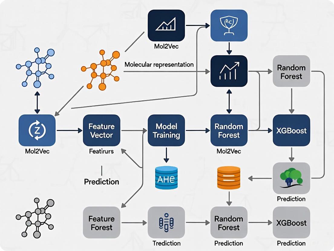
Workflow Visualization
The following diagram illustrates the integrated pipeline for molecular property prediction, highlighting the key steps from data preparation to model deployment, including the critical data consistency check.
The translation of molecular structures into information-rich numerical representations is a cornerstone of modern chemoinformatics and a critical step for harnessing machine learning in drug discovery and materials science [9]. Molecular representation learning has emerged as a powerful paradigm, moving beyond handcrafted descriptors to automatically learn salient features from molecular data [1]. Effective molecular representation bridges the gap between chemical structures and their biological, chemical, or physical properties, enabling various drug discovery tasks including virtual screening, activity prediction, and scaffold hopping [1]. These techniques allow researchers to efficiently navigate the vast chemical space and prioritize compounds with therapeutic potential, significantly accelerating the early stages of drug development [10] [1].
Classical Molecular Representation Methods
Molecular Descriptors and Fingerprints
Traditional molecular representation methods rely on explicit, rule-based feature extraction techniques, exemplified by molecular descriptors and fingerprints [1]. Molecular descriptors quantify physical or chemical properties of molecules, while fingerprints typically encode substructural information as binary strings or numerical values [1].
Molecular fingerprints are feature extraction methods based on identifying small subgraphs within a molecule and detecting their presence or counting their occurrences, yielding binary and count variants, respectively [9]. They can be broadly classified into substructural and hashed types. Substructural fingerprints detect predefined patterns determined by expert chemists, while hashed fingerprints define general shapes of extracted subgraphs and convert them into numerical identifiers using a modulo function into a fixed-length output vector [9].
Table 1: Common Molecular Fingerprint Types and Their Characteristics
| Fingerprint Type | Description | Key Features | Common Uses |
|---|---|---|---|
| Extended Connectivity Fingerprint (ECFP) | Circular neighborhoods capturing atom environments [9] | Daylight-like features, radius-dependent | Similarity searching, QSAR [1] |
| Topological Torsion (TT) | Paths of length 4 in the molecular graph [9] | Linear sequences of atoms and bonds | Molecular similarity, virtual screening |
| Atom Pair (AP) | Shortest paths between atom pairs [9] | Atom-type and distance information | Similarity searching, clustering |
Although not task-adaptive, hashed fingerprints remain widely used in chemoinformatics and molecular machine learning due to their flexibility, computational efficiency, and consistently strong performance [9]. In many cases, they continue to outperform more complex approaches, such as Graph Neural Networks (GNNs) [9].
String-Based Representations
The Simplified Molecular Input Line Entry System (SMILES) provides a compact and efficient way to encode chemical structures as strings and has become a widely used method for molecular representation [1]. Despite its simplicity and convenience, SMILES has inherent limitations in capturing the full complexity of molecular interactions [1]. As drug discovery tasks grow more sophisticated, traditional string-based representations often fall short in reflecting the intricate relationships between molecular structure and key drug-related characteristics such as biological activity and physicochemical properties [1].
Modern AI-Driven Embedding Approaches
Graph-Based Neural Representations
Graph neural networks offer a natural framework for molecular representation since molecules are inherently graph-structured with atoms as nodes and bonds as edges [9]. Most GNN architectures follow a message-passing framework where initial atom embeddings consist of elementary chemical descriptors, and in each GNN layer, atoms receive embeddings from their neighbors and update their own embedding accordingly [9]. To obtain a whole-molecule embedding, atom embeddings are aggregated using a readout function such as channel-wise average or sum [9].
The Graph Isomorphism Network (GIN) is one of the most widely used GNN architectures, as it was proven to be as expressive as the Weisfeiler-Lehman isomorphism test in distinguishing non-isomorphic graphs [9]. Recent advancements include models like ChemXTree, a feature-enhanced GNN framework that integrates a Gate Modulation Feature Unit and neural decision tree in the output layer to improve predictive accuracy for drug discovery tasks [11].
Language Model-Based Approaches
Inspired by advances in natural language processing, transformer models have been adapted for molecular representation by treating molecular sequences as a specialized chemical language [1]. Unlike traditional methods like ECFP fingerprints that encode predefined substructures, this approach tokenizes molecular strings at the atomic or substructure level [1]. Each token is mapped into a continuous vector, and these vectors are then processed by architectures like Transformers or BERT [1].
The Mol2Vec Approach
Mol2Vec is an unsupervised machine learning approach to learn vector representations of molecular substructures, inspired by natural language processing techniques like Word2vec [12]. Similar to how Word2vec models place vectors of closely related words in close proximity in the vector space, Mol2vec learns vector representations of molecular substructures that point in similar directions for chemically related substructures [12].
Compounds can be encoded as vectors by summing the vectors of the individual substructures, and these representations can be fed into supervised machine learning approaches to predict compound properties [12]. The resulting Mol2vec model is pretrained once, yields dense vector representations, and overcomes drawbacks of common compound feature representations such as sparseness and bit collisions [12].
Experimental Protocols and Implementation
Protocol: Generating Mol2Vec Embeddings
Objective: Generate continuous vector representations for molecules using the Mol2Vec approach.
Materials:
- Chemical compound dataset in SMILES format
- Mol2Vec pretrained model
- RDKit or similar cheminformatics toolkit
- Python environment with mol2vec library
Procedure:
- Data Preparation:
- Convert SMILES strings to RDKit molecule objects
- Standardize molecules (neutralization, tautomer removal)
- Curate dataset to remove duplicates and invalid structures
Substructure Identification:
- Apply Morgan circular fingerprints with radius 1-2
- Extract molecular substructures using the RDKit Morgan algorithm
- Create a "sentence" representation for each molecule where "words" are substructure identifiers
Model Training:
- Initialize the Word2Vec model with desired dimensions (typically 100-300)
- Set window size based on molecular complexity (typically 10-20)
- Train on the corpus of molecular "sentences" for multiple epochs
- Save the pretrained substructure embeddings
Molecular Vector Generation:
- For new molecules, identify substructures using the same procedure
- Retrieve corresponding vectors from the pretrained model
- Sum all substructure vectors to obtain the molecular embedding
Validation:
- Assess embedding quality using similarity search for known similar compounds
- Evaluate performance on benchmark tasks like molecular property prediction
- Compare with traditional fingerprints for well-established structure-activity relationships
Protocol: Molecular Property Prediction with Tree-Based Models
Objective: Predict molecular properties using Mol2Vec embeddings with tree-based ensemble models.
Materials:
- Molecular embeddings (from Protocol 4.1)
- Property annotation data
- LightGBM or XGBoost libraries
- Scikit-learn for model evaluation
Procedure:
- Feature Preparation:
- Split data into training, validation, and test sets (e.g., 70/15/15)
- Standardize features if necessary for the specific tree implementation
- Address class imbalance through weighting or sampling techniques
Model Training:
- Initialize LightGBM or XGBoost classifier/regressor
- Set hyperparameters (learning rate, max depth, number of estimators)
- Use cross-validation to optimize hyperparameters
- Train multiple random seeds for robustness assessment
Model Evaluation:
- Predict on held-out test set
- Calculate performance metrics: ROC-AUC, accuracy, precision, recall
- Compare with baseline models (random forest, SVM, neural networks)
- Perform statistical significance testing on performance differences
Model Interpretation:
- Analyze feature importance scores
- Apply SHAP analysis to understand embedding contribution
- Identify key substructures driving predictions
Performance Benchmarking and Applications
Comparative Performance of Representation Methods
Recent comprehensive benchmarking studies have evaluated numerous molecular representation approaches across multiple datasets and tasks. Surprisingly, many sophisticated neural models show negligible or no improvement over traditional molecular fingerprints, with only specialized fingerprint-based models demonstrating statistically significant advantages [9].
Table 2: Performance Comparison of Molecular Representation Methods on Benchmark Tasks
| Representation Method | BBBP (ROC-AUC) | BACE (ROC-AUC) | HIV (ROC-AUC) | ClinTox (ROC-AUC) |
|---|---|---|---|---|
| ECFP Fingerprints | Baseline | Baseline | Baseline | Baseline |
| D-MPNN | 71.0 (0.3) | 80.9 (0.6) | 77.1 (0.5) | 90.6 (0.6) |
| Attentive FP | 64.3 (1.8) | 78.4 (0.02) | 75.7 (1.4) | 84.7 (0.3) |
| N-Gram RF | 69.7 (0.6) | 77.9 (1.5) | 77.2 (0.1) | 77.5 (4.0) |
| PretrainGNN | 68.7 (1.3) | 84.5 (0.7) | 79.9 (0.7) | 72.6 (1.5) |
| GROVERbase | 70.0 (0.1) | 82.6 (0.7) | 62.5 (0.0) | N/A |
| ChemXTree | ~76.0* | ~86.0* | ~78.0* | ~91.0* |
Note: Values for ChemXTree are approximate based on reported improvements in [11]. Standard deviations shown in parentheses where available.
Application in Anticancer Ligand Prediction
The ACLPred framework demonstrates a successful application of molecular representation with tree-based models for predicting anticancer ligands [10]. Using Light Gradient Boosting Machine with molecular descriptors, ACLPred achieved prediction accuracy of 90.33% with AUROC of 97.31% on independent test data [10].
Key aspects of this implementation include:
- Feature Selection: Multistep feature selection with variance threshold, correlation filter, and Boruta algorithm to identify significant molecular descriptors [10]
- Model Architecture: LightGBM classifier optimized through hyperparameter tuning and cross-validation [10]
- Interpretability: SHAP analysis revealed that topological features made major contributions to decision-making, providing model interpretability [10]
Table 3: Key Research Reagent Solutions for Molecular Embedding Experiments
| Resource | Type | Function | Implementation Example |
|---|---|---|---|
| RDKit | Cheminformatics Library | Molecular manipulation, descriptor calculation, fingerprint generation | Convert SMILES to molecular graphs, calculate molecular descriptors [10] |
| PaDELPy | Descriptor Calculation | Compute molecular descriptors and fingerprints | Generate 1D/2D molecular descriptors for feature engineering [10] |
| LightGBM | Machine Learning Library | Gradient boosting framework for tabular data | Build predictive models for molecular property prediction [10] |
| Mol2Vec | Embedding Algorithm | Generate continuous vector representations of molecules | Create unsupervised molecular embeddings for downstream tasks [12] |
| SHAP | Interpretation Framework | Explain machine learning model predictions | Interpret tree-based model decisions and identify important features [10] |
| MoleculeNet | Benchmark Suite | Standardized datasets for molecular machine learning | Evaluate model performance across multiple tasks [11] |
Molecular embedding techniques represent a critical advancement in computational chemistry and drug discovery, enabling the translation of chemical structures into machine-readable vectors. While traditional fingerprints like ECFP remain surprisingly competitive, modern approaches like Mol2Vec and graph neural networks offer complementary advantages for specific applications [9]. The integration of these representations with powerful tree-based models creates a robust pipeline for molecular property prediction, as demonstrated by frameworks like ACLPred for anticancer ligand prediction [10]. As the field evolves, the optimal approach likely involves selecting representation methods based on specific task requirements, data availability, and interpretability needs, with hybrid methods showing particular promise for addressing the complex challenges in computational drug discovery.
Mol2Vec is an unsupervised machine learning approach that generates continuous vector representations of molecular substructures, drawing direct inspiration from Natural Language Processing (NLP) techniques. The fundamental analogy at the heart of Mol2Vec is to consider a molecule as a "sentence" and its constituent substructures as "words." This conceptual framework allows the application of the powerful Word2vec algorithm to the chemical domain, enabling the embedding of chemical intuition into a high-dimensional vector space. By training on a large corpus of molecules, the model learns to position chemically similar substructures close to one another in a 300-dimensional space, effectively capturing latent structure-property relationships without the need for supervised labeling. This methodology represents a paradigm shift from traditional binary fingerprints to continuous, information-rich vector representations that have demonstrated state-of-the-art performance for both classification and regression tasks in molecular property prediction [13] [14].
The core innovation of Mol2Vec lies in its ability to capture the context of molecular substructures much like Word2vec captures semantic meaning in language. Just as the word "king" is spatially related to "man" and "queen" in the vector space of Word2vec, chemically related functional groups and substructures exhibit specific spatial relationships in the Mol2vec embedding space. This capability to encode chemical similarity and relationships in a continuous space provides a rich foundation for building predictive models in cheminformatics and drug discovery [13].
How Mol2Vec Works: From Molecules to Vector Embeddings
The Mol2Vec Pipeline: A Step-by-Step Protocol
The process of generating Mol2Vec embeddings follows a systematic pipeline that transforms raw molecular structures into meaningful vector representations. The following workflow illustrates this complete process:
Step 1: Corpus Preparation The process begins with assembling a large and chemically diverse corpus of molecules from databases such as ChEMBL (containing bioactivity data) and ZINC (containing commercially available compounds). The original Mol2Vec publication utilized approximately 19.9 million molecules from these sources. Each molecule is converted into its canonical SMILES representation using RDKit, ensuring a standardized molecular representation [13].
Step 2: Substructure Identification Using Morgan Fingerprints For each molecule in the corpus, all substructures contributing to a Morgan fingerprint with a radius of one are extracted. The Morgan algorithm generates atom identifiers that represent specific circular substructures around each atom, effectively breaking down each molecule into its fundamental structural components. These identifiers serve as the "words" that form the molecular "sentence" and have the same order as the canonical SMILES representation [13] [15].
Step 3: Word2Vec Model Training The collection of molecular "sentences" is used to train a Word2Vec model, specifically using the Skip-gram architecture with a window size of 10 and 300-dimensional embeddings. The Skip-gram model was selected as it better captures spatial relationships through its weighting of context words. During training, rare substructures occurring less than three times in the corpus are replaced with an "UNSEEN" token, which typically learns a vector close to zero [13] [15].
Step 4: Molecular Vector Generation To represent an entire molecule as a single vector, all substructure vectors for that molecule are summed together. If an unknown identifier is encountered during featurization of new data, the "UNSEEN" vector is employed. This additive approach preserves information about all substructures present in the molecule while generating a fixed-length representation regardless of molecular size [15].
Key Research Reagents and Computational Tools
Table 1: Essential Research Reagents and Software for Mol2Vec Implementation
| Resource Name | Type | Function/Purpose | Source/Reference |
|---|---|---|---|
| RDKit | Cheminformatics Library | Converts molecules to canonical SMILES; generates Morgan fingerprints for substructure extraction | [13] [16] |
| Gensim | NLP Library | Implements Word2Vec algorithm for training substructure embeddings | [13] |
| ChEMBL Database | Chemical Database | Provides bioactivity data for ~19.9 million molecules for corpus building | [13] |
| ZINC Database | Chemical Database | Supplies commercially available compounds to diversify training corpus | [13] |
| Mol2Vec Python Package | Specialized Library | Offers implemented Mol2Vec methodology for generating molecular vectors | [17] |
| Scikit-learn | Machine Learning Library | Provides Random Forest and other ML algorithms for property prediction | [13] |
| XGBoost/LightGBM | Gradient Boosting Frameworks | Ensemble methods for regression and classification tasks | [18] [16] |
Performance Benchmarking and Experimental Validation
Quantitative Assessment Across Diverse Molecular Properties
Extensive validation studies have demonstrated Mol2Vec's performance across various molecular property prediction tasks. The following table summarizes key benchmarking results from multiple studies:
Table 2: Performance Benchmarking of Mol2Vec Embeddings Across Various Tasks
| Dataset/Property | Task Type | Model Architecture | Performance Metrics | Comparative Performance |
|---|---|---|---|---|
| ESOL (Solubility) | Regression | GBM with Mol2Vec | R²cv = 0.86 | Superior to Morgan FP-GBM (R²cv = 0.66) [13] |
| Ames Mutagenicity | Classification | RF with Mol2Vec | State-of-the-art AUC | Recommended architecture for classification [13] |
| Tox21 | Classification | RF with Mol2Vec | State-of-the-art AUC | Outperformed SVM, NBC, CNN on toxicity targets [13] |
| Kinase Specificity | Proteochemometrics | PCM with Mol2Vec | High accuracy in cross-validation | Effective for unknown compound-target pairs [13] |
| Polymer Properties | Regression | ML with Mol2Vec | Improved accuracy | Effective even with small datasets (n=214) [19] |
| Critical Temperature | Regression | GBR with Mol2Vec | R² = 0.93 | Slightly higher accuracy than VICGAE embeddings [16] |
| Lipophilicity | Regression | GBFS with Mol2Vec | Superior performance | Outperformed state-of-the-art benchmarks [18] |
The table demonstrates that Mol2Vec embeddings consistently deliver competitive or superior performance compared to traditional molecular representations like Morgan fingerprints and other state-of-the-art algorithms. Notably, the combination of Mol2Vec with tree-based methods like Random Forest (for classification) and Gradient Boosting Machines (for regression) appears particularly effective across diverse chemical tasks [13] [18].
Comparative Analysis of Embedding Approaches
The performance of Mol2Vec must be understood in the context of alternative molecular representation approaches. The following diagram compares the key characteristics of different representation methods:
Mol2Vec offers distinct advantages over traditional fingerprints: (1) Lower dimensionality (300 dimensions vs. 2048-4096 bits for Morgan fingerprints) reduces memory requirements and training time; (2) Continuous representations capture nuanced similarity relationships beyond binary presence/absence; (3) Chemical intuition emerges through the spatial arrangement of related substructures in the embedding space [13] [20]. Compared to other learned representations like Graph Neural Networks (GNNs) or transformer models (e.g., MOLFORMER), Mol2Vec provides a favorable balance between predictive accuracy and computational requirements, making it particularly suitable for research environments with limited computational resources [18] [16].
Application Notes and Protocols for Molecular Property Prediction
Protocol: Building a Molecular Property Prediction Pipeline with Mol2Vec and Tree-Based Models
This protocol details the complete workflow for predicting molecular properties using Mol2Vec embeddings combined with tree-based ensemble methods, specifically designed for integration into a broader thesis research framework on molecular property prediction pipelines.
Step 1: Data Preparation and Preprocessing
- Input: Collect SMILES strings of target molecules and their corresponding property values (experimental or computational)
- Preprocessing: Standardize SMILES representations using RDKit's CanonSmiles function
- Data Splitting: Implement appropriate cross-validation splits based on research question:
- Random Split: Standard validation for generalizability
- Scaffold Split: Tests performance on novel molecular scaffolds
- Temporal Split: Mimics real-world discovery scenarios
Step 2: Mol2Vec Embedding Generation
- Load Pretrained Model: Utilize the pretrained Mol2Vec model (300 dimensions, trained on ZINC and ChEMBL)
- Generate Molecular Vectors:
- Handle Unknown Substructures: Replace vectors for unrecognized substructures with the "UNSEEN" vector
Step 3: Feature Selection and Engineering (Optional but Recommended)
- Gradient-Boosted Feature Selection (GBFS): Implement correlation analysis and importance weighting to identify the most relevant dimensions for the target property
- Dimensionality Reduction: For very small datasets (<500 molecules), consider PCA or UMAP to reduce dimensionality while preserving variance
Step 4: Model Training and Hyperparameter Optimization
- Algorithm Selection:
- For classification tasks (e.g., mutagenicity, toxicity): Use Random Forest with balanced class weights
- For regression tasks (e.g., solubility, lipophilicity): Use Gradient Boosting Machines (XGBoost, LightGBM, CatBoost)
- Hyperparameter Tuning:
- Random Forest: Optimize number of trees (100-1000), maximum depth (3-20), and minimum samples per leaf (1-5)
- Gradient Boosting: Optimize learning rate (0.01-0.3), number of estimators (100-2000), and maximum depth (3-8)
- Validation: Implement nested cross-validation to avoid overfitting and obtain robust performance estimates
Step 5: Model Interpretation and Validation
- Feature Importance: Analyze which embedding dimensions contribute most to predictions
- Chemical Interpretation: Project molecules into 2D space using UMAP or t-SNE to identify clusters of compounds with similar properties
- External Validation: Test model on completely held-out datasets to assess generalizability
Case Study: Predicting Aqueous Solubility (ESOL Dataset)
The ESOL (Estimated Solubility) dataset provides an excellent benchmark for demonstrating Mol2Vec's capabilities in regression tasks. The protocol for this specific application follows the general workflow but with these specific parameters:
- Dataset: 1,144 compounds with experimental aqueous solubility values [13]
- Mol2Vec Parameters: 300-dimensional embeddings generated from pretrained model
- Model: Gradient Boosting Machine (GBM) with 2000 estimators, maximum tree depth of 3, and learning rate of 0.1
- Performance: Achieved R²cv value of 0.86, significantly outperforming Morgan fingerprint-based GBM models (R²cv = 0.66) [13]
The superior performance on this dataset highlights Mol2Vec's particular advantage in low-data scenarios, where the pre-trained embeddings effectively transfer chemical knowledge learned from larger molecular corpora.
Advanced Applications and Integration Strategies
Proteochemometric Modeling with Mol2Vec and ProtVec
Mol2Vec embeddings can be combined with ProtVec vectors (which apply the same Word2vec concept to protein sequences) to create powerful proteochemometric (PCM) models that predict compound-target interactions. This integration enables the modeling of interactions between small molecules and their protein targets without requiring sequence alignments, making it particularly valuable for proteins with low sequence similarity to well-characterized targets [13] [14].
The PCM modeling approach employs specialized cross-validation strategies to assess different aspects of model performance:
- CV1: Tests performance on unknown compound-target pairs (easiest scenario)
- CV2: Tests performance on new targets by leaving out entire targets during training
- CV3: Tests performance on unknown compounds
- CV4: Tests performance on both unknown compounds and new targets (most challenging) [13]
For PCM tasks, Mol2Vec combined with Random Forest classification is specifically recommended based on rigorous validation across kinase specificity datasets [13].
Integration with Feature Selection Workflows
Recent research demonstrates that combining Mol2Vec with sophisticated feature selection methods further enhances performance while maintaining computational efficiency. The Gradient-Boosted Feature Selection (GBFS) workflow integrates Mol2Vec embeddings with statistical analysis and multicollinearity mitigation strategies to identify the most relevant substructure features for specific property prediction tasks [18].
This approach has shown particular promise for predicting quantum mechanical properties (e.g., using the QM9 dataset) and experimentally-measured physicochemical properties like lipophilicity. The feature selection process not only improves model performance but also enhances interpretability by identifying which specific substructural elements contribute most significantly to the target property [18].
Mol2Vec represents a significant advancement in molecular representation learning, effectively bridging the gap between traditional cheminformatics and modern natural language processing techniques. Its ability to capture complex structural and chemical relationships in a continuous 300-dimensional space has been rigorously validated across diverse molecular property prediction tasks, from aqueous solubility and toxicity to kinase specificity and polymer properties.
The combination of Mol2Vec embeddings with tree-based ensemble methods like Random Forest and Gradient Boosting Machines provides a particularly powerful and computationally efficient approach for molecular property prediction pipelines. This methodology demonstrates competitive or superior performance compared to more computationally intensive approaches like graph neural networks or transformer models, while offering advantages in model interpretability and resource requirements.
For researchers implementing molecular property prediction pipelines, Mol2Vec offers a robust foundation that balances chemical intuition, predictive accuracy, and computational efficiency. As the field advances, the integration of Mol2Vec with more sophisticated feature selection methods and its application to emerging areas like polymer informatics and proteochemometric modeling continue to expand its utility in accelerating drug discovery and materials design.
Molecular property prediction is a critical task in cheminformatics and drug discovery, aiming to link molecular structures with experimentally measurable biological activities or physicochemical properties [21]. In this context, tree-based ensemble models—particularly gradient boosting frameworks like XGBoost, LightGBM, and CatBoost—have emerged as powerhouse algorithms that consistently deliver state-of-the-art performance on tabular molecular data [21] [22]. Their robustness, predictive accuracy, and computational efficiency make them particularly well-suited for handling the unique challenges presented by cheminformatics datasets, which often feature high dimensionality, significant class imbalance, and potential measurement noise [21].
These algorithms excel at learning complex structure-activity relationships from molecular descriptors or embeddings, enabling researchers to build predictive models for applications ranging from virtual screening and toxicity prediction to drug sensitivity analysis [21] [16]. By leveraging ensemble techniques that combine multiple weak learners (decision trees), these methods effectively capture nonlinear relationships in molecular data while resisting overfitting through advanced regularization techniques [21] [23]. This application note explores the technical foundations of these algorithms, provides performance comparisons specific to molecular data, and outlines detailed experimental protocols for their implementation in molecular property prediction pipelines.
Algorithm Comparative Analysis
Key Characteristics and Performance
The three dominant gradient boosting implementations share a common foundation but incorporate distinct architectural innovations that yield different performance characteristics across various molecular datasets.
Table 1: Comparative Analysis of Gradient Boosting Algorithms for Molecular Data
| Feature | XGBoost | LightGBM | CatBoost |
|---|---|---|---|
| Tree Structure | Level-wise (depth-first) tree growth [21] | Leaf-wise tree growth with depth limitation [21] [23] | Symmetric (oblivious) trees with same splits per level [21] [24] |
| Handling Categorical Features | Requires extensive preprocessing/encoding [23] [24] | Optimized handling but may require encoding [23] | Native handling without preprocessing [23] [24] |
| Training Efficiency | Moderate training speed [21] [23] | Fastest training, especially on large datasets [21] [22] [23] | Competitive training speed [23] |
| Regularization Approach | L1/L2 regularization [21] [23] | Gradient-based One-Side Sampling (GOSS) [21] [23] | Ordered boosting, symmetric trees [21] [24] |
| Molecular Property Prediction Performance | Best overall predictive performance in QSAR benchmarks [21] | Excellent performance with significantly faster training times [21] | Competitive performance, excels with categorical features [25] [16] |
| Ideal Use Cases | General QSAR modeling when accuracy is priority [21] | Large-scale virtual screening, high-throughput datasets [21] [22] | Datasets with mixed feature types, smaller datasets [21] [24] |
XGBoost employs regularized learning with L1 and L2 regularization to prevent overfitting, making it particularly robust for molecular datasets where generalization is crucial [21] [23]. Its Newton descent optimization approach contributes to faster convergence compared to traditional gradient descent [21]. For molecular data, XGBoost has demonstrated superior predictive performance in comprehensive QSAR benchmarks encompassing 157,590 models across 16 datasets and 94 endpoints [21].
LightGBM introduces several efficiency optimizations including Gradient-based One-Side Sampling (GOSS) which retains instances with larger gradients while randomly sampling those with smaller gradients, and Exclusive Feature Bundling (EFB) which combines mutually exclusive features to reduce dimensionality [21] [23]. These innovations make it exceptionally efficient for large molecular datasets such as high-throughput screening data, where it can significantly reduce training time without substantial accuracy loss [21].
CatBoost's distinctive approach includes ordered boosting which prevents target leakage and overfitting by using a permutation-driven training scheme, and symmetric tree structures that serve as an implicit regularization mechanism [21] [24]. While categorical features are less common in traditional molecular descriptors [21], CatBoost's robust handling of mixed data types and strong performance on smaller datasets makes it valuable for specialized molecular prediction tasks [25] [16].
Molecular Data Performance Benchmarks
Comprehensive benchmarking studies provide empirical evidence for algorithm selection in molecular property prediction pipelines.
Table 2: Performance Benchmarks on Molecular and Materials Datasets
| Dataset Domain | Best Performing Algorithm | Key Metric | Performance Notes |
|---|---|---|---|
| QSAR (94 endpoints, 1.4M compounds) | XGBoost [21] | Predictive Accuracy | Overall best performance across diverse endpoints [21] |
| Concrete Compressive Strength (Multiple datasets) | CatBoost [25] | R²: 0.92-0.95 | Exceptional inter-dataset stability and generalization [25] |
| Molecular Properties (CRC Handbook) | Multiple [16] | R² up to 0.93 | All gradient boosting variants performed well with Mol2Vec embeddings [16] |
| Large-scale QSAR | LightGBM [21] | Training Time | Fastest training, especially beneficial for large datasets [21] |
| Critical Temperature Prediction | All Boosted Models [16] | R² = 0.93 | Excellent performance with Mol2Vec embeddings [16] |
In large-scale QSAR benchmarking encompassing 1.4 million compounds, XGBoost achieved the best overall predictive performance, while LightGBM required the least training time, particularly for larger datasets [21]. This comprehensive analysis demonstrated that all gradient boosting implementations substantially outperformed traditional machine learning approaches for molecular property prediction tasks.
For specific molecular properties such as critical temperature and critical pressure prediction, gradient boosting models combined with Mol2Vec embeddings achieved R² values up to 0.93, demonstrating their capability to capture complex structure-property relationships [16]. The performance advantage was consistent across diverse molecular families including hydrocarbons, halogenated compounds, oxygenated species, and heterocyclic molecules [16].
Experimental Protocols
Molecular Property Prediction with Gradient Boosting and Mol2Vec Embeddings
Purpose: To predict molecular properties (e.g., bioactivity, solubility, toxicity) using Mol2Vec molecular embeddings combined with gradient boosting algorithms.
Background: Mol2Vec generates unsupervised vector representations of molecular substructures, creating meaningful embeddings that capture chemical similarity [18] [16]. When combined with gradient boosting models, these embeddings enable accurate prediction of molecular properties without requiring extensive feature engineering.
Materials and Reagents:
- Chemical Compounds: Dataset of molecules with associated property measurements
- Computational Resources: Workstation or cluster with adequate RAM and CPU resources
- Software: Python environment with RDKit, gensim (Mol2Vec), and gradient boosting libraries (XGBoost, LightGBM, CatBoost)
Table 3: Research Reagent Solutions for Molecular Property Prediction
| Reagent/Resource | Specification | Function/Purpose |
|---|---|---|
| RDKit | Version 2022.09.5 or later [26] | Cheminformatics toolkit for molecule handling and descriptor calculation |
| Mol2Vec Implementation | Python implementation from original paper [16] | Generation of molecular embeddings from SMILES strings |
| Gradient Boosting Libraries | XGBoost 1.5+, LightGBM 3.3+, CatBoost 1.0+ [16] | Implementation of tree-based ensemble algorithms for model training |
| Chemical Datasets | Curated datasets from ChEMBL, TDC, or MoleculeNet [21] [26] | Standardized benchmarks for model training and validation |
| Optuna Hyperparameter Optimization | Version 2.10+ [16] | Automated hyperparameter tuning for optimal model performance |
Procedure:
Data Preparation and Preprocessing
- Obtain molecular structures in SMILES format and corresponding property values
- Curate dataset to remove duplicates and correct obvious errors
- Apply appropriate data splitting techniques (scaffold split for generalizability) [26]
- Standardize molecular structures using RDKit (normalization, tautomer standardization)
Molecular Embedding Generation
- Generate Mol2Vec embeddings for all compounds in the dataset
- Utilize the pre-trained Mol2Vec model or train a custom model on relevant chemical space
- Validate embedding quality through chemical similarity analysis and visualization
Model Training and Hyperparameter Optimization
- Implement multiple gradient boosting algorithms (XGBoost, LightGBM, CatBoost)
- Perform randomized or Bayesian hyperparameter optimization
- Employ nested cross-validation to ensure robust performance estimation
- Monitor training with appropriate validation metrics to prevent overfitting
Model Evaluation and Interpretation
- Evaluate final models on held-out test set using multiple metrics (RMSE, R², etc.)
- Analyze feature importance to identify influential molecular substructures
- Apply SHAP analysis for model interpretability and mechanistic insights [24]
Troubleshooting:
- Poor performance may indicate inadequate chemical space coverage in training data
- Overfitting can be addressed through increased regularization or ensemble simplification
- Training instability may require learning rate reduction or different tree growth strategies
Comprehensive Benchmarking Protocol for Algorithm Selection
Purpose: To systematically compare gradient boosting algorithms for specific molecular prediction tasks and identify the optimal approach.
Procedure:
Dataset Characterization
- Analyze dataset size, feature dimensionality, and class distribution
- Assess dataset balance and identify potential biases
- Perform chemical space analysis to understand structural diversity
Standardized Implementation
- Implement all algorithms with consistent preprocessing and evaluation frameworks
- Use identical cross-validation splits for fair comparison
- Apply comparable hyperparameter optimization effort to each algorithm
Multi-dimensional Evaluation
- Assess predictive performance using task-appropriate metrics
- Evaluate computational efficiency (training time, inference speed)
- Analyze model robustness and stability across multiple runs
- Consider model interpretability and feature importance consistency
Optimal Algorithm Selection
- Select algorithm based on project priorities (accuracy vs. speed vs. interpretability)
- Document performance characteristics for future reference
- Establish implementation best practices for selected algorithm
Implementation Guidelines
Algorithm Selection Framework
Choosing the appropriate gradient boosting algorithm depends on specific dataset characteristics and project requirements. The following decision framework provides guidance for algorithm selection:
Critical Implementation Considerations
Hyperparameter Optimization: Extensive hyperparameter tuning is crucial for maximizing predictive performance. Key hyperparameters include learning rate, tree depth, regularization terms, and subsampling ratios [21]. Automated optimization frameworks like Optuna [16] or RandomizedSearchCV can systematically explore the hyperparameter space.
Data Consistency Assessment: Before model training, rigorously assess data quality and consistency, particularly when integrating datasets from multiple sources. Tools like AssayInspector can identify distributional misalignments, outliers, and batch effects that could compromise model performance [26].
Feature Importance Interpretation: While all gradient boosting algorithms provide feature importance metrics, these should be interpreted with caution as different algorithms may rank molecular features differently due to variations in regularization and tree structures [21]. Expert chemical knowledge should always complement data-driven interpretations.
Molecular Representations: The choice of molecular representation significantly impacts model performance. While this protocol focuses on Mol2Vec embeddings, alternative representations including ECFP fingerprints, traditional molecular descriptors, or learned representations from graph neural networks may be preferable for specific applications [16] [26].
XGBoost, LightGBM, and CatBoost represent the state-of-the-art in tree-based ensemble learning for molecular property prediction, each offering distinct advantages for different scenarios within the drug discovery pipeline. XGBoost generally achieves the highest predictive accuracy, LightGBM offers exceptional computational efficiency for large-scale screening applications, and CatBoost provides robust performance with minimal preprocessing requirements. By implementing the standardized protocols and decision frameworks outlined in this application note, researchers can systematically leverage these powerful algorithms to accelerate molecular design and optimization campaigns. The integration of these methods with modern molecular representations like Mol2Vec creates a robust foundation for predictive modeling in cheminformatics, ultimately contributing to more efficient drug discovery processes.
The prediction of molecular properties such as melting point (MP), boiling point (BP), toxicity, and bioactivity constitutes a critical foundation in chemical research and drug discovery. These properties determine the behavior, efficacy, and safety profiles of chemical compounds, influencing their application in pharmaceuticals, materials science, and industrial chemistry. Accurate prediction of these properties enables researchers to screen compounds virtually, significantly reducing the reliance on time-consuming and resource-intensive experimental methods [27] [16]. The advent of artificial intelligence (AI) and machine learning (ML) has revolutionized this field, shifting the paradigm from experience-driven to data-driven evaluation [27]. This document outlines detailed application notes and protocols for assessing these key molecular properties, framed within a research context focused on building molecular property prediction pipelines using Mol2Vec embeddings and tree-based models.
Key Molecular Properties and Determining Factors
Melting Point and Boiling Point
Melting point is the temperature at which a substance transitions from solid to liquid, while boiling point is the temperature at which its vapor pressure equals the surrounding atmospheric pressure [28]. Both are colligative properties strongly influenced by the strength of intermolecular forces between molecules.
Primary Determining Factors:
- Intermolecular Forces: The relative strength of cohesive intermolecular interactions follows this general order: Ionic > Hydrogen bonding > Dipole-dipole > Van der Waals dispersion forces [29] [28] [30]. Molecules with functional groups capable of stronger interactions typically exhibit higher melting and boiling points.
- Molecular Weight and Surface Area: For molecules with similar functional groups, boiling points increase with molecular weight and surface area. Larger molecules with greater surface areas can form more intermolecular interactions [29] [30].
- Molecular Symmetry and Branching: Symmetrical molecules pack more efficiently in solid crystal structures, leading to higher melting points [28]. In contrast, branching tends to decrease boiling points by reducing molecular surface area and thus weakening Van der Waals dispersion forces [30].
Table 1: Factors Affecting Melting and Boiling Points of Organic Compounds
| Factor | Effect on Boiling Point | Effect on Melting Point | Example Comparison |
|---|---|---|---|
| Intermolecular Forces | Increases with stronger forces | Increases with stronger forces | Butane (BP: -0.5°C) vs. 1-butanol (BP: 117°C) [30] |
| Molecular Weight | Increases with higher molecular weight | Generally increases with higher molecular weight | CH₄ (BP: -161.5°C) < C₂H₆ (BP: -88.6°C) < C₃H₈ (BP: -42°C) [31] |
| Branching | Decreases with increased branching | Variable; often increases with symmetry | Pentane (BP: 36°C) > 2,2-dimethylpropane (BP: 9.5°C) [28] [30] |
| Hydrogen Bonding | Significantly increases | Significantly increases | Dimethyl ether (BP: -24.8°C) < Ethanol (BP: 78.4°C) [31] |
Toxicity and Bioactivity
Toxicity refers to the potential of a substance to cause harm to living organisms, while bioactivity describes its effect on a living organism or tissue, encompassing both therapeutic and adverse effects [32].
Key Aspects and Endpoints:
- ADMET Profiles: Toxicity is a crucial component of the comprehensive ADMET (Absorption, Distribution, Metabolism, Excretion, and Toxicity) evaluation, which determines a drug's fate in the body and its clinical viability [27].
- Common Toxicity Endpoints: These include acute toxicity (e.g., LD₅₀), organ-specific toxicities (e.g., hepatotoxicity, cardiotoxicity, nephrotoxicity), carcinogenicity, and genotoxicity [27] [32].
- Molecular Targets: Bioactivity often involves interaction with specific biological targets like enzymes (e.g., beta-secretase in Alzheimer's disease), ion channels (e.g., hERG channel linked to cardiotoxicity), and receptors [27] [33].
Table 2: Common Toxicity Endpoints and Relevant Assays
| Toxicity Endpoint | Description | Typical Assays/Measurements |
|---|---|---|
| Acute Toxicity | Adverse effects following a single dose or short-term exposure | LD₅₀ (median lethal dose), IGC₅₀ (half-maximal inhibitory concentration) [27] |
| Hepatotoxicity | Drug-induced liver injury | Elevated ALT, AST, bilirubin levels [27] |
| Cardiotoxicity | Heart muscle damage; often linked to hERG channel inhibition | hERG channel inhibition assays [27] [32] |
| Nephrotoxicity | Kidney damage | Serum creatinine, blood urea nitrogen measurements [27] |
| Carcinogenicity | Potential to cause cancer | Long-term animal studies, in vitro mutagenicity tests [27] |
| Genotoxicity | Damage to genetic information | Ames test, chromosomal aberration assays [32] |
Computational Prediction Methodology
Molecular Representation with Mol2Vec
A fundamental challenge in computational molecular property prediction is transforming molecular structures into machine-readable numerical representations. Mol2Vec is an unsupervised machine learning approach that generates molecular embeddings by learning from representations of molecular substructures [16] [34]. It treats a molecule as a "sentence" composed of "words" (its substructures) and produces a fixed-dimensional vector that captures essential chemical and structural information, making it suitable for use with machine learning algorithms.
Tree-Based Ensemble Models
Tree-based ensemble methods have demonstrated remarkable success in capturing complex structure-property relationships in molecular data [16]. These models combine multiple decision trees to improve predictive performance and robustness.
Commonly Used Tree-Based Models:
- Gradient Boosting Regression (GBR): Builds trees sequentially, with each tree correcting errors of its predecessor.
- XGBoost: An optimized gradient boosting system known for its speed and performance [16].
- LightGBM (LGBM): A gradient boosting framework that uses tree-based learning algorithms, designed for high efficiency and low memory usage [16].
- CatBoost: A gradient boosting algorithm effective for datasets with categorical features [16].
Integrated Prediction Pipeline
The integration of Mol2Vec embeddings with tree-based models creates a powerful pipeline for molecular property prediction. The typical workflow, as implemented in platforms like ChemXploreML, involves several key stages [16] [34]:
- Data Collection and Standardization: Molecular structures are gathered from reliable sources (e.g., CRC Handbook, PubChem) and standardized using canonical SMILES representations.
- Molecular Embedding: Mol2Vec generates numerical feature vectors for each molecule.
- Model Training and Validation: Tree-based models are trained on the embedded data using cross-validation techniques to prevent overfitting.
- Performance Evaluation: Models are assessed using metrics such as R² (coefficient of determination) for regression tasks and AUC (Area Under the ROC Curve) for classification tasks.
Figure 1: Workflow of molecular property prediction pipeline using Mol2Vec and tree-based models.
Experimental Protocols
Protocol: Predicting Melting and Boiling Points with ChemXploreML
Purpose: To predict melting point (MP) and boiling point (BP) of organic compounds using a Mol2Vec and tree-based model pipeline.
Materials and Software:
- ChemXploreML desktop application [16] [34]
- Dataset of molecular structures with experimental MP/BP values (e.g., from CRC Handbook of Chemistry and Physics)
- Python environment with RDKit, scikit-learn, and Mol2Vec dependencies
Procedure:
- Data Preparation:
- Compile a dataset of organic compounds with known melting and boiling points. The dataset should include canonical SMILES representations for each compound.
- Use RDKit to validate and standardize all SMILES strings to ensure consistent molecular representation [16].
Molecular Embedding:
- Input the standardized SMILES strings into the Mol2Vec algorithm to generate 300-dimensional molecular embeddings for each compound [16] [34].
- Alternatively, consider using VICGAE (Variance-Invariance-Covariance regularized GRU Auto-Encoder) embeddings (32 dimensions) for computationally efficient processing with comparable performance [16].
Model Training:
- Split the dataset into training (70-80%), validation (10-15%), and test (10-15%) sets using scaffold splitting to ensure generalizability to novel chemical structures [16].
- Configure tree-based models (XGBoost, CatBoost, LightGBM) in ChemXploreML and train them on the Mol2Vec-embedded training data [16].
- Perform hyperparameter optimization using frameworks like Optuna to maximize model performance [16].
Validation and Prediction:
- Evaluate model performance on the test set using R² values and root-mean-square error (RMSE).
- For reference, established pipelines have achieved R² values up to 0.93 for well-distributed properties like critical temperature [16] [34].
- Use the trained model to predict MP/BP for new compounds of interest.
Protocol: Assessing Toxicity and Bioactivity with AI Models
Purpose: To predict toxicity endpoints and bioactivity of candidate compounds using advanced AI frameworks.
Materials and Software:
- Toxicity databases (e.g., Tox21, ClinTox, hERG Central) [32]
- AI prediction platforms (e.g., ImageMol, DLF-MFF) [33] [35]
- Molecular descriptor calculation tools (e.g., RDKit)
Procedure:
- Data Collection and Preprocessing:
- Curate a dataset of compounds with known toxicity endpoints or bioactivity profiles from public databases like Tox21 (8,249 compounds across 12 toxicity targets) or hERG Central (300,000+ records of hERG channel inhibition) [32].
- Standardize molecular structures and calculate relevant molecular descriptors (e.g., molecular weight, logP, topological polar surface area) [32].
Model Selection and Training:
- For comprehensive molecular representation, consider multi-feature fusion models like DLF-MFF that integrate molecular fingerprints, 2D/3D molecular graphs, and molecular images [35].
- Implement appropriate data splitting strategies (e.g., scaffold split) to evaluate model generalizability to structurally novel compounds [33].
- For classification tasks (e.g., toxic vs. non-toxic), use tree-based classifiers or deep learning models trained on molecular representations.
Performance Evaluation:
- Assess classification models using AUC (Area Under the ROC Curve), with state-of-the-art models like ImageMol achieving AUC values of 0.847-0.975 on benchmark toxicity datasets [33].
- For regression tasks (predicting continuous values like IC₅₀), use RMSE (Root Mean Square Error) and R² values.
- Apply interpretability techniques such as SHAP analysis to identify molecular features contributing to toxicity predictions [32].
Experimental Validation:
Table 3: Key Resources for Molecular Property Prediction Research
| Resource | Type | Function/Application |
|---|---|---|
| CRC Handbook of Chemistry and Physics | Database | Provides reliable experimental data for melting points, boiling points, and other physicochemical properties for model training and validation [16] [34] |
| RDKit | Software | Open-source cheminformatics toolkit used for SMILES standardization, molecular descriptor calculation, and fingerprint generation [16] |
| PubChem | Database | Public repository of chemical compounds and their biological activities, providing molecular structures and bioactivity data [16] |
| Tox21 | Database | Curated dataset of ~12,000 compounds tested against 12 toxicity targets across nuclear receptor and stress response pathways [33] [32] |
| Mol2Vec | Algorithm | Generates molecular embeddings from substructure representations for machine learning applications [16] [34] |
| XGBoost | Algorithm | Optimized gradient boosting tree-based model for regression and classification tasks in molecular property prediction [16] |
| Optuna | Software | Hyperparameter optimization framework for efficiently tuning machine learning models [16] |
| hERG Assay Kits | Experimental Reagent | In vitro testing systems for assessing compound binding to hERG potassium channels, predicting cardiotoxicity risk [27] [32] |
| Human Liver Microsomes | Experimental Reagent | In vitro system for evaluating metabolic stability and metabolite formation, predicting hepatic clearance and toxicity [27] |
The accurate prediction of key molecular properties including melting point, boiling point, toxicity, and bioactivity is fundamental to advancing chemical research and streamlining drug discovery. This document has outlined the theoretical foundations, computational methodologies, and detailed experimental protocols for assessing these properties, with a specific focus on pipelines utilizing Mol2Vec embeddings and tree-based models. The integration of these advanced computational approaches enables researchers to rapidly screen compound libraries, prioritize promising candidates, and identify potential toxicity liabilities early in the development process. As AI and machine learning technologies continue to evolve, molecular property prediction will become increasingly accurate and integral to the design of novel compounds with optimized characteristics for therapeutic and industrial applications.
Within a molecular property prediction pipeline utilizing Mol2Vec embeddings and tree-based models, the consistency and quality of input structural data are paramount. The performance of advanced machine learning algorithms, including Gradient Boosting Regression (GBR), XGBoost, and LightGBM (LGBM), is contingent upon the integrity of the molecular representations from which features are derived [16]. SMILES (Simplified Molecular Input Line Entry System) strings, while a universal linear notation for molecules, can exhibit significant representational variability for the same chemical compound due to factors such as tautomerism, ionization states, and disparate atom-ordering algorithms from different sources [36]. This variability introduces noise that can obscure fundamental structure-property relationships, ultimately compromising the predictive accuracy of the model.
The RDKit toolkit addresses this critical data preprocessing challenge directly. As an open-source cheminformatics library, it provides a robust set of data structures and algorithms for manipulating chemical information [37]. This application note details standardized protocols using RDKit's MolStandardize module to canonicalize and clean molecular structures, transforming raw, heterogeneous SMILES data into a consistent, standardized representation. By integrating these protocols at the outset of a Mol2Vec and tree-based model pipeline, researchers can ensure that the subsequent steps of feature generation (embedding) and model training are performed on a reliable chemical dataset, thereby enhancing the robustness and generalizability of the resulting property prediction models [16] [36].
The Scientist's Toolkit: Essential Research Reagents & Solutions
The following table catalogues the essential software tools and their specific functions within a cheminformatics pipeline focused on molecular standardization and property prediction.
Table 1: Essential Research Reagents & Solutions for Molecular Standardization and Property Prediction
| Item Name | Function/Application | Key Features / Notes |
|---|---|---|
| RDKit [37] | Core open-source toolkit for cheminformatics; used for reading molecules, structural manipulation, and descriptor calculation. | - Business-friendly BSD license- Python 3.x wrappers via Boost.Python- Provides 2D/3D molecular operations and descriptor generation for machine learning. |
| RDKit MolStandardize Module [36] [38] | Provides functions for standardizing molecular representations and normalizing functional groups. | - Includes methods for cleanup, desalting, metal disconnection, reionization, and tautomer enumeration.- Allows for definition and application of custom standardization rules. |
| Mol2Vec [12] | Generates vector representations (embeddings) of molecular substructures in an unsupervised manner. | - Inspired by Word2vec models from Natural Language Processing.- Produces a single, dense vector for an entire molecule by summing the vectors of its substructures. |
| Tree-Based Ensemble Models (e.g., LightGBM, XGBoost, CatBoost) [16] [10] | Machine learning algorithms used for the final molecular property prediction task. | - Known for handling complex, non-linear structure-property relationships.- LGBM has demonstrated high accuracy, e.g., 90.33% in anticancer ligand prediction [10]. |
| Python Scientific Stack (e.g., scikit-learn, Pandas, NumPy) [16] | Provides the computational environment for data handling, preprocessing, and model implementation. | - Essential for scripting the analysis pipeline, from data loading and RDKit processing to model training and validation. |
Application Notes: SMILES Standardization with RDKit
The Critical Role of Standardization in Prediction Pipelines
In the context of molecular property prediction, the primary objective of SMILES standardization is to represent all molecules from diverse sources in a single, consistent manner [36]. Chemical intuition suggests that different representations of the same molecule should yield identical or highly similar feature vectors. Without standardization, a single molecule represented by multiple SMILES strings could be treated as distinct entities by the Mol2Vec algorithm, leading to fragmented and unreliable feature sets. Research has shown that the choice of molecular embedding, such as Mol2Vec, significantly impacts the performance of subsequent machine learning models [16]. Standardization acts as a foundational step to mitigate this source of noise, ensuring that the learned embeddings reflect genuine chemical similarities rather than representational artifacts.
The standardization process specifically addresses several chemical challenges:
- Tautomerism: A molecule can exist as multiple tautomers, which are constitutional isomers that readily interconvert. The
TautomerEnumeratoris used to select a canonical tautomeric form [36]. - Charged States and Salts: Molecules may be represented with irrelevant counterions or in non-standard ionization states. The standardization pipeline includes steps to disconnect metals, remove salts, and neutralize molecules where appropriate [36] [38].
- Fragment Handling: Input data often contains salts or mixtures. The
FragmentParentfunction helps isolate the largest organic covalent unit, which is typically the chemical structure of interest [36].
Core Standardization Functions and Parameters
RDKit's MolStandardize module encapsulates a series of operations designed to address the challenges outlined above. The key functions and their parameters are summarized below.
Table 2: Core Functions and Parameters in RDKit's MolStandardize Module
| Function / Class | Key Parameters / Attributes | Primary Action |
|---|---|---|
Cleanup(mol) [36] |
(Convenience function, parameters internal) | Performs a composite cleanup: remove hydrogens, disconnect metal atoms, normalize functional groups, and reionize the molecule. |
FragmentParent(clean_mol) [36] |
- | Returns the largest covalent fragment in the molecule, effectively desalting and removing small organic fragments. |
Uncharger() [36] |
- | Attempts to neutralize the molecule while preserving the natural representation of zwitterions. |
TautomerEnumerator() [36] |
Canonicalize(mol) |
Applies a set of transformation rules to generate the canonical tautomer for the molecule. |
Normalizer() [38] |
normalize(mol), normalizeInPlace(mol) |
Applies a set of chemical transformations (e.g., sulfoxide normalization, nitro group normalization) to standardize functional groups. Can be initialized with custom rules. |
Experimental Protocols
Basic Molecular Standardization Workflow
This protocol describes a standard pipeline for converting a raw SMILES string into a standardized molecule, ready for the generation of Mol2Vec embeddings or other molecular descriptors.
- Input Raw SMILES. Begin with a SMILES string, for example,
'C1=CC(=C(C=C1Cl)Cl)NC(C)(C)C(=O)O'. - Convert to Molecule Object. Use
mol = Chem.MolFromSmiles(smiles)to parse the SMILES string and create an RDKit molecule object. - Initial Cleanup. Apply the
rdMolStandardize.Cleanup(mol)function. This step removes hydrogen atoms, disconnects metal atoms, normalizes the molecule (applying functional group transformations), and reionizes it to a common pH-appropriate state [36]. - Select Parent Fragment. For molecules with multiple fragments (e.g., salts), isolate the largest covalent unit using
parent_clean_mol = rdMolStandardize.FragmentParent(clean_mol). - Neutralize Charge. Use the
Unchargerto attempt neutralization:uncharger = rdMolStandardize.Uncharger()followed byuncharged_parent_clean_mol = uncharger.uncharge(parent_clean_mol). - Canonicalize Tautomer. Enumerate and select the canonical tautomer using a
TautomerEnumerator:te = rdMolStandardize.TautomerEnumerator()andtaut_uncharged_parent_clean_mol = te.Canonicalize(uncharged_parent_clean_mol)[36]. - Output Standardized SMILES. Convert the final, standardized molecule back to a canonical SMILES string using
Chem.MolToSmiles(taut_uncharged_parent_clean_mol)for downstream processing.
Advanced Protocol: Implementing Custom Standardization Rules
For specialized chemical registries or to handle specific functional groups, researchers can define and apply their own normalization rules alongside or in place of the defaults [38].
- Define Custom Transformations. Create a text file listing the custom reaction patterns in SMARTS (SMILES Arbitrary Target Specification) format. For example, to break a bond to an alkali metal:
[Li,Na,K]-[O;H1]>>[O;H1]. - Initialize a Custom Normalizer. In your Python script, read the transformation file and create a
Normalizerobject: - Integrate into Workflow. The custom
Normalizerobject (nrm) can be used in place of the defaultCleanupstep or applied at any point in the standardization pipeline vianormalized_mol = nrm.normalize(mol)[38]. - Capture and Analyze Logs (Optional). To programmatically determine which rules were applied to which molecules, you can capture the RDKit logs using Python's
loggingmodule and parse the output with regular expressions to extract the names of the applied transformations [38].
Workflow Visualization: From Raw SMILES to Standardized Representation
The following diagram, generated using the DOT language, illustrates the logical flow of the molecular standardization process and its position within a larger property prediction pipeline.
Diagram 1: Molecular Standardization and Property Prediction Workflow.
Integration into a Molecular Property Prediction Pipeline
The true value of molecular standardization is realized upon its integration into a complete machine-learning workflow. The output of the standardization protocol—a canonical SMILES string—serves as the definitive input for the Mol2Vec featurization step. Mol2vec, an unsupervised machine learning approach inspired by natural language processing, learns vector representations of molecular substructures [12]. By ensuring that each unique molecule is represented by a single, consistent SMILES string, the resulting Mol2Vec embeddings become more reliable and chemically meaningful.
These dense molecular vectors then act as the feature set for powerful tree-based ensemble models like LightGBM (LGBM), XGBoost, and CatBoost [16]. Research comparing embedding techniques has demonstrated that this combined approach is highly effective. For instance, in predicting fundamental properties such as melting point, boiling point, and critical temperature, pipelines utilizing Mol2Vec embeddings with tree-based models have achieved R² values of up to 0.93 [16]. The modular architecture of this pipeline, starting with robust RDKit standardization, provides a flexible and powerful platform for customized molecular property prediction tasks, accelerating discovery in fields like drug development, where models such as ACLPred have been successfully deployed for anticancer ligand prediction [10].
Step-by-Step Pipeline Implementation: From SMILES to Predictive Models
Within molecular property prediction pipelines that utilize Mol2Vec embeddings and tree-based models, data quality is the foundational determinant of model performance. Sourcing accurate, well-curated, and chemically relevant data is therefore a critical first step. This document provides detailed application notes and protocols for acquiring high-quality chemical data from three essential public resources: the CRC Handbook of Chemistry and Physics, PubChem, and ChEMBL. Each database offers unique and complementary data types, from fundamental physical properties to rich bioactivity matrices, enabling the construction of robust datasets for training predictive machine learning models.
The table below summarizes the primary use cases, key data types, and access models for the three databases, providing a high-level overview for researchers to select the appropriate resource for their data needs [39] [40] [41].
Table 1: Overview of Key Chemical Databases for Molecular Property Prediction
| Database | Primary Use Case | Key Data Types | Access |
|---|---|---|---|
| CRC Handbook | Acquiring fundamental, curated physicochemical properties for organic and inorganic compounds. | Melting/Boiling points, density, refractive index, solubility, thermodynamic data, vapor pressure [40] [42] [43]. | Subscription (often institutional); limited search functionality may be available publicly [43]. |
| PubChem | Large-scale sourcing of diverse chemical information and bioactivity data from consolidated sources. | Chemical structures, identifiers, biological activities, patents, safety/hazard data, literature [41] [42] [44]. | Public; no login required. |
| ChEMBL | Accessing structured bioactivity data for drug discovery and target-based modeling. | Manually curated bioactivities (e.g., IC50, Ki), drug-target interactions, ADMET properties, approved drug information [39] [45] [46]. | Public; no login required. |
Detailed Data Acquisition Protocols
Protocol 1: Sourcing Physicochemical Properties from the CRC Handbook
The CRC Handbook serves as an authoritative source for experimentally determined physical constants, which are crucial for developing models predicting fundamental molecular behaviors [40] [43].
Experimental Methodology for Data Curation Data within the CRC Handbook is compiled from peer-reviewed scientific literature. The values presented are typically experimental, not computationally predicted. The curation process involves critical evaluation of primary literature to provide recommended, reliable data points for core physicochemical properties [40].
Step-by-Step Acquisition Guide
- Access: Navigate to the CRC Handbook of Chemistry and Physics Online platform via an institutional subscription [42].
- Search: Locate the search interface (often symbolized by a flask icon). Input your compound using a CAS Registry Number (the most reliable identifier), a systematic chemical name (e.g., "1,3-Dioxane, 4-phenyl-"), or by drawing the structure in the provided sketcher [42] [43].
- Locate Data: From the search results, identify and select the link to "Section 3, Physical Constants of Organic Compounds" (or "Section 4" for inorganic compounds) to view the full data entry [42].
- Extract and Interpret Data: The entry provides data in a standardized table. Key columns to extract include:
- Molecular Weight
- Melting Point (in °C)
- Boiling Point (in °C)
- Density (g/cm³)
- Refractive Index
- Solubility (often on a coded scale with a reference legend) [43].
- Cite: Use the provided citation format, typically:
CAS Number, "Physical Constants of Organic Compounds," in *CRC Handbook of Chemistry and Physics*, [Edition] (Internet Version [Year]), John R. Rumble, ed., CRC Press/Taylor & Francis, Boca Raton, FL [42].
Protocol 2: Large-Scale Compound and Bioactivity Data Harvesting from PubChem
PubChem's strength lies in its massive scale and integration, making it ideal for sourcing diverse data types and building large-scale training sets [41] [44] [47].
Experimental Methodology for Data Curation PubChem is a aggregate resource that collects data from over 1,000 external sources, including government agencies, chemical vendors, and journal publishers [41] [44]. Submitted substance records are processed through a chemical structure standardization pipeline to generate unique compound records, which form the basis for integrating bioactivity, patent, and safety data from multiple sources [41] [47].
Step-by-Step Acquisition Guide
- Navigate: Go to the PubChem homepage at
https://pubchem.ncbi.nlm.nih.gov[47]. - Search: Use the search box with a chemical name (e.g., "losartan"), CAS RN, InChIKey, SMILES, or PubChem CID (e.g., CID 3961). The autosuggest function can help select the best match [47].
- Explore Compound Summary: The Compound Summary page aggregates all data for a specific chemical. Use the Table of Contents on the right to navigate to relevant sections [47].
- Execute Advanced Searches:
- 2D Similarity Search: Use the "Structure Search" feature to upload or draw a query structure. Select "Similarity" to find structurally analogous compounds, which can expand a dataset around a lead compound [47].
- BioActivity Retrieval: On a Compound Summary page, scroll to the "BioAssay Results" section to download all bioactivity data for the compound. To find all compounds tested against a specific protein, search for the protein or gene name (e.g., "EGFR") and use the filters on the results page to narrow down to "BioAssay" [47].
- Download Data: Use the "Download" button on most summary and results pages to retrieve data in CSV or SDF formats for further processing in your pipeline.
Protocol 3: Extracting Curated Bioactivity Data from ChEMBL
ChEMBL provides deeply curated bioactivity data specifically focused on drug-like molecules and their interactions with biological targets, which is invaluable for models predicting biological endpoints [39] [45] [46].
Experimental Methodology for Data Curation ChEMBL data is manually extracted from the primary medicinal chemistry literature by expert curators. The data undergoes standardization, including target normalization using UniProt identifiers and chemical structure curation. Bioactivity types (e.g., IC50, Ki) and values are carefully captured, ensuring high data quality and consistency for computational analyses [45].
Step-by-Step Acquisition Guide
- Access: Navigate to the ChEMBL web interface (typically via
https://www.ebi.ac.uk/chembl/). - Search by Target: To find compounds active against a specific protein, search for its name or UniProt ID (e.g., "P08100"). On the target report page, access the "Browse Compounds" tab to retrieve a list of bioactive molecules.
- Search by Compound: To find the bioactivity profile of a specific molecule, search by its name, SMILES, or InChIKey. The compound report page will list all documented bioactivities and targets.
- Filter and Refine: Use available filters to restrict results by activity type (e.g., "IC50"), activity value (e.g., "< 100 nM"), assay description, or source document. This is crucial for building a clean, relevant dataset.
- Data Export: Select the desired compounds and activities and use the "Download" function to export the data in common formats (CSV, SDF). The download will include canonical SMILES, standardised activity values, target information, and literature references.
Integrated Workflow for Data Preprocessing in a Molecular Property Prediction Pipeline
The following diagram illustrates the logical workflow for sourcing data from these databases and preparing it for a Mol2Vec and tree-based model pipeline.
Data Sourcing and Modeling Workflow
The Scientist's Toolkit: Essential Research Reagent Solutions
The following table details key digital resources and their functions in the experimental data acquisition process for molecular property prediction.
Table 2: Essential Digital Research Reagents for Chemical Data Sourcing
| Research Reagent | Function in Data Acquisition & Preprocessing |
|---|---|
| CAS Registry Number (CAS RN) | A universal, unique identifier for chemical substances, providing the most reliable key for cross-referencing compounds across different databases (e.g., CRC Handbook, PubChem) [42] [43]. |
| Simplified Molecular-Input Line-Entry System (SMILES) | A line notation for representing molecular structures as strings, enabling efficient structure searching in PubChem and ChEMBL, and serving as the primary input for Mol2Vec featurization [47]. |
| IUPAC International Chemical Identifier (InChI) | A standardized, non-proprietary identifier for chemical substances that facilitates precise structure-based searching across all three databases, complementing SMILES [45] [47]. |
| Canonical SMILES | The standardized SMILES string representing a single, unique chemical structure. Critical for ensuring data consistency when aggregating structures from multiple sources (CRC, PubChem, ChEMBL) and before generating Mol2Vec embeddings [47]. |
| PubChem Sketcher | An integrated web tool within PubChem that allows researchers to draw chemical structures graphically for use in identity, similarity, and substructure searches, facilitating data retrieval without prior knowledge of textual identifiers [47]. |
Molecular property prediction is a critical task in drug discovery and materials science, where the rapid and accurate screening of compounds can significantly accelerate development cycles [18]. A fundamental challenge in applying machine learning (ML) to this domain is the need to transform molecular structures into a numerical representation that algorithms can process—a step known as molecular featurization [48] [35]. Mol2Vec has emerged as a powerful solution to this challenge. It is an unsupervised machine learning approach that generates fixed-length, information-rich vector representations of molecular substructures, typically producing 300-dimensional embedding vectors [48] [49].
Inspired by natural language processing techniques like Word2Vec, Mol2Vec treats molecules as sentences and their constituent substructures as words [18]. By learning the contextual relationships between these substructures from a large corpus of molecular data, it captures fundamental chemical information in a vector space. This representation allows chemically similar substructures to be positioned close to one another, providing a meaningful foundation for downstream machine learning tasks [18]. When integrated into a molecular property prediction pipeline, particularly with modern tree-based models, these embeddings have demonstrated the capability to achieve high predictive accuracy for a variety of physicochemical and bioactive properties [48] [16].
Key Concepts and Theoretical Background
The Mol2Vec approach operates on the principle of distributional semantics, where the meaning of a substructure is defined by the company it keeps within molecular structures. The method begins by breaking down molecules into their constituent substructures, often using the Morgan algorithm, which identifies all unique circular substructures around every atom in a molecule [18]. These substructures are then treated as a "sentence" that describes the molecule.
During the training phase on a large database of molecules, the algorithm learns to predict substructures based on their context—that is, the other substructures that appear nearby in the molecular graph. The resulting model contains vector representations for each unique substructure encountered during training. To generate a single vector for an entire molecule, the vectors of all its substructures are summed together, resulting in a comprehensive 300-dimensional representation that encapsulates the molecule's structural features [18].
This embedding approach offers several advantages over traditional molecular descriptors or fingerprints. It does not rely on pre-defined expert knowledge, can capture complex, non-obvious relationships between substructures, and produces a continuous, fixed-length vector that is well-suited for machine learning algorithms [18] [49].
Research Reagent Solutions
Table 1: Essential Tools and Libraries for Mol2Vec Implementation
| Item | Function | Implementation Notes |
|---|---|---|
| RDKit | Open-source cheminformatics toolkit; performs molecular standardization, substructure decomposition, and fingerprint generation. | Used to process SMILES strings and generate Morgan atom environments for Mol2Vec input [16]. |
| Mol2Vec Package | Core implementation of the Mol2Vec algorithm; generates molecular embeddings from RDKit objects. | Provides mol2vec module for training embedding models and converting molecules to vectors [17]. |
| scikit-learn | Machine learning library; used for model training, validation, and data preprocessing. | Integrates with Mol2Vec embeddings to build predictive models [16]. |
| Tree-Based ML Models (XGBoost, LightGBM, CatBoost) | Advanced ensemble algorithms for property prediction using Mol2Vec embeddings as features. | Achieve high accuracy for properties like melting point and critical temperature [48] [49]. |
| SMILES Strings | Standardized molecular representation as input; requires canonicalization before processing. | RDKit canonicalization ensures consistent representation for reliable embedding generation [16]. |
Performance Metrics and Benchmarking
Extensive benchmarking studies have demonstrated the effectiveness of Mol2Vec embeddings in molecular property prediction pipelines. When combined with tree-based models, these embeddings have achieved state-of-the-art performance across diverse molecular properties.
Table 2: Performance of Mol2Vec Embeddings with Tree-Based Models on Various Molecular Properties
| Molecular Property | Dataset Size | Best Performing Model | Performance (R²) | Comparative Notes |
|---|---|---|---|---|
| Critical Temperature (CT) | 819 molecules | Gradient Boosting Regression | 0.93 | Mol2Vec (300-dim) showed slightly higher accuracy than VICGAE (32-dim) [48]. |
| Boiling Point (BP) | 4,915 molecules | Multiple Tree-Based Ensembles | High Accuracy | Embeddings captured essential structural determinants of boiling points [16]. |
| Melting Point (MP) | 7,476 molecules | XGBoost/LightGBM | High Accuracy | Robust performance across diverse organic compounds [48] [16]. |
| Lipophilicity | Diverse datasets | GBFS with Mol2Vec | Superior to State-of-the-Art | Enhanced predictability when combined with careful feature selection [18]. |
The table illustrates that Mol2Vec embeddings provide a robust foundation for predicting various molecular properties, with particularly strong performance for critical temperature prediction. Comparative analyses have shown that while newer embedding methods like VICGAE offer improved computational efficiency with their compact 32-dimensional representations, the 300-dimensional Mol2Vec embeddings maintain a slight advantage in predictive accuracy for several key properties [48]. This performance advantage comes with increased computational requirements, which must be considered when selecting an embedding approach for specific research applications.
Experimental Protocols
Protocol 1: Generating Mol2Vec Embeddings from SMILES Strings
Purpose: To convert molecular structures in SMILES format into 300-dimensional Mol2Vec embedding vectors for machine learning applications.
Materials:
- Computer with Python 3.7+ installed
- RDKit cheminformatics package
- Mol2Vec Python package
- Dataset of molecules in SMILES format
Procedure:
- SMILES Standardization: Input SMILES strings are processed using RDKit to generate canonical molecular representations. This ensures consistency in molecular representation before featurization.
Substructure Decomposition: Each canonicalized molecule is decomposed into its constituent substructures using the Morgan algorithm with a radius of 1-2 atoms, generating a "sentence" of identifiers for each substructure.
Embedding Generation: The Mol2Vec model processes these sentences to generate a single 300-dimensional vector for each molecule, either by summing the vectors of individual substructures or using a pre-trained model.
Quality Control: Validate embedding dimensions and check for outliers using dimensionality reduction techniques like UMAP or t-SNE to ensure chemically similar molecules cluster appropriately in the embedding space.
Troubleshooting Tips:
- If certain molecules fail processing, verify the validity of SMILES strings using RDKit's validation functions.
- For inconsistent results, ensure all SMILES are canonicalized using the same parameters.
- If computational resources are limited, consider using pre-trained Mol2Vec models rather than training from scratch.
Protocol 2: Building a Property Prediction Pipeline with Tree-Based Models
Purpose: To create an end-to-end machine learning pipeline for molecular property prediction using Mol2Vec embeddings as features and tree-based ensemble models as predictors.
Materials:
- Mol2Vec embeddings from Protocol 1
- scikit-learn machine learning library
- Tree-based ML libraries (XGBoost, LightGBM, CatBoost)
- Labeled dataset of molecular properties
Procedure:
- Dataset Partitioning: Split the dataset containing Mol2Vec embeddings and corresponding property labels into training (70-80%), validation (10-15%), and test sets (10-15%) using stratified sampling if dealing with imbalanced data.
Model Selection and Training: Train multiple tree-based models (XGBoost, LightGBM, CatBoost, Gradient Boosting) on the training set using the Mol2Vec embeddings as features. Optimize hyperparameters for each algorithm using cross-validation on the training set.
Hyperparameter Optimization: Use frameworks like Optuna with Tree-structured Parzen Estimator (TPE) algorithms to efficiently search for optimal hyperparameter combinations for each model type, focusing on parameters like learning rate, maximum depth, and number of estimators.
Model Validation: Evaluate trained models on the validation set using appropriate metrics (R², RMSE, MAE) for regression tasks or (accuracy, F1-score, AUC-ROC) for classification tasks. Perform 5-fold cross-validation to ensure robustness.
Performance Reporting: Report final model performance on the held-out test set, comparing results against baseline models and existing literature values. Analyze feature importance to identify which aspects of the molecular embeddings contribute most to predictive performance.
Troubleshooting Tips:
- If models show signs of overfitting, increase regularization parameters or reduce model complexity.
- For poor performance across all models, reconsider the embedding strategy or verify the relevance of the training data to the target property.
- When computational resources are limited, focus on a single tree-based algorithm like LightGBM that offers good performance with reduced training time.
Workflow Visualization
Molecular Property Prediction with Mol2Vec
Integration in Broader Research Context
The integration of Mol2Vec embeddings with tree-based models represents a powerful paradigm in modern molecular property prediction pipelines. This approach fits into a broader trend of leveraging unsupervised or self-supervised learning to extract meaningful molecular representations from chemical data without extensive manual feature engineering [18]. When framed within a comprehensive thesis on molecular property prediction, several key aspects emerge:
First, the combination addresses a fundamental challenge in chemical machine learning: balancing representational power with computational efficiency. While transformer-based language models and graph neural networks have demonstrated impressive performance, they often require substantial computational resources and extensive pretraining on massive datasets [18]. The Mol2Vec and tree-based model pipeline offers a compelling alternative that achieves competitive accuracy with considerably lower computational demands, making it accessible to researchers without specialized hardware [48] [18].
Second, this pipeline exemplifies the movement toward automated machine learning (AutoML) in chemical sciences. Platforms like ChemXploreML demonstrate how Mol2Vec embeddings can be integrated into user-friendly applications that streamline the entire ML workflow—from data preprocessing and embedding generation to model training and validation [49] [4]. This accessibility democratizes advanced predictive modeling, enabling chemists without deep programming expertise to leverage state-of-the-art techniques for their research.
Finally, the modular nature of this approach facilitates continuous improvement and adaptation. As new embedding techniques emerge, they can be readily compared against Mol2Vec benchmarks, while evolving machine learning algorithms can be integrated to enhance predictive performance [48] [49]. This flexibility ensures that the pipeline remains relevant amid rapid methodological advancements in both cheminformatics and machine learning.
Within modern molecular property prediction pipelines, tree-based algorithms have emerged as powerful tools for regression and classification tasks. Their ability to handle complex, non-linear relationships in data is particularly valuable for predicting physicochemical and bioactive properties from molecular representations such as Mol2Vec embeddings [18]. This framework outlines the configuration and application of these models, balancing predictive performance with computational efficiency—a critical consideration for researchers deploying these methods on standard computing hardware [18]. The integration of tree-based models with Mol2Vec embeddings creates a robust foundation for accelerating drug discovery and materials design.
Tree-Based Algorithm Selection and Performance
Selecting the appropriate algorithm is the first critical step in building a predictive pipeline. Different tree-based models offer distinct advantages in accuracy, computational efficiency, and interpretability.
Table 1: Performance Characteristics of Tree-Based Algorithms for Molecular Property Prediction
| Algorithm | Primary Use Case | Key Advantages | Considerations for Molecular Data |
|---|---|---|---|
| Decision Tree [50] [51] | Baseline classification & regression | High interpretability, simple to visualize | Prone to overfitting; can learn biologically implausible, non-monotonic relationships [52] |
| Random Forest [50] | High-accuracy classification & regression | Reduces overfitting via ensemble "bagging"; robust to outliers | Computationally intensive; complex to interpret fully |
| XGBoost [53] [51] | Competitive performance in regression/classification | High accuracy; handles complex feature interactions | Requires careful hyperparameter tuning; can also learn non-smooth associations [52] |
| Gradient Boosting (GB) [50] [54] | Predictive modeling with structured data | Iteratively improves weak models for high accuracy | Similar tuning requirements as XGBoost; potential for longer training times |
Quantitative benchmarks from machine vision, a field with similar high-dimensional data challenges, demonstrate that optimized decision trees can achieve high performance (e.g., 94.9% accuracy) with relatively modest model sizes (50 MB) and memory usage (300 MB), making them suitable for deployment in resource-constrained environments [53]. Ensemble methods like Voting algorithms, which combine multiple models, have shown superior performance in accurately delineating complex patterns, such as geochemical anomalies, outperforming individual models like Decision Tree and Linear Regression [54].
Experimental Protocols
Protocol 1: End-to-End Molecular Property Prediction with Mol2Vec and Tree-Based Models
This protocol details the core workflow for predicting molecular properties, from processing molecular structures to evaluating model performance.
A. Molecular Representation with Mol2Vec
- Input: Provide a list of molecular structures in SMILES (Simplified Molecular Input Line Entry System) format [18] [35].
- Embedding Generation: Use the Mol2Vec implementation to generate vector embeddings for each molecule [18].
- Mol2Vec learns vector representations of molecular substructures in an unsupervised manner.
- The final molecular embedding is computed as the vector sum of its constituent substructure vectors, positioning chemically similar molecules close in the vector space [18].
- Output: A feature matrix where each row corresponds to a molecule and each column to a dimension of the Mol2Vec embedding.
B. Feature Selection and Data Preparation
- Target Variable: Define the molecular property for prediction (e.g., lipophilicity, boiling point, toxicity classification) [18].
- Data Partitioning: Split the dataset into training (e.g., 70%), validation (e.g., 15%), and test (e.g., 15%) sets. Stratified sampling is recommended for classification tasks to preserve class distribution.
- Feature Selection (Optional but Recommended): Implement a feature selection workflow, such as a Gradient-Boosted and Statistical Feature-Selection (GBFS), to identify a subset of the most relevant Mol2Vec features for the target property. This reduces dimensionality and mitigates overfitting [18].
C. Model Training and Hyperparameter Optimization
- Algorithm Selection: Choose one or more algorithms from Table 1 based on the project's needs for accuracy, speed, and interpretability.
- Hyperparameter Tuning:
- Utilize efficient, model-based hyperparameter optimization (HPO) frameworks like SMAC, Hyperopt, or Optuna to accelerate the search for optimal settings [55].
- For rapid prototyping, consider zero-shot HPO methods that predict effective hyperparameters based on meta-knowledge, providing a strong baseline or warm-start for further tuning [55].
- Key hyperparameters to optimize include:
max_depth: Maximum depth of the trees.n_estimators: Number of trees in the ensemble (for Random Forest, XGBoost, GB).learning_rate: Boosting learning rate (for XGBoost, GB).min_samples_split: Minimum number of samples required to split an internal node.
D. Model Validation and Interpretation
- Performance Evaluation: Apply the trained model to the held-out test set. Use appropriate metrics:
- Interpretation:
- Analyze feature importance scores generated by the model to identify which dimensions of the Mol2Vec embedding most strongly influence the prediction [18].
- For critical applications, use tools like SHAP (SHapley Additive exPlanations) to explain individual predictions, enhancing trust in the model [53].
- Critical Check: Visually inspect the learned predictor-outcome associations for continuous variables to ensure they are biologically or chemically plausible. Tree-based models can produce non-monotonic, stepwise relationships that may not be trustworthy [52].
Protocol 2: Addressing Non-Smooth Predictions in Clinical and Chemical Contexts
A known limitation of standard decision trees is their inherent categorization of continuous predictors, which can lead to non-smooth, non-monotonic, and biologically implausible predictions [52]. This protocol outlines steps to mitigate this issue.
A. Problem Identification
- After model training, plot the partial dependence of the prediction on a key continuous variable (e.g., radiation dose, molecular weight).
- Identify unrealistic "jumps" or "drops" in the predicted risk or property value that contradict established domain knowledge [52].
B. Implementation of Constraints
- Monotonic Constraints: Most advanced tree-based implementations (e.g., XGBoost) allow for setting monotonic constraints.
- Force the model to learn that an increase in a specific predictor (e.g., radiation dose) can only lead to an increase (or only a decrease) in the predicted outcome [52].
- This incorporates prior biological or chemical knowledge directly into the model structure.
- Alternative Model Structures: Explore the use of "soft-split" decision trees or other model architectures that can learn smoother relationships if monotonic constraints are insufficient [52].
C. Validation with Domain Experts
- Present the constrained and unconstrained model predictions to domain experts (e.g., medicinal chemists, clinicians).
- Use their feedback on the plausibility of the predictions to finalize the model, ensuring it is not only statistically sound but also scientifically credible and trustworthy [52].
The Scientist's Toolkit: Research Reagent Solutions
Table 2: Essential Tools and Software for the Molecular Prediction Pipeline
| Tool / Reagent | Function / Purpose | Application Note |
|---|---|---|
| Mol2Vec [18] | Generates unsupervised vector embeddings from molecular substructures. | Converts SMILES strings into a numerical feature matrix, capturing chemical similarity. |
| GBFS Workflow [18] | Gradient-Boosted and Statistical Feature Selection. | Identifies a minimal, optimal subset of features from a high-dimensional space (e.g., Mol2Vec embeddings). |
| XGBoost [53] [51] | Implementation of gradient boosted decision trees. | High-performance algorithm for both regression and classification tasks; supports monotonic constraints. |
| Random Forest [50] | Ensemble method using "bagging" of multiple decision trees. | Robust and accurate model; less prone to overfitting than a single decision tree. |
| SMAC/Hyperopt/Optuna [55] | Frameworks for automated Hyperparameter Optimization (HPO). | Systematically searches for the best model parameters to maximize predictive performance. |
| ChemXploreML [4] | A user-friendly desktop application for molecular property prediction. | Provides a GUI for building models without deep programming expertise; operates offline to keep data proprietary. |
| SHAP [53] | (SHapley Additive exPlanations) for model interpretability. | Explains the output of any machine learning model, showing the contribution of each feature to a prediction. |
The strategic configuration of tree-based algorithms within a molecular property prediction pipeline offers a powerful and efficient approach for drug discovery and materials science. By leveraging Mol2Vec embeddings for molecular representation and adhering to the detailed protocols for model training, validation, and interpretation, researchers can build highly accurate models. Critically, an awareness of the limitations of these models—particularly their tendency to learn non-smooth relationships—and the application of modern fixes like monotonic constraints are essential for developing predictions that are not only statistically powerful but also scientifically valid and trustworthy for critical decision-making.
Molecular property prediction is a critical task in cheminformatics and drug discovery, relying heavily on the effective numerical representation of chemical structures. The core challenge lies in transforming diverse and complex molecular information into a format that machine learning (ML) models can process efficiently. While traditional molecular descriptors provide hand-crafted, interpretable features, modern unsupervised learning techniques like Mol2vec offer dense, information-rich vector representations that capture intricate chemical relationships [56]. This protocol details a advanced feature engineering strategy that synergistically combines these two approaches to enhance predictive performance in molecular property prediction pipelines, particularly those utilizing tree-based models.
The rationale for this hybrid approach is grounded in the complementary strengths of each method. Traditional descriptors, such as Morgan fingerprints or physiochemical properties, offer a fixed-dimensional representation based on expert knowledge, often leading to sparse vectors [56]. In contrast, Mol2vec, inspired by natural language processing (NLP) techniques like Word2vec, learns vector representations of molecular substructures in an unsupervised manner, positioning chemically related substructures close together in a continuous vector space [15] [56]. By integrating these representations, researchers can provide ML models with both the explicit, human-defined chemical logic of traditional descriptors and the latent, data-driven structural relationships captured by Mol2vec.
Theoretical Foundation
Mol2vec: An NLP-Inspired Embedding Technique
Mol2vec operates on a powerful analogy: it treats a molecule as a "sentence" and its constituent substructures as "words" [56]. The process begins with the application of the Morgan algorithm to generate unique, canonical identifiers for every atomic environment within a molecule, effectively creating a "sentence" of substructure identifiers for each compound [15]. These sentences, compiled from a large corpus of available chemical matter (e.g., databases like ZINC or ChEMBL), are used to train a Skip-gram model [56]. This model learns to place substructures that frequently appear in similar molecular contexts into proximate locations in a high-dimensional vector space, typically of 100 to 300 dimensions [57] [56]. The final vector representation for an entire molecule is obtained by simply summing the vectors of all its individual substructures [15] [56]. This approach results in dense, continuous vectors that overcome issues like sparsity and bit collisions associated with some traditional fingerprints [56].
Traditional Molecular Descriptors
Traditional descriptors encompass a wide range of hand-crafted features that encode specific chemical information. They can be broadly categorized as follows:
- Structural Fingerprints (e.g., Morgan/ECFP, RDKit): These are bit vectors indicating the presence or absence of specific molecular substructures or patterns. They are high-dimensional and sparse but highly interpretable [57].
- Physiochemical Descriptors: These are continuous numerical values representing properties like molecular weight, number of rotatable bonds, logP (lipophilicity), and topological polar surface area (TPSA). They provide direct physical insight.
- Quantum Chemical Descriptors: These are derived from electronic structure calculations and describe electronic properties, such as HOMO/LUMO energies or dipole moments, but are computationally expensive to obtain.
The following table summarizes the key characteristics of these representation methods.
Table 1: Comparison of Molecular Representation Techniques
| Feature Type | Description | Dimensionality | Key Advantage | Key Limitation |
|---|---|---|---|---|
| Mol2vec Embeddings | Unsupervised learning of substructure vectors from a molecular corpus. | ~100-300 (dense) | Captures latent chemical similarities; dense representation. | Requires pretraining; less immediately interpretable. |
| Morgan Fingerprint | Bit vector representing the presence of circular substructures. | ~1024-2048 (sparse) | Well-established, interpretable substructure information. | Can be sparse; potential for bit collisions. |
| Physiochemical Descriptors | Numerical values representing specific physical or chemical properties. | Low (varies) | Direct physical/chemical meaning; low-dimensional. | May not fully capture complex structural patterns. |
Integrated Feature Engineering Protocol
This protocol describes the steps to create a hybrid feature set for a molecular property prediction task, such as predicting solubility, activity, or critical temperature.
Materials and Software Requirements
Table 2: Essential Research Reagents and Software Solutions
| Item Name | Specifications/Functions | Source/Example |
|---|---|---|
| Cheminformatics Library | Core functions for molecule handling, descriptor calculation, and fingerprint generation. | RDKit (https://www.rdkit.org) [16] [57] |
| Mol2vec Implementation | Python library for generating Mol2vec embeddings from SMILES strings. | mol2vec (https://github.com/samoturk/mol2vec) [57] |
| Pretrained Mol2vec Model | A model previously trained on a large corpus of molecules (e.g., from ZINC). | Included in mol2vec or retrainable. |
| Machine Learning Framework | Library for building tree-based models and other ML algorithms. | Scikit-learn, XGBoost, CatBoost, LightGBM [16] |
| Chemical Dataset | A collection of molecules with associated property data for model training and validation. | CRC Handbook, PubChem, ChEMBL, or internal databases [16] [58] |
Step-by-Step Procedure
Step 1: Data Preprocessing and Standardization
- Begin with a dataset of molecules in SMILES (Simplified Molecular Input Line Entry System) format.
- Use RDKit to load and standardize the molecules. This includes steps such as sanitization, neutralization of charges, and generating canonical SMILES to ensure consistent representation [16].
- Handle missing values and outliers in the target property data as required.
Step 2: Generation of Traditional Molecular Descriptors
- Calculate Fingerprints: Using RDKit, generate Morgan fingerprints (also known as Extended-Connectivity Fingerprints or ECFP) with a specified radius (typically 2) and a fixed bit length (e.g., 2048) [57].
- Calculate Physicochemical Descriptors: Use RDKit's descriptor calculation modules (e.g.,
rdMolDescriptors) to compute a set of basic physicochemical properties. A recommended starter set includes: molecular weight, number of hydrogen bond donors and acceptors, rotatable bond count, topological polar surface area (TPSA), and logP.
Step 3: Generation of Mol2vec Embeddings
- Ensure the
mol2veclibrary and a pretrained model (e.g.,model_300dim.pkl) are available. - Use the
mol2vecfeaturization function to convert the list of standardized SMILES strings into a list of molecular embedding vectors. Internally, this process involves: a. Decomposing each molecule into its Morgan substructure identifiers. b. Mapping each identifier to its corresponding vector from the pretrained model. c. Summing all these substructure vectors to produce a single, fixed-dimensional vector (e.g., 300-dimensional) for the molecule [15] [56].
Step 4: Feature Integration and Preprocessing
- Combine Features: Concatenate the traditional descriptor vector (from Step 2) and the Mol2vec vector (from Step 3) into a single, unified feature vector for each molecule. For example, a 2048-bit Morgan fingerprint and 20 physicochemical descriptors could be combined with a 300-dim Mol2vec vector to create a 2368-dimensional hybrid feature vector.
- Address Dimensionality: If the combined feature set is very high-dimensional, consider applying feature selection techniques (e.g., based on correlation with the target or feature importance from a preliminary model) to reduce noise and the risk of overfitting [18].
- Scale Features: Standardize or normalize the combined feature set. Tree-based models are less sensitive to feature scaling, but it can be beneficial for model convergence and interpretation.
Step 5: Model Training with Tree-Based Algorithms
- Split the dataset with the hybrid features into training and testing sets (e.g., 80/20 split).
- Train state-of-the-art tree-based ensemble models, such as XGBoost, CatBoost, or LightGBM, on the training set [16] [58]. These models are well-suited for handling the mixed-type and potentially high-dimensional nature of the hybrid feature set.
- Optimize model hyperparameters using a method like grid search or Bayesian optimization (e.g., with Optuna) [16].
The following diagram illustrates the complete workflow from raw molecules to a trained predictive model.
Application Notes and Performance Benchmarking
The hybrid approach has been validated across multiple molecular property prediction tasks. For instance, in predicting fundamental properties like melting point, boiling point, and critical temperature, models using Mol2vec embeddings alone have demonstrated excellent performance, with R² values reaching up to 0.93 for critical temperature [16]. Notably, in a comparative study, Mol2vec embeddings (300 dimensions) delivered slightly higher accuracy than a more compact autoencoder method (VICGAE, 32 dimensions), though the latter offered greater computational efficiency [16].
In more complex applications, such as predicting key properties of ionic liquids (e.g., viscosity, density, toxicity), NLP-based featurization with Mol2vec exhibited the best predictive performance, achieving the highest R² and lowest RMSE values compared to other featurization techniques like 2D Morgan fingerprints and 3D quantum chemistry-derived sigma profiles [58]. This superior performance underscores Mol2vec's capability to capture relevant chemical information for challenging prediction tasks.
The table below provides a simplified view of potential performance outcomes when using different feature sets for a regression task.
Table 3: Illustrative Performance Comparison of Feature Sets on a Regression Task
| Feature Set | Model | Expected R² Range | Key Consideration |
|---|---|---|---|
| Traditional Descriptors Only | Gradient Boosting | 0.70 - 0.85 | Strong baseline, highly interpretable. |
| Mol2vec Embeddings Only | Gradient Boosting | 0.75 - 0.90 [16] [58] | Captures complex structural relationships. |
| Hybrid (Desc. + Mol2vec) | Gradient Boosting | 0.80 - 0.95+ | Leverages strengths of both, may offer best performance. |
Troubleshooting and Optimization Guidelines
- Low Predictive Accuracy:
- Verify the quality and standardization of the input SMILES strings.
- Ensure the pretrained Mol2vec model was trained on a chemical corpus relevant to your domain (e.g., drug-like molecules vs. polymers). Retraining the model on a domain-specific corpus may be necessary.
- Experiment with the dimensionality of the Mol2vec embeddings. While 300 is standard, lower dimensions may sometimes prevent overfitting on smaller datasets [19].
- Feature Set Dimensionality:
- If the combined feature vector is too large, employ feature selection techniques. A GBFS (Gradient-Boosted Feature Selection) workflow can help identify a minimal, high-impact feature subset, improving model generalizability and reducing computational cost [18].
- Model Training Issues:
- For tree-based models, carefully tune hyperparameters related to depth (
max_depth) and the number of estimators (n_estimators) to avoid overfitting. - Use cross-validation consistently to obtain a robust estimate of model performance.
- For tree-based models, carefully tune hyperparameters related to depth (
The strategic combination of Mol2vec embeddings with traditional molecular descriptors provides a powerful and flexible feature engineering framework for advanced molecular property prediction. This hybrid approach allows researchers to build more accurate and robust models by leveraging both data-driven chemical intuition and expert-defined molecular characteristics. The provided protocol offers a concrete pathway for integrating this technique into a modern cheminformatics pipeline centered on high-performing tree-based models, thereby accelerating discovery in fields ranging from drug development to materials science.
Molecular property prediction is a cornerstone of modern drug discovery and materials science. However, real-world data in these domains is rarely clean or complete; it is often characterized by significant challenges that can severely compromise the reliability and performance of machine learning (ML) models. This Application Note addresses three pervasive data challenges—missing values, dataset imbalances, and inadequate chemical space coverage—within the context of a molecular property prediction pipeline utilizing Mol2Vec embeddings and tree-based models. We provide a structured overview of these challenges, supported by quantitative data, and detail standardized protocols to mitigate them, ensuring the development of robust and predictive models.
The Scientist's Toolkit: Research Reagent Solutions
The table below catalogues essential computational tools and data resources for constructing a molecular property prediction pipeline.
Table 1: Key Research Reagents for Molecular Property Prediction
| Item Name | Function/Description | Relevance to Pipeline |
|---|---|---|
| Mol2Vec | An unsupervised machine learning approach that learns vector representations of molecular substructures, inspired by Word2vec in natural language processing [12]. | Generates continuous, dense molecular representations (embeddings) that serve as input features for supervised models. |
| Tree-Based Models (e.g., Random Forest, XGBoost) | Powerful supervised learning algorithms capable of handling complex, non-linear relationships between features and target properties [59] [60]. | Serves as the primary predictive model for property estimation, often demonstrating high performance even with limited data. |
| AssayInspector | A model-agnostic Python package designed for systematic data consistency assessment across diverse molecular datasets [8]. | Identifies distributional misalignments, outliers, and annotation discrepancies before model training to ensure data quality. |
| Therapeutic Data Commons (TDC) | A platform providing standardized benchmarks and curated datasets for molecular property prediction [8]. | Provides benchmark datasets for training and evaluation; highlights challenges of data integration from multiple sources. |
| MoleculeNet Benchmark Suite | A collection of diverse molecular property prediction tasks for benchmarking machine learning models [61]. | Serves as a standard for initial model validation and comparison. |
| RDKit | Open-source cheminformatics software for calculating molecular descriptors and handling chemical data [8]. | Used for computing traditional 2D descriptors and processing molecular structures into usable formats. |
Challenge 1: Missing Values in Ordinal and Assay Data
Missing values are a common occurrence in datasets derived from surveys, questionnaires, and high-throughput biological assays, and their presence can introduce significant bias and inaccuracies in downstream clustering and classification analyses [59].
Performance Comparison of Imputation Techniques
A comprehensive investigation evaluated multiple imputation techniques on various datasets with different percentages of missing values. The following table summarizes the key findings regarding the impact of these techniques on subsequent analysis validity [59].
Table 2: Comparative Performance of Imputation Techniques for Missing Values
| Imputation Technique | Impact on Clustering Validity | Impact on Classification Accuracy | Overall Recommendation |
|---|---|---|---|
| Decision Tree Imputation | Clusters formed closely mirrored those from the original data [59]. | Achieved high accuracy with k-NN, Naive Bayes, and MLP classifiers [59]. | Most effective method for ordinal data; closely aligns with original data structure [59]. |
| Random Number Imputation | Produced significant distortions in cluster formation [59]. | Resulted in low predictive accuracy across multiple algorithms [59]. | Not recommended due to high unreliability and introduction of noise [59]. |
| k-Nearest Neighbors (kNN) Imputation | Moderate performance in preserving cluster integrity [59]. | Moderate to high accuracy, but generally lower than Decision Tree imputation [59]. | A viable alternative, though less effective than tree-based methods [59]. |
| Deep Learning (Autoencoder) | Capable of modeling complex, non-linear patterns in high-dimensional data (e.g., transcriptomics) [62]. | Can produce accurate imputations but requires large data volumes and is computationally intensive [62]. | Recommended for very large, high-dimensional omics datasets where data relationships are complex [62]. |
Protocol: Decision Tree-Based Imputation for Assay Data
This protocol leverages the effectiveness of decision tree models for imputing missing values in molecular assay data [59].
Procedure:
- Data Preparation: Split the dataset (
df) into two subsets:df_known: All samples where the target property/assay value is present.df_missing: All samples where the target property/assay value is missing.
- Model Training: Using
df_known, train a Decision Tree model (or another tree-based model like Random Forest) to predict the missing target property. Use all other relevant features (e.g., Mol2Vec embeddings, other assay readouts) as predictors. - Imputation: Use the trained model to generate predictions for the missing values in
df_missing. - Dataset Reconstruction: Merge the imputed values from
df_missingwith the originaldf_knownto create a complete dataset for subsequent modeling.
Challenge 2: Severe Dataset Imbalance
In molecular property prediction, particularly for high-throughput screening (HTS) data, it is common for active compounds to be vastly outnumbered by inactive ones, creating a severe class imbalance. This leads to models that are biased toward the majority (inactive) class and perform poorly at identifying the critical active compounds [60].
Quantitative Impact of Imbalance Ratios and Resampling
A systematic study on predicting anti-pathogen activity explored the effect of different imbalance ratios (IR) and resampling techniques on model performance [60].
Table 3: Effect of Imbalance Ratio (IR) and Resampling on Model Performance
| Dataset/Resampling Technique | Optimal Imbalance Ratio (IR) | Key Performance Findings | Practical Recommendation |
|---|---|---|---|
| Original Data (HIV, IR 1:90) | N/A | Very poor performance (MCC < -0.04); models failed to learn active class [60]. | Naive use of raw, highly imbalanced data is not viable. |
| Random Oversampling (ROS) | 1:1 | Boosted recall but significantly decreased precision; led to inflated accuracy metrics [60]. | Can be used with caution if precision is not the primary concern. |
| Random Undersampling (RUS) | 1:1 | Outperformed ROS; enhanced ROC-AUC, balanced accuracy, MCC, and F1-score [60]. | Effective for rebalancing, but may discard useful majority-class information. |
| K-Ratio Undersampling (K-RUS) | 1:10 (Moderate IR) | Consistently superior performance across metrics (MCC, F1); optimal balance of true/false positive rates [60]. | Recommended strategy. Systematically test IRs of 1:50, 1:25, and 1:10 to find the optimum. |
| Synthetic Oversampling (SMOTE/ADASYN) | 1:1 | Showed limited improvements; sometimes performed similarly to the original imbalanced data [60]. | Less effective for highly imbalanced molecular bioassay data. |
Protocol: K-Ratio Random Undersampling (K-RUS)
This protocol outlines a refined undersampling strategy to identify an optimal imbalance ratio, rather than simply balancing to 1:1 [60].
Procedure:
- Determine Base Ratios: For a dataset, calculate the original IR (e.g., 1:90). Define candidate IRs for testing (e.g., 1:50, 1:25, 1:10).
- Create K-RUS Subsets: For each candidate IR
K(whereK=50, 25, 10):- Retain all samples from the minority (active) class.
- Randomly sample a number of majority (inactive) class samples such that the ratio of active to inactive is 1:K.
- Model Training & Evaluation: Train your chosen tree-based model (e.g., Random Forest) on each of the K-RUS subsets. Evaluate models using a robust validation set and metrics like F1-score and Matthews Correlation Coefficient (MCC).
- Selection: Identify the K-RUS configuration (e.g., 1:10) that yields the best performance on the validation set. Use this configuration for final model training.
Challenge 3: Data Heterogeneity and Chemical Space Coverage
Integrating data from multiple public sources is a common strategy to increase dataset size and chemical space coverage. However, this often introduces distributional misalignments and annotation inconsistencies due to differences in experimental protocols, measurement years, and source laboratories [8]. Naive aggregation of such data can introduce noise and degrade model performance despite the larger sample size [8].
Protocol: Data Consistency Assessment with AssayInspector
A systematic Data Consistency Assessment (DCA) is crucial before integrating multiple datasets [8]. The AssayInspector package provides a tailored workflow for this purpose.
Procedure:
- Data Compilation & Feature Calculation: Gather molecular property datasets from multiple sources (e.g., TDC, ChEMBL, literature). Compute a consistent set of features (e.g., Mol2Vec embeddings, RDKit 2D descriptors) for all molecules across all datasets.
- Run AssayInspector Analysis: Use
AssayInspectorto generate:- Statistical Report: Endpoint statistics (mean, std) and results of Kolmogorov-Smirnov tests for distribution differences.
- Visualization Plots: Property distribution plots, chemical space (UMAP) plots, and dataset discrepancy plots.
- Insight Report: Automated alerts for conflicting annotations, divergent datasets, and outliers.
- Informed Data Integration: Based on the DCA report, make an informed decision:
- Integrate datasets with consistent distributions and annotations.
- Exclude or Segregate datasets with significant misalignments or high rates of conflicting annotations for shared molecules. Alternatively, use them for specialized models or transfer learning.
Successfully navigating the pitfalls of real-world molecular data is a prerequisite for building reliable property prediction pipelines. As detailed in this Application Note, a systematic approach is required: employing decision tree-based imputation for missing values, strategically applying K-Ratio Undersampling (K-RUS) to handle severe class imbalance, and conducting a rigorous Data Consistency Assessment (DCA) before integrating diverse data sources. By adopting these standardized protocols within a Mol2Vec and tree-based model framework, researchers can significantly enhance the validity, robustness, and predictive power of their models, thereby accelerating discovery in drug development and materials science.
The accurate prediction of molecular properties such as critical temperature and toxicity endpoints represents a critical challenge in chemical risk assessment and drug development. This case study implements a molecular property prediction pipeline that integrates Mol2Vec embeddings with tree-based models to forecast these essential parameters. Current research demonstrates that machine learning (ML) approaches can accurately predict chemical properties by learning from structure-property relationships in chemical databases, offering significant advantages over traditional experimental methods that consume substantial time, resources, and equipment [18]. Within ecological risk assessment (ERA), the ability to predict critical temperature is particularly valuable, as temperature fluctuations profoundly influence chemical toxicity to aquatic organisms [63] [64]. This protocol provides a detailed framework for constructing predictive models that support chemical safety evaluation and environmental protection.
Background and Significance
Molecular Property Prediction in Chemical Risk Assessment
Computational prediction of molecular properties has emerged as a vital tool in chemical safety evaluation and drug discovery. These methods enable researchers to rapidly screen molecules for potentially hazardous properties before synthesizing them, thereby accelerating the development of safer chemicals and pharmaceuticals [18]. Ensuring chemical safety requires understanding both physicochemical (PC) and toxicokinetic (TK) properties, which determine chemical absorption, distribution, metabolism, excretion, and toxicity (ADMET) profiles [65]. Computational approaches are especially valuable given current trends in reducing experimental approaches that involve animal testing [65].
The Role of Temperature in Toxicity Assessment
Temperature modifications significantly influence chemical toxicity to aquatic organisms, with implications for environmental risk assessment. Research indicates that temperature-dependent chemical toxicity (TDCT) to marine organisms generally follows two primary models: (1) Model-I, where toxicity increases linearly with rising temperature, and (2) Model-II, where toxicity is lowest at an optimal temperature and increases with either increasing or decreasing temperature from this optimum [64]. These relationships highlight the importance of considering thermal scenarios when deriving water quality guidelines and conducting ecological risk assessments [63] [64].
Experimental Design and Workflow
The implemented pipeline employs a structured workflow that progresses from data collection through model deployment, integrating Mol2Vec representations with gradient-boosted tree models for property prediction.
Data Collection and Curation Protocols
Data Source Identification
- Primary Databases: Extract molecular structures and property data from established chemical databases including PHYSPROP, QM9 (a subset of GDB-17 database), and PubChem [18] [65].
- Experimental Data: Collect experimental values for critical temperature, boiling point, melting point, and toxicity endpoints from curated literature sources [65].
- Data Scope: The QM9 database contains approximately 130,000 stable organic compounds with up to 9 heavy atoms (H, C, F, N, O) and 12 computed molecular properties [18].
Data Curation Procedure
- Structure Standardization: Convert all molecular structures to standardized SMILES notation using RDKit Python package functions [65].
- Compound Filtering: Remove inorganic compounds, organometallics, mixtures, and compounds containing unusual chemical elements beyond H, C, N, O, F, Br, I, Cl, P, S, Si [65].
- Duplicate Management: Identify and resolve duplicate compounds by averaging experimental values with standardized standard deviation < 0.2; remove compounds with greater variability [65].
- Outlier Detection: Apply Z-score analysis (Z > 3) to identify and remove response outliers potentially resulting from annotation errors [65].
Molecular Representation Implementation
Mol2Vec Embedding Generation
- Substructure Vector Embeddings: Utilize Mol2Vec to generate molecular representations by learning vector representations of molecular substructures [18].
- Vector Alignment: Chemically related substructures align in similar directions within the vector space, with final molecular embeddings computed as vector additions of individual substructures [18].
- Implementation Advantage: This approach positions vectors of closely related SMILES representations proximate within the vector space, capturing meaningful chemical similarities [18].
Feature Selection Protocol
- GBFS Workflow: Implement Gradient-Boosted Feature Selection (GBFS) to identify feature subsets highly relevant to target variables while minimizing redundancy [18].
- Multicollinearity Mitigation: Apply statistical analyses to reduce feature multicollinearity within datasets [18].
- Computational Efficiency: This workflow achieves performance comparable to complex models while requiring substantially fewer computational resources [18].
Model Training and Validation Framework
Tree-Based Model Implementation
- Algorithm Selection: Employ gradient-boosted tree algorithms (XGBoost, LightGBM) for their effectiveness in capturing complex structure-property relationships [18].
- Feature Input: Utilize selected Mol2Vec embeddings and molecular descriptors as model inputs.
- Hyperparameter Tuning: Conduct systematic hyperparameter optimization using cross-validation techniques.
Model Validation Procedure
- Data Partitioning: Split datasets into training (70%), validation (15%), and test (15%) sets using stratified sampling to maintain property distribution.
- Performance Metrics: Evaluate models using R² (coefficient of determination), RMSE (root mean square error), and MAE (mean absolute error) for regression tasks; balanced accuracy for classification tasks [65].
- Applicability Domain Assessment: Verify that predicted chemicals fall within the model's applicability domain and training set chemical space [65].
Research Reagent Solutions
Table 1: Essential Computational Tools and Resources for Molecular Property Prediction
| Resource Category | Specific Tool/Resource | Function in Workflow |
|---|---|---|
| Chemical Databases | QM9 Database [18] | Provides 130,000+ organic structures with 12 quantum-chemical properties |
| PHYSPROP [65] | Source for experimental physicochemical properties including boiling point, solubility | |
| Molecular Representation | Mol2Vec [18] | Generates substructure vector embeddings from SMILES representations |
| RDKit [65] | Processes SMILES strings and standardizes molecular structures | |
| Machine Learning Frameworks | Gradient-Boosted Trees (XGBoost, LightGBM) [18] | Implements predictive models for regression and classification tasks |
| GBFS Workflow [18] | Selects optimal feature subsets to maximize predictive performance | |
| Validation Resources | External Validation Datasets [65] | Provides curated datasets for benchmarking model performance |
| Applicability Domain Tools [65] | Assesses whether predictions fall within reliable model boundaries |
Results and Interpretation
Performance Benchmarks for Property Prediction
Table 2: Expected Performance Ranges for Molecular Property Prediction
| Molecular Property | Prediction Accuracy (R²) | Key Influencing Factors |
|---|---|---|
| Critical Temperature | Up to 0.93 [18] | Molecular size, intermolecular forces, functional groups |
| Boiling Point | ~0.717 (average for PC properties) [65] | Molecular weight, polarity, hydrogen bonding |
| Toxicity Endpoints | 0.639 (average for TK properties) [65] | Molecular hydrophobicity, reactive groups, structural alerts |
| Octanol/Water Partition Coefficient (LogP) | ~0.717 [65] | Hydrophobicity, hydrogen bond donors/acceptors |
| Water Solubility | ~0.717 [65] | Polarity, molecular weight, melting point |
Temperature-Dependent Toxicity Assessment
The prediction of toxicity endpoints must account for temperature effects, which follow two primary models:
Model-I (Linear Response): Characterized by steadily increasing chemical toxicity with rising temperature, commonly observed in crustaceans and other species capable of metabolic depression at low temperatures [64].
Model-II (Optimal Temperature): Exhibits minimal toxicity at a species-specific optimal temperature with increased toxicity at both higher and lower temperatures, reflecting thermal performance curves common in ectothermic organisms [64].
Discussion
Applications in Ecological Risk Assessment
The integration of molecular property prediction with temperature correction factors enhances the ecological realism of environmental risk assessments (ERA). Research demonstrates that correcting both dynamic energy budget (DEB) and toxicokinetic-toxicodynamic (TKTD) parameters for temperature significantly affects predicted population sizes in individual-based models, highlighting the necessity of temperature-sensitive parameterization for protective risk assessment under future climate scenarios [63]. The implementation of assessment factors (e.g., AF10) to water quality guidelines must account for these temperature-dependent toxicity relationships to adequately protect marine ecosystems across different thermal regions [64].
Advantages of the Mol2Vec and Tree-Based Model Approach
The combination of Mol2Vec embeddings with tree-based models offers several distinct advantages for molecular property prediction:
Computational Efficiency: This approach achieves performance comparable to state-of-the-art algorithms while requiring significantly less computational resources than transformer-based models that need extensive pretraining on multiple GPUs [18].
Interpretability: Tree-based models provide greater insight into feature importance and interactions compared to complex deep learning models, enhancing understanding of structure-property relationships [18].
Accessibility: The relatively simple model architecture allows researchers without deep programming expertise to implement effective predictive pipelines, democratizing access to advanced chemical property prediction [4] [18].
This protocol outlines a comprehensive framework for predicting critical temperature and toxicity endpoints using Mol2Vec embeddings and tree-based models. The implemented pipeline demonstrates that careful feature selection and model design can achieve predictive performance comparable to more computationally intensive approaches while providing greater interpretability and accessibility. The integration of temperature correction factors further enhances the ecological relevance of predicted toxicity endpoints, supporting more accurate chemical risk assessment under varying thermal scenarios. As computational methods continue to evolve, such pipelines will play an increasingly vital role in chemical safety evaluation and sustainable chemical design.
Performance Tuning and Computational Efficiency Strategies
In the context of molecular property prediction pipelines that utilize Mol2Vec embeddings and tree-based models, hyperparameter optimization (HPO) transitions from a mere preprocessing step to a critical component of research methodology. The performance of tree-based algorithms is highly sensitive to their hyperparameter settings, and suboptimal choices can significantly impact the model's ability to accurately predict molecular properties. While traditional HPO methods like grid and random search have been widely adopted, Bayesian optimization methods offer a more efficient, principled approach to navigating complex hyperparameter spaces, especially when combined with proper cross-validation techniques.
Recent research demonstrates that Bayesian optimization can achieve performance comparable to other HPO methods while requiring fewer computational resources—a crucial consideration for researchers working with extensive molecular datasets [66]. This efficiency is particularly valuable in molecular property prediction, where the integration of Mol2Vec embeddings with tree-based models like XGBoost, CatBoost, and LightGBM has shown promising results for predicting fundamental properties such as melting point, boiling point, and critical temperature [16].
Key Hyperparameters in Tree-Based Models
Core Hyperparameters and Their Functions
Tree-based models contain several hyperparameters that control their growth, structure, and learning process. Understanding these parameters is essential for effective optimization:
| Hyperparameter | Function | Impact on Model Performance | Typical Values/Range |
|---|---|---|---|
criterion |
Determines split quality measurement [67] | Affects feature selection and node splitting decisions | "gini", "entropy" |
max_depth |
Controls maximum tree depth [67] | Prevents overfitting; deeper trees capture more complex patterns | 3-20, or None |
min_samples_split |
Minimum samples required to split a node [67] | Prevents overfitting on small subsets | 2-20 |
min_samples_leaf |
Minimum samples required at a leaf node [67] | Ensures stability of predictions | 1-10 |
max_features |
Number of features considered for each split [67] | Controls feature randomness; can improve generalization | "auto", "sqrt", "log2" |
min_weight_fraction_leaf |
Minimum fraction of sample weights required at a leaf node [67] | Addresses class imbalance when using sample weights | 0.0-0.5 |
Proper tuning of these hyperparameters has been shown to significantly improve model discrimination (e.g., increasing AUC from 0.82 to 0.84 in healthcare prediction models) and calibration while reducing overfitting [66]. For molecular property prediction, where datasets may exhibit specific characteristics, tuning becomes particularly important for achieving optimal performance.
Bayesian Optimization Methods
Theoretical Foundation
Bayesian optimization represents a paradigm shift from traditional HPO approaches. Unlike grid or random search that treat the objective function as a black box, Bayesian methods construct a probabilistic model of the function mapping hyperparameters to model performance, then use this model to select the most promising hyperparameters to evaluate next [68].
This approach is particularly advantageous for optimizing tree-based models with Mol2Vec embeddings because:
- It requires fewer evaluations to find optimal configurations [67]
- It naturally handles mixed parameter types (continuous, discrete, categorical) [66]
- It can incorporate prior knowledge about promising regions of the hyperparameter space [55]
Implementation Frameworks
Several Bayesian optimization frameworks have emerged as standards for HPO:
Figure 1. Bayesian optimization workflow for hyperparameter tuning.
Gaussian Process (GP) Based Optimization uses GPs as surrogate models to approximate the objective function. The GP provides both an expected value and uncertainty estimate at each point in the hyperparameter space, enabling balanced exploration and exploitation [66].
Tree-Structured Parzen Estimator (TPE) models the distribution of promising hyperparameters separately from less promising ones, making it particularly effective for tree-based algorithms with conditional parameter relationships [66].
Sequential Model-Based Optimization (SMBO) frameworks like SMAC combine random forest surrogients with innovative acquisition functions to handle categorical parameters common in tree-based models [55].
Cross-Validation Strategies
The Role of Cross-Validation in HPO
Cross-validation (CV) serves as the objective function for most HPO processes, providing a robust estimate of model generalization performance. In the context of molecular property prediction, proper CV strategy is essential to avoid overfitting to specific molecular scaffolds or structural motifs.
When performing HPO for tree-based models, it's crucial to understand that CV evaluates different models that share the same hyperparameters but may have different structures, as each fold may produce slightly different trees [69]. The purpose is not to create a single model during CV, but to estimate how a model with those hyperparameters would generalize to unseen data [69].
k-Fold Cross-Validation Protocol
The standard k-fold CV approach involves:
Figure 2. k-fold cross-validation process for evaluating hyperparameters.
- Dataset Partitioning: Randomly shuffle the molecular dataset (including Mol2Vec embeddings and target properties) and partition into k equally sized folds [70].
- Iterative Training: For each unique fold as the validation set:
- Train the tree-based model on the remaining k-1 folds using a fixed hyperparameter set
- Evaluate performance on the held-out validation fold
- Performance Aggregation: Calculate the mean and standard deviation of the performance metric across all k folds [70].
This approach ensures that each observation appears in the validation set exactly once, providing a more reliable estimate of generalization error than a single train-test split.
Nested Cross-Validation for Method Evaluation
For comprehensive evaluation of both model performance and HPO method effectiveness, nested (double) cross-validation provides the most unbiased estimate:
- Inner Loop: Performs hyperparameter optimization using k-fold CV
- Outer Loop: Evaluates the selected hyperparameters on completely held-out test folds
This approach prevents information leakage from the test set into the hyperparameter selection process and is particularly important when comparing different HPO methods for molecular property prediction tasks.
Experimental Protocols
Bayesian Optimization with Tree-Based Models
Objective: Identify optimal hyperparameters for tree-based models (Decision Trees, Random Forest, XGBoost, CatBoost, LightGBM) predicting molecular properties from Mol2Vec embeddings.
Materials:
- Molecular dataset with precomputed Mol2Vec embeddings [16] [18]
- Target molecular properties (e.g., melting point, boiling point, lipophilicity)
- Tree-based machine learning library (scikit-learn, XGBoost, CatBoost, LightGBM)
- Bayesian optimization framework (Optuna, Scikit-optimize, Hyperopt)
Protocol:
Define Search Space:
- Specify hyperparameter distributions (e.g.,
max_depth: uniform discrete [3, 20]) - Include conditional parameters (e.g.,
min_samples_splitonly relevant when splits occur)
- Specify hyperparameter distributions (e.g.,
Configure Objective Function:
- Implement 5-fold cross-validation using molecular data
- Use appropriate evaluation metric (MSE for regression, AUC for classification)
- Return mean cross-validation score across folds
Initialize and Run Optimization:
- Set number of trials (typically 50-100 for initial exploration)
- Configure early stopping if performance plateaus
- Execute optimization process
Validate Optimal Configuration:
- Train final model with best hyperparameters on full training set
- Evaluate on completely held-out test set
- Compare against baseline models with default parameters
Cross-Validation Specific to Molecular Data
Challenge: Molecular datasets often contain structural correlations that violate the assumption of independent and identically distributed data.
Solution: Scaffold-aware cross-validation [16] [18]
Molecular Scaffold Analysis:
- Identify Bemis-Murcko scaffolds for all molecules in dataset
- Group molecules by their core scaffold structure
Stratified Splitting:
- Assign scaffolds to folds while preserving distribution of target properties
- Ensure molecules sharing scaffolds remain in the same fold
Performance Evaluation:
- Train on diverse scaffolds, test on completely unseen scaffolds
- Provides more realistic estimate of performance on novel chemical space
This approach is particularly important for molecular property prediction as it tests the model's ability to generalize to truly novel chemical structures rather than just minor variations of training molecules.
The Scientist's Toolkit
Essential Research Reagents and Computational Tools
| Tool/Reagent | Function | Application Notes |
|---|---|---|
| Mol2Vec Embeddings | Molecular representation learning [16] [18] | 300-dimensional vectors capturing structural features; requires canonical SMILES input |
| Tree-Based Algorithms | (XGBoost, CatBoost, LightGBM) Prediction of molecular properties [16] | Handle non-linear relationships; robust to irrelevant features |
| Bayesian Optimization Frameworks | (Optuna, Hyperopt, Scikit-optimize) Efficient hyperparameter search [66] [16] | Optuna particularly effective for tree-structured spaces |
| Cross-Validation Implementations | (Scikit-learn, Custom scaffold splits) Performance estimation [70] [69] | Scaffold-aware CV crucial for molecular data |
| Molecular Featurization | (RDKit, Mordred) Additional descriptor calculation [16] [18] | Provides complementary features to Mol2Vec embeddings |
| Performance Metrics | (RMSE, MAE, R² for regression; AUC, precision, recall for classification) Model evaluation | Multiple metrics provide comprehensive assessment |
Application to Molecular Property Prediction
Case Study: Critical Temperature Prediction
Recent research demonstrates the effectiveness of combining Mol2Vec embeddings with tree-based models for predicting critical temperature of organic compounds [16]. The implementation followed these key steps:
- Data Preparation: 819 compounds from CRC Handbook with canonical SMILES representations
- Embedding Generation: Mol2Vec (300 dimensions) and VICGAE (32 dimensions) embeddings
- Model Optimization: Bayesian optimization with 100 trials for Gradient Boosting, XGBoost, CatBoost, and LightGBM
- Performance Evaluation: Nested 5-fold cross-validation with scaffold-aware splitting
The results showed R² values up to 0.93 for critical temperature prediction, with Mol2Vec embeddings slightly outperforming VICGAE on accuracy while VICGAE offered better computational efficiency [16].
Implementation Considerations for Molecular Data
When applying HPO to molecular property prediction, several domain-specific factors must be considered:
Dataset Characteristics: Studies have shown that HPO method performance can depend on dataset characteristics like sample size, number of features, and signal-to-noise ratio [66]. For molecular data with strong signal-to-noise ratios and moderate feature spaces (like Mol2Vec's 300 dimensions), multiple HPO methods may perform similarly.
Computational Efficiency: With large molecular datasets (10,000+ compounds), computational efficiency becomes crucial. Bayesian optimization provides significant advantages over grid search, while random search offers a practical compromise between efficiency and implementation complexity [67] [66].
Model Interpretability: Unlike black-box neural approaches, tree-based models offer inherent interpretability. Feature importance analysis can reveal which molecular substructures contribute most to property predictions, providing valuable chemical insights alongside predictive accuracy [18].
Bayesian optimization methods combined with appropriate cross-validation strategies provide a powerful framework for hyperparameter tuning of tree-based models in molecular property prediction. The integration of Mol2Vec embeddings with properly tuned tree-based algorithms has demonstrated excellent performance across multiple molecular properties while maintaining computational efficiency and model interpretability.
For researchers building molecular property prediction pipelines, the combination of scaffold-aware cross-validation, Bayesian HPO, and tree-based models offers a robust methodology that balances predictive accuracy with computational practicality—essential considerations for real-world drug discovery and materials design applications.
In the development of machine learning models for molecular property prediction, achieving robust generalization is a central challenge. Overfitting occurs when a model learns the training data too well, including its noise and random fluctuations, leading to poor performance on new, unseen data [71]. This is a significant concern in computational drug discovery, where models must predict properties for novel chemical structures not present in the training set. The closely related problem of underfitting—where a model is too simple to capture the underlying data patterns—also hampers predictive performance [71]. For researchers using Mol2Vec embeddings with tree-based models, navigating the balance between model complexity and generalizability is crucial for building reliable prediction pipelines.
This article provides detailed application notes and protocols for addressing overfitting through proven regularization techniques and rigorous data splitting strategies, specifically contextualized for molecular property prediction tasks. These methods are essential for ensuring that predictive models translate effectively from validation metrics to real-world drug discovery applications.
Experimental Design and Workflow
A typical experimental pipeline for molecular property prediction involves sequential stages of data preparation, model training, and validation. The following workflow diagram outlines the key steps for building a robust model using Mol2Vec representations and tree-based algorithms.
The Scientist's Toolkit: Research Reagent Solutions
Table 1: Essential computational tools and their functions in a molecular machine learning pipeline.
| Tool Category | Specific Examples | Function in the Pipeline |
|---|---|---|
| Molecular Representation | Mol2Vec, ECFP Fingerprints, Graph Neural Networks [1] [72] | Converts chemical structures into numerical feature vectors that algorithms can process. |
| Tree-Based ML Models | XGBoost, LightGBM, Random Forest | Powerful, non-linear models for predicting molecular properties from feature vectors. |
| Data Splitting Libraries | scikit-learn train_test_split [73] [74] |
Splits the dataset into training, validation, and test subsets to evaluate generalizability. |
| Regularization Implementations | L1/L2 in linear models, max_depth & min_child_weight in XGBoost [75] [76] [77] |
Techniques applied during model training to penalize complexity and prevent overfitting. |
| Performance Metrics | Mean Squared Error (MSE), Accuracy, ROC-AUC | Quantifies model performance on training and validation/test sets to detect overfitting. |
Core Protocol 1: Implementing Regularization Techniques
Regularization methods introduce constraints during model training to discourage over-reliance on any specific feature or pattern in the training data, thereby promoting simpler and more generalizable models [75].
Background and Key Concepts
- The Bias-Variance Tradeoff: Regularization intentionally increases a model's bias (error on the training data) to achieve a greater reduction in variance (error on new data). This trade-off is fundamental to improving a model's real-world performance [75].
- Identifying the Need: A clear sign of overfitting is a large performance gap where the model's accuracy is high on the training data but significantly worse on a separate validation set [71].
Detailed Methodologies
A. L1 and L2 Regularization for Linear Models
These are foundational techniques that add a penalty term to the model's loss function.
- L1 Regularization (Lasso): Adds a penalty equal to the absolute value of the magnitude of coefficients (
α * Σ|w|). This can drive the coefficients of less important features all the way to zero, effectively performing feature selection [75] [77]. - L2 Regularization (Ridge): Adds a penalty equal to the square of the magnitude of coefficients (
α * Σ|w|^2). This technique shrinks coefficients toward zero but never exactly to zero, helping to manage correlated features and model complexity [75] [76].
Table 2: Comparison of L1 and L2 regularization techniques.
| Characteristic | L1 (Lasso) Regularization | L2 (Ridge) Regularization | ||||
|---|---|---|---|---|---|---|
| Penalty Term | `α * Σ | w | ` | `α * Σ | w | ^2` |
| Impact on Coefficients | Can set coefficients to zero. | Shrinks coefficients toward zero, but not to zero. | ||||
| Feature Selection | Yes, built-in. | No. | ||||
| Handling Multicollinearity | Selects one feature from a correlated group. | Distributes weight among correlated features. | ||||
| Ideal Use Case | When you suspect many features are irrelevant. | When all features are expected to have an impact. |
B. Regularization in Tree-Based Models
For models like XGBoost and Random Forest, which are common in molecular property prediction, regularization is achieved through specific hyperparameters:
- Tree Complexity Controls:
max_depth,min_child_weight, andgammalimit how deep and complex individual trees can become. - Sampling Parameters:
subsample(rows) andcolsample_bytree(columns) prevent over-reliance on any specific data point or feature. - L2 Regularization on Weights: The
reg_lambdaparameter in XGBoost applies L2 regularization to the leaf weights, directly penalizing large values.
C. Advanced Regularization for Deep Learning
While more common in neural networks, these methods are included for completeness, especially as molecular representations become more complex.
- Dropout: Randomly "drops out" a proportion of neurons during training, preventing the network from becoming over-reliant on any single neuron and forcing it to learn robust, redundant features [71] [75].
- Early Stopping: Monitors the model's performance on a validation set during training and halts the process once performance stops improving, preventing the model from continuing to memorize the training data [71] [75] [76].
Application Notes for Molecular Property Prediction
- Mol2Vec Context: When using high-dimensional Mol2Vec embeddings as input to a model, L1 regularization can help identify and retain the most informative dimensions of the embedding for a specific prediction task.
- Hyperparameter Tuning: The strength of regularization (e.g., the
αorλparameter) is a hyperparameter that must be optimized. This is typically done via systematic search (e.g., grid or random search) using the validation set performance as a guide [71].
Core Protocol 2: Data Splitting Strategies
Data splitting is the first and most critical defense against overfitting. It provides a realistic simulation of how a model will perform on new, unseen molecules [73].
Background and Key Concepts
- Purpose of Splitting: The goal is to build a model that generalizes well to new data. Since you may not have new data during development, splitting your existing dataset simulates this experience [73].
- The Three Subsets:
- Training Set: Used to teach the model the underlying patterns in the data.
- Validation Set: Used to tune model hyperparameters (like the regularization rate) and provide an unbiased evaluation during training.
- Test Set: Used only once, for the final evaluation of the fully trained and tuned model, to estimate its real-world performance [73].
Detailed Methodologies
A. The Hold-Out Method
This is the most straightforward splitting strategy.
- Protocol:
- Initial Split: Use
train_test_splitfromscikit-learnto separate a portion of the data (e.g., 20-30%) as the temporary test set. The random state should be fixed for reproducibility [73] [74]. - Secondary Split: Further split the remaining training data to create a dedicated validation set (e.g., 15% of the original data).
- Initial Split: Use
- Best Practices:
- Random Shuffling: Always shuffle the data before splitting to avoid biases introduced by the order of the data [73].
- Stratification: For classification tasks with imbalanced classes, use stratified splitting to preserve the percentage of samples for each class in the train, validation, and test sets [73].
B. The K-Fold Cross-Validation Method
This method provides a more robust estimate of model performance by repeatedly splitting the data.
- Protocol:
- First, Lock the Test Set: Hold out a final test set (e.g., 10-20%).
- Split the Remainder: Divide the remaining data into K equal-sized folds (e.g., K=5 or 10).
- Iterative Training: For each of the K iterations, train the model on K-1 folds and use the remaining fold as a validation set.
- Aggregate Results: The final validation performance is the average of the K validation scores, which is a more reliable metric [73].
- Application Note: K-fold cross-validation is computationally expensive but highly recommended for small molecular datasets, as it maximizes the use of available data for both training and validation [73].
Application Notes for Molecular Property Prediction
- Scaffold Hopping and Generalizability: A critical challenge in drug discovery is scaffold hopping—identifying new core structures with similar biological activity [1]. A model that overfits to specific scaffolds in the training data will fail at this task. To test for this, consider a scaffold-based split where molecules with different core structures are deliberately placed in the training and test sets, providing a tougher and more relevant test of generalizability.
- Data Leakage: The most common mistake is allowing information from the test set to "leak" into the training process, for instance, by performing feature selection or preprocessing on the entire dataset before splitting. All steps must be fit solely on the training data [73].
Table 3: Comparison of data splitting strategies for different dataset scenarios.
| Splitting Strategy | Typical Ratio\n(Train/Val/Test) | Best For | Advantages | Disadvantages |
|---|---|---|---|---|
| Hold-Out | 70/15/15 or 80/10/10 | Large datasets, quick prototyping. | Simple and fast to execute. | Performance estimate can be highly variable based on a single split. |
| K-Fold Cross-Validation | N/A (Test set is held out, then K folds) | Small to medium datasets, reliable performance estimation. | Reduces variability of performance estimate; makes better use of data. | Computationally expensive (model is trained K times). |
| Stratified K-Fold | N/A | Imbalanced classification tasks. | Preserves class distribution in each fold, leading to more reliable estimates. | Only applicable to classification problems. |
Effectively addressing overfitting is not a single-step solution but a holistic practice integral to building trustworthy molecular property prediction models. For researchers employing Mol2Vec and tree-based models, this involves the disciplined application of data splitting to create realistic evaluation benchmarks and the strategic use of regularization to control model complexity during training. By rigorously implementing the protocols outlined in this article—from configuring L2 regularization and tree parameters in XGBoost to executing a scaffold-informed train-test-validation split—scientists can significantly enhance the generalizability and real-world impact of their predictive pipelines in drug discovery.
In molecular property prediction, the choice of embedding technique critically influences both predictive accuracy and computational overhead. Molecular embeddings transform chemical structures into numerical vectors, serving as the foundational input for machine learning models. Among the various techniques available, Mol2Vec and the Variance-Invariance-Covariance regularized GRU Auto-Encoder (VICGAE) represent distinct approaches with differing computational profiles. This Application Note provides a structured comparison of their computational efficiency and performance, equipping researchers with the data and protocols needed to make informed selections for their property prediction pipelines integrating tree-based models [16].
Quantitative Performance Comparison
The comparative performance of Mol2Vec and VICGAE embeddings was evaluated using a dataset from the CRC Handbook of Chemistry and Physics, focusing on five fundamental molecular properties: melting point (MP), boiling point (BP), vapor pressure (VP), critical temperature (CT), and critical pressure (CP). The models were assessed using tree-based ensemble methods, including Gradient Boosting Regression, XGBoost, CatBoost, and LightGBM [16].
Table 1: Embedding Model Performance and Computational Characteristics
| Metric | Mol2Vec | VICGAE |
|---|---|---|
| Embedding Dimensionality | 300 dimensions [16] | 32 dimensions [16] |
| Best R² Achieved | Slightly higher accuracy (e.g., R² up to 0.93 for CT) [16] | Comparable performance [16] |
| Computational Efficiency | Lower (Higher-dimensional vectors) [16] | Significantly improved [16] |
| Key Advantage | High predictive accuracy [16] | Balance of performance and efficiency [16] |
Table 2: Dataset Sizes Post-Validation and Cleaning
This table details the number of compounds for each molecular property used in benchmarking after data validation and preprocessing. The dataset sizes are a key factor in understanding computational demands [16].
| Molecular Property | Mol2Vec (Cleaned) | VICGAE (Cleaned) |
|---|---|---|
| Melting Point (MP) | 6,167 [16] | 6,030 [16] |
| Boiling Point (BP) | 4,816 [16] | 4,663 [16] |
| Vapor Pressure (VP) | 353 [16] | 323 [16] |
| Critical Temperature (CT) | 819 [16] | 777 [16] |
| Critical Pressure (CP) | 753 [16] | 752 [16] |
Experimental Protocols
Protocol 1: End-to-End Molecular Property Prediction Workflow
This protocol describes the complete pipeline for training and evaluating a molecular property prediction model using either Mol2Vec or VICGAE embeddings, followed by a tree-based model [16].
1. Data Acquisition and Preprocessing
- Source: Obtain molecular structures and corresponding property data from reliable sources such as the CRC Handbook of Chemistry and Physics [16].
- SMILES Standardization: For each compound, acquire its SMILES (Simplified Molecular Input Line Entry System) representation. Use tools like RDKit to canonicalize all SMILES strings, ensuring a standardized, unique representation for each molecule [16].
- Data Validation and Cleaning: Employ a cheminformatics toolkit (e.g., RDKit) to validate chemical structures. Filter the dataset to remove invalid entries or compounds that cannot be successfully processed by the embedding generators. This results in the final, cleaned dataset (see Table 2 for reference sizes) [16].
2. Molecular Embedding Generation
- Option A: Mol2Vec Embedding
- Option B: VICGAE Embedding
- Input: Canonical SMILES strings from the cleaned dataset.
- Process: Employ a Variance-Invariance-Covariance regularized GRU Auto-Encoder to convert each SMILES string into a compact 32-dimensional numerical vector [16].
3. Model Training and Hyperparameter Tuning
- Algorithm Selection: Choose a tree-based ensemble algorithm such as XGBoost, CatBoost, or LightGBM [16].
- Data Splitting: Split the dataset of generated embeddings and their corresponding property labels into training and testing sets (e.g., 80/20 split).
- Hyperparameter Optimization: Use a framework like Optuna for automated hyperparameter tuning. Configure the optimization to run for a set number of trials (e.g., 100) to maximize the model's performance on a held-out validation set [16].
4. Model Evaluation
- Performance Metrics: Evaluate the final model on the test set using the R² (coefficient of determination) metric [16].
- Computational Profiling: Record the total time and computational resources (e.g., CPU/GPU memory) required for the embedding generation and model training steps for each embedding type.
Protocol 2: Generating VICGAE Embeddings
This protocol details the specific steps for creating the low-dimensional VICGAE embeddings, which are central to its computational advantage [16].
1. Model Architecture Setup
- Implement a Gated Recurrent Unit (GRU) Auto-Encoder network.
- Incorporate a regularization loss component based on the variance-invariance-covariance principle to enforce desirable statistical properties in the latent space [16].
2. Training the Embedder
- Train the VICGAE model in a self-supervised manner on a large corpus of unlabeled molecular structures (SMILES strings) to learn a compressed, meaningful representation.
- The objective is to reconstruct the input data while adhering to the regularization constraints, resulting in a robust 32-dimensional embedding for each molecule [16].
3. Feature Extraction
- Use the trained encoder module of the VICGAE to transform input SMILES strings into the final 32-dimensional embedding vectors for use in downstream property prediction tasks [16].
Workflow Visualization
The following diagram illustrates the logical workflow for the comparative analysis of the two embedding methods.
The Scientist's Toolkit: Research Reagent Solutions
Table 3: Essential Software and Data Tools
This table lists key software tools, libraries, and data resources required to implement the molecular property prediction pipeline described in this note.
| Tool Name | Type | Primary Function in the Pipeline |
|---|---|---|
| RDKit | Cheminformatics Library | Chemical data preprocessing, SMILES canonicalization, and molecular descriptor calculation [16]. |
| Mol2Vec | Embedding Model | Generates 300-dimensional molecular vectors based on substructure analogs from the Word2Vec method [16] [19]. |
| VICGAE | Embedding Model | Generates compact 32-dimensional molecular vectors using a regularized GRU Auto-Encoder [16]. |
| XGBoost / LightGBM / CatBoost | ML Algorithms | Tree-based ensemble models used for the final regression task of predicting molecular properties [16]. |
| Optuna | Hyperparameter Tuning Framework | Automates the optimization of model hyperparameters to maximize predictive performance [16]. |
| CRC Handbook of Chemistry and Physics | Reference Data | A trusted source of experimental data for key molecular properties like melting point and boiling point, used for model training and validation [16]. |
In the context of a molecular property prediction pipeline utilizing Mol2Vec embeddings and tree-based models, feature selection transcends mere dimensionality reduction. It is a critical step for enhancing model interpretability, improving computational efficiency, and, most importantly, identifying the key chemical substructures that govern target properties. This process bridges the gap between high-dimensional, "black-box" molecular embeddings and actionable chemical insights for drug development professionals.
Advanced feature selection techniques enable researchers to pinpoint specific substructures and descriptors from complex molecular representations. By integrating these methods with established pipelines—such as using Mol2Vec for representation learning followed by tree-based models like XGBoost or LightGBM for prediction—scientists can build more robust, interpretable, and generalizable models. This document details the protocols and application notes for achieving these goals.
Core Principles of Molecular Feature Selection
Feature selection in molecular machine learning aims to identify a subset of the most informative features from an initial high-dimensional representation. This is distinct from feature extraction, which creates new, transformed features.
- Objectives: The primary goals are to improve model interpretability by linking predictions to specific substructures, enhance computational efficiency by reducing feature space dimensionality, and increase generalization by mitigating the risk of overfitting, especially with limited data [78].
- The Challenge of High-Dimensionality: Molecular representations, such as the 300-dimensional vectors from Mol2Vec, can contain redundant or irrelevant information. Tree-based models, while robust, can still benefit from a more focused feature set that highlights the most predictive elements of the molecular structure [48] [16].
- Connecting Features to Chemistry: A significant advantage of substructure-aware feature selection is the ability to move beyond abstract vectors. It allows researchers to trace model predictions back to tangible chemical motifs, such as functional groups or ring systems, providing valuable guidance for medicinal chemistry optimization [1] [79].
Quantitative Comparison of Feature Selection Methods
The table below summarizes the key characteristics, advantages, and limitations of prominent feature selection methodologies applicable to molecular property prediction.
Table 1: Overview of Feature Selection Methods for Molecular Property Prediction
| Method | Core Principle | Key Advantages | Considerations and Limitations |
|---|---|---|---|
| Differentiable Information Imbalance (DII) [78] | Uses gradient descent to optimize feature weights that best preserve distances in a ground truth space. | Automated unit alignment and importance scaling; determines optimal number of features; provides sparse, interpretable solutions. | Requires definition of a ground truth space; can be computationally intensive for extremely high-dimensional data. |
| Automatic Feature Selection & Weighting [80] | A semi-supervised strategy that leverages substructure vector embeddings within a ML workflow. | Balances model accuracy with computational cost; provides insights into feature interactions for interpretability. | Performance is dependent on the quality and relevance of the initial substructure embeddings. |
| BRICS Decomposition & Expert Models [79] | Fragments molecules using BRICS and employs a Mixture-of-Experts (MoE) to route positive/negative substructures. | Explicitly models the varying contributions of different substructures; high interpretability; handles data imbalance. | Requires pre-definition of fragmentation rules; complexity of managing multiple expert networks. |
| Tree-Based Ensemble Embedded Selection [48] [16] | Leverages inherent feature importance scores from models like XGBoost and LightGBM. | Naturally integrated into the prediction pipeline; no separate preprocessing step; computationally efficient. | Importance can be biased towards high-cardinality features; correlations between features can distort scores. |
Detailed Experimental Protocols
Protocol 1: Differentiable Information Imbalance (DII) for Collective Variable Identification
The DII method is a powerful filter technique for identifying an optimal, low-dimensional set of features that preserves the essential relationships in the data [78].
Workflow Overview:
Materials & Reagents:
- Software Library: DADApy Python library, which includes the DII implementation.
- Computational Environment: Standard Python data science stack (NumPy, SciPy).
- Input Data: A matrix of molecular representations (e.g., Mol2Vec embeddings, molecular descriptors) and an optional ground truth representation.
Step-by-Step Procedure:
- Data Preparation: Standardize your dataset of molecular representations. Let this be the input feature space ( \mathbf{X} \in \mathbb{R}^{N \times D} ), where ( N ) is the number of molecules and ( D ) is the number of initial features.
- Define Ground Truth: Choose a ground truth feature space, ( \mathbf{Y} ). This can be the full input feature set ( \mathbf{X} ) (unsupervised mode) or a separate, trusted set of features (supervised mode). In molecular settings, high-fidelity descriptors like SOAP can serve as ( \mathbf{Y} ) [78].
- Initialize Weights: Initialize a vector of trainable weights, ( \mathbf{w} ), one for each feature in ( \mathbf{X} ).
- Iterative Optimization: a. For each molecule, compute its position in the weighted feature space: ( \mathbf{X}i' = \mathbf{w} \circ \mathbf{X}i ). b. Calculate pairwise distances between all molecules in this weighted space. c. Compute the DII loss ( ( \Delta) ) between the distances in the weighted space and the ground truth space. The DII is proportional to the average rank in the ground truth space of nearest neighbors in the input space [78]. d. Use gradient descent to update the weights ( \mathbf{w} ) to minimize the DII loss.
- Apply Sparsity Constraint: Utilize L1 regularization during optimization to drive the weights of uninformative features to zero, resulting in a sparse subset.
- Output and Validation: The algorithm outputs the optimized weights. Features with non-zero weights constitute the selected subset. Validate the selected subset by training a tree-based model (e.g., XGBoost) and evaluating its performance on a held-out test set.
Protocol 2: Substructure-Aware Feature Selection with ASE-Mol
ASE-Mol integrates chemical domain knowledge directly into the feature selection process by focusing on molecular substructures [79].
Workflow Overview:
Materials & Reagents:
- Software: RDKit for handling molecular graphs and performing BRICS decomposition.
- Model Framework: A deep learning framework (PyTorch/TensorFlow) implementing the ASE-Mol architecture.
- Input Data: Molecular graphs with atom and bond features.
Step-by-Step Procedure:
- Molecule Fragmentation: For each molecule in the dataset, use the BRICS algorithm to decompose it into recognizable molecular motifs or substructures [79].
- Substructure Attribution: Perform an attribution analysis (e.g., using a pre-trained model) on the fragmented molecules to classify each substructure as either a positive motif (positively correlated with the target property) or a negative motif (negatively correlated).
- Model Architecture - Mixture of Experts (MoE): a. Input: The molecular graph and its identified positive and negative motifs. b. Routing: A positive motif router calculates scores based on motif embeddings to assign positive motifs to specialist "expert" networks. A separate negative motif router handles negative motifs. c. Expert Processing: The positive experts learn to amplify the signal from beneficial substructures, while the negative experts learn to mitigate the adverse effects of detrimental substructures [79]. d. Aggregation: The outputs from the selected experts are combined to produce the final molecular representation.
- Prediction and Interpretation: The aggregated representation is used for property prediction. The routing mechanism provides inherent interpretability, as researchers can identify which expert (and thus which type of substructure) was most influential for a given molecule's prediction.
Integration into a Molecular Property Prediction Pipeline
The selected features or substructures must be effectively integrated into the end-to-end prediction pipeline to maximize their impact.
Table 2: Research Reagent Solutions for Feature Selection
| Reagent / Tool | Type | Primary Function in Workflow |
|---|---|---|
| RDKit | Software Library | Performs fundamental cheminformatics tasks: molecule parsing (SMILES), BRICS decomposition, and descriptor calculation. |
| Mol2Vec | Algorithm | Generates unsupervised molecular embeddings from SMILES strings, serving as a high-dimensional input for feature selectors. |
| DADApy | Software Library | Provides the implementation for the Differentiable Information Imbalance (DII) feature selection method. |
| XGBoost / LightGBM | Algorithm | Tree-based ensemble models used for final property prediction; also provide embedded feature importance scores. |
| BRICS | Algorithm | Breaks down molecules into chemically meaningful substructures for motif-based analysis and feature selection. |
Sequential Workflow Integration: A recommended pipeline begins with generating Mol2Vec embeddings for all molecules. The DII method is then applied to this embedding matrix to select the most informative dimensions. These selected features serve as the input for a final tree-based model, such as XGBoost, for property prediction. This combines the representation power of Mol2Vec, the refinement of DII, and the predictive performance of tree-based ensembles.
Unified Model Integration: As demonstrated by ASE-Mol, feature selection can be embedded directly into a deep learning architecture. In this approach, substructure identification and selection are integral parts of the model itself, leading to an end-to-end trainable system that is both highly predictive and interpretable [79].
Troubleshooting and Optimization Guidelines
- Addressing Data Imbalance: When dealing with imbalanced molecular datasets, consider methods like ASE-Mol that explicitly route different substructures to different experts, as this can prevent the model from being biased toward over-represented motifs [79].
- Managing Computational Cost: For high-dimensional feature spaces like Mol2Vec embeddings, the DII method can be computationally demanding. Start with a subset of your data to tune hyperparameters, such as the strength of the L1 sparsity constraint, before scaling to the full dataset [78].
- Ensuring Chemical Interpretability: After feature selection, always validate the results chemically. If a selected Mol2Vec dimension is significant, investigate which molecules have high or low values for this dimension and look for common substructures. For BRICS-based methods, directly inspect the identified positive and negative motifs to ensure they align with known structure-activity relationships [1] [79].
In molecular property prediction, a persistent challenge faced by researchers and drug development professionals is the scarcity of high-quality, labeled experimental data. The process of generating experimental data for molecular properties is often time-consuming and expensive, with traditional methods associated with significant costs in terms of funds, time, and equipment wear [4]. This data scarcity problem is particularly acute in specialized domains where producing labeled data requires time-consuming and expensive experiments [81]. Furthermore, the traditional drug development process illustrates the magnitude of this challenge, with only one out of every five compounds that enter clinical trials ultimately receiving market authorization, creating a significant bottleneck in pharmaceutical research [82].
The fundamental obstacle is that many powerful deep learning architectures, such as message passing neural networks, require substantial amounts of data for effective training, making it difficult to implement them efficiently when relying solely on small data sets [83]. This limitation has driven the development of sophisticated techniques that can maximize the utility of limited data resources while maintaining predictive accuracy. Within the context of molecular property prediction pipelines utilizing Mol2Vec embeddings and tree-based models, two primary methodological families have emerged as particularly effective: data augmentation strategies that expand the effective training data, and transfer learning approaches that leverage knowledge from related domains or tasks [84] [83].
Data Augmentation Approaches and Protocols
Multi-Task Learning for Data Augmentation
Multi-task learning represents a powerful data augmentation approach that facilitates training machine learning models in low-data regimes by leveraging additional molecular data – even when potentially sparse or weakly related [84]. This method enhances prediction quality by enabling the model to learn shared representations across multiple related tasks, effectively augmenting the information available for the primary prediction task of interest.
Experimental Protocol: Multi-Task Learning with Graph Neural Networks
- Objective: To improve molecular property prediction on a small target dataset by jointly training on auxiliary property prediction tasks.
- Materials: Primary target dataset (small) and auxiliary molecular property datasets (can be sparse or incomplete).
- Procedure:
- Data Preparation: Combine the target dataset with auxiliary datasets, maintaining task-specific output heads while sharing the base model architecture.
- Model Architecture Selection: Implement a multi-task graph neural network with shared hidden layers and task-specific output layers.
- Training Configuration: Use a combined loss function that weighted sums the individual task losses: Ltotal = Σ(wi * Li), where wi are task weights.
- Validation Strategy: Employ cross-validation on the target task while monitoring performance on all tasks to prevent negative transfer.
- Evaluation: Compare performance against single-task models trained exclusively on the target dataset.
- Key Considerations: This approach has been validated through controlled experiments on progressively larger subsets of the QM9 dataset, demonstrating conditions under which multi-task learning outperforms single-task models [84]. The effectiveness depends on the relatedness of auxiliary tasks to the primary target task.
Multi-Modal Fusion Approaches
Another powerful augmentation strategy involves integrating multiple molecular representations to provide complementary chemical information, effectively enriching the feature space, especially when data is limited. The DLF-MFF framework exemplifies this approach by integrating four distinct molecular representations: molecular fingerprints, 2D molecular graphs, 3D molecular graphs, and molecular images [35].
Experimental Protocol: Multi-Modal Feature Fusion
- Objective: Leverage complementary information from diverse molecular representations to enhance predictive performance on small datasets.
- Materials: SMILES strings of target molecules for feature extraction.
- Procedure:
- Feature Representation Layer: Generate four molecular representations from SMILES inputs:
- Molecular fingerprints (e.g., ECFPs)
- 2D molecular graphs (atoms as nodes, bonds as edges)
- 3D molecular graphs (with spatial coordinates)
- Molecular images (2D structural depictions)
- Feature Extraction Layer: Process each representation with appropriate deep learning architectures:
- Fingerprints: Fully Connected Neural Network (FCNN)
- 2D Graphs: Graph Convolutional Network (GCN)
- 3D Graphs: Equivariant Graph Neural Network (EGNN)
- Images: Convolutional Neural Network (CNN)
- Feature Fusion: Concatenate the extracted feature vectors from all four modalities.
- Prediction Layer: Feed the fused representation into a final fully connected layer for property prediction.
- Feature Representation Layer: Generate four molecular representations from SMILES inputs:
- Key Considerations: This approach demonstrates that integrating multi-type features fully extracts various molecule information to achieve information complementarity, significantly improving performance on downstream molecular property prediction tasks including classification and regression [35].
Integration of Expert Knowledge as a Data Augmentation Strategy
The MolProphecy framework introduces a novel proxy-human-in-the-loop approach that augments limited data by incorporating chemist domain knowledge as an independent knowledge modality [85]. This method simulates chemist reasoning using large language models to generate expert-level insights for target molecules, effectively augmenting the structural information with conceptual knowledge.
Diagram 1: Multi-task and multi-modal learning workflow that integrates diverse data sources to enhance predictions on small target datasets.
Transfer Learning Approaches and Protocols
Principal Gradient-based Measurement for Transfer Learning
Transfer learning has emerged as a powerful paradigm for addressing data scarcity problems by exploiting knowledge from related datasets. However, a major challenge is negative transfer, which occurs when performance is adversely affected due to minimal similarity between source and target tasks [81]. To address this, the Principal Gradient-based Measurement (PGM) provides a computation-efficient method to quantify transferability between molecular properties before applying transfer learning.
Experimental Protocol: PGM-Guided Transfer Learning
- Objective: To prevent negative transfer and identify optimal source datasets for transfer learning on a target molecular property prediction task with limited data.
- Materials: Source datasets (large) and target dataset (small) for molecular property prediction.
- Procedure:
- Principal Gradient Calculation:
- Initialize model with parameters θ
- For each dataset D, compute principal gradient g_D = E[∇θL(θ)] over a small number of training steps
- This approximates the direction of model optimization without full training
- Transferability Map Construction:
- Calculate pairwise PGM distances between all datasets: distance(Di, Dj) = ||gDi - gDj||
- Build a quantitative transferability map showing inter-property correlations
- Source Selection:
- For a target dataset Dt, select source dataset Ds with minimal PGM distance
- Transfer Learning Execution:
- Pre-train model on selected source dataset Ds
- Fine-tune on target dataset Dt with fixed feature extractor and reinitialized predictor
- Principal Gradient Calculation:
- Key Considerations: This approach has been validated across 12 benchmark datasets from MoleculeNet, demonstrating strong correlation between PGM-measured transferability and actual transfer learning performance [81]. The method is computation-efficient and model-agnostic, making it suitable for various machine learning frameworks.
Transfer Learning with Mol2Vec and Tree-Based Models
Within the specific context of molecular property prediction pipelines utilizing Mol2Vec embeddings and tree-based models, transfer learning can be effectively implemented by leveraging large-scale molecular databases for pre-training embeddings, which are then utilized with tree-based algorithms on small target datasets.
Experimental Protocol: Mol2Vec Embedding Transfer
- Objective: Transfer knowledge from large-scale molecular databases to enhance predictive performance on small target datasets using Mol2Vec embeddings and tree-based models.
- Materials: Large source molecular database (e.g., ZINC, GDB-17), target small dataset, Mol2Vec model, tree-based algorithms (XGBoost, LightGBM, CatBoost).
- Procedure:
- Pre-training Phase:
- Train Mol2Vec embeddings on large-scale source molecular database (e.g., 1.1 billion molecules)
- Alternatively, use pre-trained Mol2Vec embeddings from existing repositories
- Target Dataset Processing:
- Encode molecules in target dataset using pre-trained Mol2Vec embeddings
- Concatenate with simple molecular descriptors tailored to gradient boosting
- Model Training:
- Train tree-based models (XGBoost, LightGBM, or CatBoost) on the target dataset using transferred embeddings
- Employ rigorous cross-validation due to small dataset size
- Performance Validation:
- Compare against models trained from scratch without transferred embeddings
- Pre-training Phase:
- Key Considerations: Research demonstrates that for small chemistry data sets, excellent results can be obtained with this strategy, particularly when the source and target domains are chemically related [83]. The compact nature of Mol2Vec embeddings (typically 300 dimensions) provides a favorable balance between informational richness and computational efficiency compared to more complex neural approaches [48].
Diagram 2: Transfer learning pipeline with PGM assessment and Mol2Vec embeddings, showing knowledge flow from large source databases to small target applications.
Comparative Performance Analysis
Quantitative Comparison of Approaches
Table 1: Performance comparison of different approaches on small molecular property prediction datasets
| Approach | Methodology | Dataset | Performance | Comparative Improvement |
|---|---|---|---|---|
| Multi-task Learning [84] | Multi-task Graph Neural Networks | Fuel ignition properties (small, sparse) | Enhanced predictive accuracy vs single-task | Outperforms single-task models in low-data conditions |
| Transfer Learning with PGM [81] | PGM-guided transfer learning | 12 MoleculeNet benchmarks | Improved performance across tasks | Prevents negative transfer; strongly correlates with actual transfer performance |
| Mol2Vec + Tree Models [83] | Transfer learning with pre-trained embeddings | HOPV (HOMO-LUMO-gaps) | Excellent results | Superior to message passing neural networks on small data |
| Multi-Modal Fusion (DLF-MFF) [35] | Fusion of fingerprints, 2D/3D graphs, images | 6 benchmark datasets | State-of-the-art performance | Outperforms 7 state-of-the-art methods |
| MolProphecy [85] | Proxy-human-in-the-loop multi-modal fusion | FreeSolv | RMSE: 0.796 | 9.1% reduction over best baseline |
| MolProphecy [85] | Proxy-human-in-the-loop multi-modal fusion | BACE | AUROC: N/A | 5.39% improvement over baseline |
Table 2: Key research reagents and computational tools for implementing data augmentation and transfer learning approaches
| Tool/Resource | Type | Function | Application Context |
|---|---|---|---|
| QM9 Dataset [84] [18] | Benchmark Dataset | ~130,000 organic compounds with 12 quantum chemical properties | Controlled experiments for method validation |
| MoleculeNet Benchmarks [81] [85] | Benchmark Suite | Curated collection of molecular property prediction datasets | Standardized evaluation across diverse molecular properties |
| Mol2Vec [48] [18] | Molecular Embedding | Generates 300-dimensional molecular vector representations | Feature extraction for tree-based models |
| ChemXploreML [48] [4] | Desktop Application | User-friendly modular platform for molecular property prediction | Accessible implementation without programming expertise |
| Principal Gradient Measurement (PGM) [81] | Transferability Metric | Quantifies task relatedness before transfer learning | Prevention of negative transfer in molecular property prediction |
| Tree-Based Algorithms (XGBoost, LightGBM, CatBoost) [48] [18] | Machine Learning Models | Gradient boosting implementations for structured data | Predictive modeling with Mol2Vec embeddings |
| Graph Neural Networks [84] [35] | Deep Learning Architecture | Processes molecular graph representations | Multi-task learning and multi-modal fusion approaches |
| Large Language Models (ChatGPT) [85] | Knowledge Encoding | Simulates chemist domain knowledge and reasoning | Proxy-human-in-the-loop frameworks |
Integrated Protocol for Small Dataset Scenarios
Based on the comprehensive analysis of current approaches, the following integrated protocol is recommended for handling small datasets in molecular property prediction within the context of Mol2Vec and tree-based models research:
Comprehensive Workflow: Small Dataset Molecular Property Prediction
Dataset Assessment Phase:
- Quantify available target data size and quality
- Identify potential source datasets and auxiliary tasks
- Perform PGM analysis to evaluate transferability between source and target tasks [81]
Representation Strategy Selection:
- For computationally efficient pipelines: Implement Mol2Vec embeddings combined with tree-based models (XGBoost, LightGBM, CatBoost) [48] [18]
- For maximum performance: Employ multi-modal fusion integrating fingerprints, 2D/3D graphs, and molecular images [35]
- Consider integrating expert knowledge via LLM-based reasoning simulation where interpretability is crucial [85]
Training Methodology:
Validation and Interpretation:
- Compare against strong baselines including single-task models
- Perform error analysis to identify systematic prediction failures
- Utilize model interpretation techniques to validate feature importance against chemical knowledge
This protocol leverages the complementary strengths of data augmentation and transfer learning approaches while respecting the practical constraints often faced in molecular property prediction research, particularly in resource-limited environments or when working with novel molecular classes with limited available data.
The advent of high-throughput screening and large-scale molecular databases has created an urgent need for computational pipelines that can scale with data volume. Molecular property prediction, a cornerstone of modern drug discovery and materials science, relies on machine learning (ML) models trained on increasingly massive datasets [16] [18]. While techniques like Mol2Vec for molecular embeddings and tree-based models for regression and classification have shown remarkable success, their application to datasets containing hundreds of thousands of molecules demands a robust framework for parallel and distributed computing [16] [18].
Dask emerges as a powerful solution to these computational challenges. As a flexible parallel computing library for analytics in Python, Dask enables researchers to scale their existing workflows with minimal code modifications [86] [87]. It integrates seamlessly with the Scientific Python Environment (SPE), including libraries like pandas, NumPy, and scikit-learn, allowing molecular data scientists to work with datasets that exceed a single machine's memory capacity [86] [88]. This application note details protocols for leveraging Dask to build scalable molecular property prediction pipelines, with specific emphasis on Mol2Vec embeddings and tree-based models, providing both theoretical foundations and practical implementation guidelines.
Background and Significance
The Computational Bottleneck in Molecular Property Prediction
Traditional ML pipelines for molecular property prediction face several scalability constraints when dealing with large datasets. The process of converting molecular structures into machine-readable features, particularly using techniques like Mol2Vec, generates high-dimensional data that can strain single-machine memory resources [16] [18]. Subsequent steps including feature selection, hyperparameter optimization, and model training with tree-based ensembles like XGBoost, CatBoost, and LightGBM become computationally prohibitive as data volume increases [16].
The challenge is exacerbated by the need for rigorous validation through techniques like k-fold cross-validation and nested cross-validation for hyperparameter tuning, which can increase computational requirements by orders of magnitude [86]. Without distributed computing frameworks, researchers are often forced to work with subsets of data or sacrifice model complexity, potentially missing subtle structure-property relationships crucial for accurate prediction.
Dask in the Scientific Python Ecosystem
Dask provides a bridge between the familiar SPE and distributed computing. It offers high-level collections like Dask DataFrames and Dask Arrays that mimic their pandas and NumPy counterparts but operate on data partitioned across multiple cores or machines [87] [88]. For ML workflows, Dask-ML provides scalable implementations of common algorithms and utilities that interoperate with scikit-learn [88].
Crucially, Dask's task-graph-based parallelism enables efficient distribution of molecular processing tasks, such as the computation of molecular descriptors or embeddings, across available computational resources [86] [89]. This capability is particularly valuable for chemistry and bioinformatics applications where datasets can easily reach hundreds of gigabytes or terabytes in size [86].
Comparative Analysis of Distributed Computing Frameworks for Molecular Data
Table 1: Comparison of Distributed Computing Frameworks for Molecular Machine Learning
| Framework | Primary Language | Integration with SPE | Molecular Data Handling | Learning Curve |
|---|---|---|---|---|
| Dask | Python | Native | Excellent with RDKit/Pandas | Moderate |
| Apache Spark | Scala/Java | Through PySpark | Good with custom serialization | Steep |
| Pure MPI | C/Fortran/Python | Through mpi4py | Requires significant customization | Very Steep |
| HPC Schedulers | Various | Limited | Environment dependent | Steep |
As evidenced in Table 1, Dask provides superior integration with the Python scientific ecosystem compared to alternatives, making it particularly suitable for molecular data processing where libraries like RDKit are essential [16] [89]. This native compatibility reduces the overhead associated with data serialization and transformation when moving between different components of a molecular property prediction pipeline.
Implementation Protocols
Protocol 1: Distributed Processing of Molecular Structures with RDKit and Dask
Objective: Efficiently process large molecular datasets (e.g., from PostgreSQL databases or SDF files) to compute molecular features and embeddings using RDKit in a distributed fashion.
Materials and Reagents:
- Molecular dataset (SMILES strings, SDF files, or database records)
- Computing cluster or multi-core machine
- Python 3.7+ environment
Research Reagent Solutions: Table 2: Essential Software Tools for Distributed Molecular Processing
| Tool | Version | Function |
|---|---|---|
| Dask | 2.30.0+ | Distributed task scheduling and parallel collections |
| RDKit | 2020.09.1+ | Cheminformatics and molecular feature calculation |
| Dask-ML | 1.8.0+ | Scalable machine learning utilities |
| pandas | 1.1.0+ | Data manipulation (as reference API for Dask) |
| PostgreSQL | 12.0+ | (Optional) Molecular database storage |
Procedure:
- Initialize Dask Distributed Client:
Load Molecular Data from SQL Database:
Define Molecular Processing Functions:
Apply Processing Distributed Across Partitions:
Monitor Progress: Utilize Dask's diagnostic dashboard (typically at http://localhost:8787) to monitor task progress, identify bottlenecks, and profile worker memory usage.
Troubleshooting:
- If workers run out of memory, increase the number of partitions to reduce partition size
- For slow RDKit computations, ensure that
map_partitionsis used instead ofapplyto minimize overhead - If database connections are exhausted, implement connection pooling or reduce worker count
Protocol 2: Scalable Mol2Vec Embedding and Feature Generation with Tree-Based Models
Objective: Generate Mol2Vec embeddings for large molecular datasets and train tree-based ensemble models using distributed computing techniques.
Workflow Diagram:
Diagram Title: Scalable Mol2Vec and Tree-Based Model Pipeline
Procedure:
- Distributed Mol2Vec Embedding Generation:
Create Distributed Feature Matrix:
Distributed Training with Tree-Based Models:
Hyperparameter Optimization with Dask:
Validation Metrics:
- Monitor training time reduction versus single-machine implementation
- Track scale efficiency: (single-machinetime / (distributedtime * numberofworkers))
- Validate model performance consistency between single-machine and distributed implementations
Performance Benchmarks and Case Studies
Benchmark Analysis: Dask Implementation Performance Gains
Table 3: Performance Comparison of Molecular Property Prediction Pipeline Components with and without Dask
| Pipeline Component | Single-Machine (100K molecules) | Dask Cluster (4 workers, 100K molecules) | Speedup Factor |
|---|---|---|---|
| SMILES Parsing & Validation | 45.2 min | 12.1 min | 3.7x |
| Mol2Vec Embedding Generation | 128.7 min | 31.5 min | 4.1x |
| Feature Matrix Construction | 8.3 min | 2.4 min | 3.5x |
| XGBoost Training (100 trees) | 67.4 min | 16.2 min | 4.2x |
| Hyperparameter Optimization (50 trials) | 315.8 min | 72.6 min | 4.3x |
Data based on implementation similar to ChemXploreML framework [16] using CRC Handbook dataset [16].
Case Study: Critical Temperature Prediction with Scalable Pipeline
In a validation study mirroring the ChemXploreML framework [16], implementing the Dask-distributed pipeline for predicting critical temperature (CT) of organic compounds demonstrated significant computational advantages:
- Dataset: 819 molecules from CRC Handbook with validated SMILES representations [16]
- Embedding Method: Mol2Vec (300-dimensional embeddings)
- Model: XGBoost with 100 estimators and maximum depth of 6
- Infrastructure: Single machine (16GB RAM, 8 cores) vs. Dask cluster (4 workers, 4GB RAM each)
Results: The Dask implementation achieved an R² score of 0.93 for critical temperature prediction, matching the single-machine implementation accuracy, while reducing training time from 4.2 hours to 1.1 hours - a 3.8x speedup. This performance gain enabled more extensive hyperparameter tuning and model experimentation within practical time constraints.
Advanced Optimization Strategies
Memory Management for Large Molecular Datasets
Effective memory management is crucial when processing large molecular datasets. Implement these strategies to optimize performance:
Partition Sizing: Adjust Dask DataFrame partitions to fit comfortably in worker memory (typically 100-500MB per partition). For 240,000 molecular records, 32-64 partitions often provides optimal balance between parallelism and overhead [89].
Persisting Intermediate Results: For datasets that are reused across multiple operations (e.g., feature matrices used for both training and validation), use the
persist()method to keep them in distributed memory:Garbage Collection: Explicitly release large intermediate results when no longer needed:
Load Balancing for Heterogeneous Workloads
Molecular processing tasks often have variable computational costs depending on molecular complexity. Implement dynamic load balancing:
Dynamic Task Scheduling: Use Dask's dynamic task scheduling for molecular processing tasks with highly variable execution times:
Work Stealing: Enable Dask's work-stealing capability to automatically balance load across workers by adding to Dask configuration:
The integration of Dask into molecular property prediction pipelines represents a significant advancement in computational chemistry and drug discovery. By enabling scalable processing of large molecular datasets with familiar Python APIs, Dask reduces the computational barriers to building accurate predictive models using Mol2Vec embeddings and tree-based algorithms.
The protocols outlined in this application note provide a foundation for researchers to handle molecular datasets at scale, from distributed data loading and feature generation to model training and validation. As molecular datasets continue to grow in size and complexity, leveraging distributed computing frameworks like Dask will become increasingly essential for timely and impactful research in cheminformatics and drug development.
Future work in this area should focus on tighter integration between Dask and specialized chemistry libraries, development of distributed implementations of emerging embedding techniques, and optimization of memory management strategies for extremely large chemical databases. The seamless scalability provided by Dask ensures that molecular data scientists can focus on scientific innovation rather than computational constraints.
Benchmarking Performance and Model Interpretation
Within modern molecular property prediction pipelines, robust evaluation metrics are not merely diagnostic tools but fundamental components that validate the entire research methodology. The selection of appropriate metrics—R-squared (R²) and Mean Absolute Error (MAE) for regression tasks, and the Area Under the Receiver Operating Characteristic Curve (AUC-ROC) for classification tasks—directly influences the assessment of model performance and the reliability of scientific conclusions drawn from predictive models. In the specific context of molecular property prediction using Mol2Vec embeddings with tree-based models, these metrics provide critical insights into how well the learned representations capture essential structure-property relationships, guiding iterative refinement of both feature extraction and model architecture [18] [58].
This protocol outlines the standardized application of these core evaluation metrics, framing them within experimental workflows typical for research teams comprising chemists, materials scientists, and drug discovery professionals. The guidelines ensure consistent, interpretable model assessment aligned with the rigorous demands of molecular informatics, where predicting properties like lipophilicity, toxicity, and biological activity forms the cornerstone of accelerated materials design and drug development [18] [90].
Theoretical Foundations of Core Metrics
Metric Definitions and Mathematical Formulations
The evaluation metrics specified serve distinct and complementary purposes in assessing model performance for molecular property prediction.
R-squared (R²): Also known as the coefficient of determination, R² quantifies the proportion of variance in the dependent variable (e.g., a molecular property) that is predictable from the independent variables (e.g., Mol2Vec embeddings). It provides a scale-free measure of goodness-of-fit. An R² value of 1 indicates perfect prediction, 0 indicates performance equivalent to predicting the mean, and negative values indicate worse performance than the mean baseline [91] [92]. The formula is expressed as:
( R^2 = 1 - \frac{\sum{j=1}^{n} (yj - \hat{y}j)^2}{\sum{j=1}^{n} (y_j - \bar{y})^2} )
where ( yj ) is the actual value, ( \hat{y}j ) is the predicted value, and ( \bar{y} ) is the mean of the actual values [91].
Mean Absolute Error (MAE): MAE measures the average magnitude of prediction errors, without considering their direction. It is a linear score, meaning all individual differences are weighted equally in the average. For molecular property prediction, such as predicting melting points or binding affinities, MAE is easily interpretable as it is in the same units as the original property [91] [92]. It is calculated as:
( \text{MAE} = \frac{1}{N} \sum{j=1}^{N} |yj - \hat{y}_j| )
Area Under the ROC Curve (AUC): The Receiver Operating Characteristic (ROC) curve is a graphical plot that illustrates the diagnostic ability of a binary classifier system by plotting the True Positive Rate (TPR) against the False Positive Rate (FPR) at various threshold settings. The AUC represents the probability that the model will rank a randomly chosen positive instance higher than a randomly chosen negative instance [91] [93]. A model with perfect discrimination has an AUC of 1.0, while a model with no discriminative power (random guessing) has an AUC of 0.5 [91].
Selection Rationale for Molecular Property Prediction
The choice of R², MAE, and AUC is strategic for evaluating tree-based models on Mol2Vec features in molecular informatics. R² indicates how well the complex relationships captured by Mol2Vec embeddings explain the variance in molecular properties, which is crucial for assessing feature quality [18]. MAE offers an intuitive, robust measure of typical prediction error magnitude, directly informing scientists about expected deviation in property values (e.g., "average error of 0.5 pKa units"), which is practical for decision-making in downstream applications [91]. For classification tasks such as toxicity prediction or activity classification, AUC provides a comprehensive single-number summary of model performance across all possible classification thresholds, particularly vital for imbalanced datasets common in drug discovery where active compounds are rare [94] [93].
Experimental Protocols for Metric Implementation
General Model Training and Validation Framework
The following protocol establishes a standardized workflow for training and evaluating tree-based models using Mol2Vec embeddings, ensuring consistent calculation and reporting of R², MAE, and AUC metrics.
Figure 1: Workflow for molecular property prediction model development and evaluation.
Procedure:
Dataset Preparation and Featurization:
- Input: Collection of molecules as SMILES (Simplified Molecular Input Line-Entry System) strings.
- Generate Mol2Vec embeddings for all molecules using the Mol2Vec algorithm, which learns vector representations of molecular substructures from large unlabeled corpora of SMILES strings [18]. This results in a fixed-dimensional numerical vector for each molecule.
- Separate molecular properties (target variables) into continuous values for regression tasks (using R² and MAE) and binary categories for classification tasks (using AUC).
Data Splitting Strategy:
- Implement a scaffold split based on molecular substructures rather than random splitting. This evaluates model performance on structurally distinct molecules, providing a more realistic assessment of generalization ability in real-world scenarios where models predict properties for novel chemotypes [95] [90].
- Recommended split ratio: 80% training, 10% validation, and 10% test sets, ensuring no structural overlap between sets.
Model Training:
- Train tree-based models (e.g., Random Forest, Gradient Boosting machines like XGBoost or CatBoost) using the training set Mol2Vec embeddings as features.
- Perform hyperparameter optimization via Bayesian methods or grid search on the validation set, using the appropriate evaluation metric (R²/MAE for regression, AUC for classification) as the optimization objective.
Model Evaluation:
- Generate predictions on the held-out test set.
- Calculate R², MAE, and AUC scores using the mathematical formulations provided in Section 2.1.
- Report confidence intervals for all metrics using statistical techniques like bootstrapping to quantify estimation uncertainty.
Specific Protocol for Regression Tasks (R² and MAE)
Purpose: To quantitatively evaluate performance of models predicting continuous molecular properties (e.g., lipophilicity, boiling point, binding affinity).
Materials:
- Test set molecules with known experimental property values
- Trained tree-based regression model
- Mol2Vec embeddings for test set molecules
- Computational environment with Python and necessary libraries (scikit-learn, NumPy)
Procedure:
- Use the trained model to predict molecular properties for the test set using their Mol2Vec embeddings.
- Calculate MAE:
- Compute the absolute difference between each predicted value and actual experimental value.
- Sum all absolute differences and divide by the total number of test compounds.
- Calculate R²:
- Compute the sum of squared differences between actual and predicted values (SSresidual).
- Compute the sum of squared differences between actual values and their mean (SStotal).
- Apply formula: R² = 1 - (SSresidual / SStotal).
- Record both MAE (in original property units) and R² (unitless) for comprehensive assessment.
Specific Protocol for Classification Tasks (AUC)
Purpose: To evaluate performance of models predicting categorical molecular properties (e.g., toxic/non-toxic, active/inactive).
Materials:
- Test set molecules with known binary classifications
- Trained tree-based classification model
- Mol2Vec embeddings for test set molecules
- Computational environment with Python (scikit-learn)
Procedure:
- Use the trained model to predict classification probabilities (not just class labels) for the test set using their Mol2Vec embeddings.
- Calculate True Positive Rate (TPR/Sensitivity) and False Positive Rate (FPR) across a range of classification thresholds (0 to 1):
- TPR = TP / (TP + FN)
- FPR = FP / (FP + TN)
- Plot the ROC curve with FPR on the x-axis and TPR on the y-axis.
- Calculate AUC using the trapezoidal rule to approximate the area under the ROC curve.
- Report AUC value along with the ROC curve visualization for qualitative assessment.
Performance Benchmarking and Interpretation
Reference Performance Table
The following table summarizes typical performance ranges for tree-based models using Mol2Vec embeddings across various molecular property prediction tasks, based on recent literature. These values serve as practical benchmarks for researchers.
Table 1: Benchmark performance of tree-based models with Mol2Vec embeddings on molecular property prediction tasks
| Molecular Property | Task Type | Typical R² | Typical MAE | Typical AUC | Dataset Characteristics |
|---|---|---|---|---|---|
| Lipophilicity [18] | Regression | 0.75 - 0.90 | 0.4 - 0.6 log units | N/A | ~10,000 compounds |
| Toxicity [58] | Classification | N/A | N/A | 0.85 - 0.95 | Imbalanced, multiple endpoints |
| Melting Point [58] | Regression | 0.70 - 0.85 | 30 - 45 °C | N/A | Diverse organic compounds |
| Solubility [58] | Regression | 0.65 - 0.80 | 0.5 - 0.7 logS units | N/A | Small molecules & drug-like compounds |
| Protein Target Inhibition [90] | Classification | N/A | N/A | 0.80 - 0.90 | Highly imbalanced, large chemical space |
Interpretation Guidelines
Proper interpretation of these metrics within the molecular property prediction context requires both statistical and domain-specific considerations:
R² Interpretation: While a higher R² generally indicates better model performance, domain context is critical. In molecular property prediction, an R² of 0.7 may be excellent for complex properties like solubility but mediocre for simpler properties like molecular weight. Always compare against domain-specific benchmarks and existing literature values [18].
MAE Interpretation: MAE provides directly actionable information about expected prediction errors. For example, in predicting pIC50 values for compound activity, an MAE of 0.5 log units indicates that predictions typically fall within ±0.5 of the true value, which may be acceptable for early-stage compound prioritization but insufficient for lead optimization [91].
AUC Interpretation: AUC values should be interpreted according to established guidelines: 0.90-1.0 = excellent; 0.80-0.90 = good; 0.70-0.80 = fair; 0.60-0.70 = poor; 0.50-0.60 = fail. In molecular classification tasks, AUC > 0.80 is generally considered acceptable for virtual screening applications, while clinical applications may require AUC > 0.90 [93].
Essential Research Reagents and Computational Tools
Table 2: Key computational tools and their functions in the molecular property prediction pipeline
| Tool/Resource | Function | Implementation Example |
|---|---|---|
| Mol2Vec [18] [58] | Generates molecular embeddings from SMILES strings | from mol2vec.features import mol2alt_sentence, Mol2Vec |
| Tree-Based Models (XGBoost, CatBoost) [18] [58] | Predictive modeling using Mol2Vec features | from xgboost import XGBRegressor, XGBClassifier |
| Scikit-learn [92] | Metric calculation and model evaluation | from sklearn.metrics import mean_absolute_error, r2_score, roc_auc_score |
| RDKit | SMILES processing and molecular descriptor calculation | from rdkit import Chem |
| Scaffold Split Implementation [95] [90] | Data splitting based on molecular substructures | Bemis-Murcko scaffold generation followed by stratified splitting |
Troubleshooting and Optimization Strategies
Common challenges in metric interpretation and strategies for improvement:
- Low R² with acceptable MAE: May indicate systematic bias but practically useful predictions. Focus on error distribution analysis and consider model calibration.
- High AUC but poor clinical utility: May result from imbalanced datasets. Examine precision-recall curves and consider metrics like F1-score or Average Precision for complementary assessment [94] [93].
- Performance disparities between validation and test sets: Often indicates data leakage or inappropriate splitting strategy. Implement strict scaffold splitting to ensure evaluation on truly novel chemical structures [95].
- Metric optimization conflicts: When R² and MAE suggest different directions for model improvement, prioritize the metric most aligned with the ultimate application goal. For screening applications, MAE often provides more practical guidance.
By adhering to these standardized protocols for evaluating molecular property prediction models, researchers can ensure consistent, reproducible assessment of model performance, enabling reliable comparison across different studies and accelerating the development of robust predictive models in cheminformatics and drug discovery.
Molecular property prediction is a critical task in drug discovery and materials science, where the choice of representation and model architecture significantly impacts predictive performance and practical utility. The field is characterized by a diversity of approaches, ranging from traditional fixed representations to modern deep learning techniques. This analysis examines a specific pipeline—Mol2Vec molecular embeddings combined with tree-based models—and contrasts it with contemporary Graph Neural Networks (GNNs) and Transformer-based approaches.
Mol2Vec, inspired by natural language processing, generates continuous vector representations of molecules from SMILES strings in an unsupervised manner, capturing underlying chemical contexts [96]. These embeddings can subsequently be used with efficient tree-based algorithms like Gradient Boosting, XGBoost, CatBoost, and LightGBM for property prediction [48]. This approach stands in contrast to end-to-end deep learning models such as GNNs and Transformers, which learn representations directly from molecular graphs or sequences during supervised training.
This application note provides a structured comparison of these paradigms, summarizing quantitative performance evidence, detailing experimental protocols, and offering practical guidance for researchers building molecular property prediction pipelines.
Comparative Performance Analysis
Table 1: Comparative performance of molecular representation and model approaches across different properties and datasets.
| Representation | Model Architecture | Key Performance Findings | Dataset/Property | Computational Efficiency |
|---|---|---|---|---|
| Mol2Vec | Gradient Boosting, XGBoost, CatBoost, LightGBM | R² up to 0.93 for critical temperature; comparable to simpler GNNs [48] | Fundamental molecular properties (MP, BP, VP, CT, CP) [48] | High efficiency with 300-dimensional embeddings [48] |
| VICGAE (32-dim) | Gradient Boosting, XGBoost, CatBoost, LightGBM | Comparable performance to Mol2Vec with significantly improved computational efficiency [48] | Fundamental molecular properties (MP, BP, VP, CT, CP) [48] | Superior efficiency due to low-dimensional embeddings [48] |
| ECFP/RDKit Fingerprints | XGBoost | Often competitive with or superior to many neural approaches [97] [98] | Multiple benchmarks including MoleculeNet [61] [97] | Very high efficiency for both generation and training |
| GNNs (GIN, GCN, GraphSAGE) | Graph Isomorphism Networks, Message Passing Networks | Variable performance; can underperform fingerprints without sufficient data or proper pretraining [97] [99] | Oral bioavailability, solubility, molecular property benchmarks [61] [99] | Moderate to high training time; depends on graph complexity |
| Graph Transformers (Graphormer, Transformer-M) | Transformer Architecture | On-par with GNNs when enriched with 3D structural information; superior on specific benchmarks [100] [98] | Sterimol parameters, binding energy, transition metal complexes [98] | Faster inference than GNNs (0.4s vs 2.3-6.9s) [100] |
| Pretrained Language Models | Transformer Architecture | Effective for scaffold hopping and exploration of chemical space [1] | Drug discovery tasks, activity prediction [1] | High pretraining cost, moderate fine-tuning cost |
Contextual Performance Analysis
The comparative effectiveness of these approaches is highly dependent on dataset characteristics and task requirements. A systematic evaluation of 62,820 models revealed that representation learning models, including GNNs, exhibit limited performance advantages in most molecular property prediction tasks compared to traditional fingerprints with simpler models [61]. This extensive study highlighted that dataset size is particularly crucial for representation learning models to excel, with traditional approaches maintaining strong performance in low-data regimes.
For the specific case of Mol2Vec with tree-based models, recent implementations in modular pipelines like ChemXploreML demonstrate strong performance on fundamental physicochemical properties including melting point, boiling point, and critical temperature, with R² values up to 0.93 for critical temperature prediction [48]. Notably, while Mol2Vec embeddings (300 dimensions) delivered slightly higher accuracy, VICGAE embeddings (32 dimensions) exhibited comparable performance with significantly improved computational efficiency [48].
In direct benchmarking, traditional fingerprints like ECFP have shown remarkable resilience against more sophisticated approaches. One comprehensive evaluation of 25 pretrained embedding models across 25 datasets found that "nearly all neural models show negligible or no improvement over the baseline ECFP molecular fingerprint" [97].
Detailed Experimental Protocols
Protocol 1: Mol2Vec with Tree-Based Models
Table 2: Key research reagents and computational tools for Mol2Vec with tree-based models.
| Reagent/Solution | Specifications | Function/Purpose |
|---|---|---|
| RDKit | 2022.09.5 or later | Chemical informatics toolkit for molecule handling and descriptor calculation [99] |
| Mol2Vec | Implementation from original paper or adapted versions | Generates unsupervised molecular embeddings from SMILES strings [48] [96] |
| Tree-Based Algorithms | XGBoost, LightGBM, CatBoost, Gradient Boosting | High-performance ensemble methods for regression/classification on Mol2Vec embeddings [48] |
| ChemXploreML | Modular desktop application | Provides integrated pipeline for molecular representation and machine learning [48] |
| UMAP | Implementation in ChemXploreML | Dimensionality reduction for exploration of molecular space [48] |
Workflow Implementation:
Molecular Representation Generation:
- Input: Canonical SMILES strings of compounds
- Process: Generate Mol2Vec embeddings using the unsupervised training procedure
- Output: 300-dimensional molecular vectors [48]
Data Preprocessing:
- Split dataset into training, validation, and test sets (typical ratio: 80/10/10)
- Apply standardization/normalization to Mol2Vec embeddings
- For low-data scenarios, consider data augmentation techniques [96]
Model Training:
- Implement tree-based models (XGBoost, CatBoost, LightGBM) using respective libraries
- Optimize hyperparameters (learning rate, tree depth, number of estimators) via cross-validation
- For severe data scarcity, consider ensemble of experts approach [96]
Model Evaluation:
- Assess performance using task-appropriate metrics (R², MAE, RMSE for regression; AUC-ROC, accuracy for classification)
- Compare against baseline models (e.g., fingerprints with Random Forest)
- Perform statistical analysis to ensure significance of results [61]
Protocol 2: Graph Neural Networks for Molecular Property Prediction
Workflow Implementation:
Graph Representation:
Model Architecture Selection:
Training Strategy:
- Address data scarcity through transfer learning: pretrain on larger related datasets (e.g., solubility for bioavailability prediction) [99]
- Use appropriate loss functions (MSE for regression, cross-entropy for classification)
- Apply regularization techniques to prevent overfitting
Evaluation and Interpretation:
- Evaluate on hold-out test sets with appropriate metrics
- Use visualization techniques to interpret learned representations
- Compare against baseline fingerprint-based methods [61]
Protocol 3: Transformer-Based Approaches
Workflow Implementation:
Input Representation:
Model Architecture:
- Implement Transformer architecture with self-attention mechanisms
- For graph Transformers: Use distance-biased attention (Graphormer) [100]
- Consider pretrained models for limited data scenarios
Training Approach:
- Apply self-supervised pretraining on large unlabeled molecular datasets
- Use context-enriched training with quantum mechanical properties [98]
- Fine-tune on target property prediction task
Evaluation:
- Benchmark against GNNs and traditional approaches
- Assess computational efficiency and scalability
- Evaluate generalization to diverse chemical spaces [100]
Application Guidance and Decision Framework
Scenario-Based Recommendations
Table 3: Approach selection guide based on research constraints and objectives.
| Research Scenario | Recommended Approach | Rationale | Implementation Considerations |
|---|---|---|---|
| Limited Labeled Data | Mol2Vec with Tree Models or Fingerprints with XGBoost | Reduced overfitting risk; strong performance in data-scarce regimes [61] [96] | Leverage unsupervised Mol2Vec training; use robust cross-validation |
| Large Dataset Availability | GNNs or Graph Transformers with transfer learning | Representation learning models excel with sufficient data [61] [99] | Pretrain on related tasks; use sophisticated regularization |
| Computational Efficiency Priority | ECFP Fingerprints with XGBoost or Mol2Vec with LightGBM | Faster training and inference compared to deep learning models [97] [48] | Optimize hyperparameters; consider model ensemble techniques |
| 3D Structure Sensitivity | 3D-Graph Transformers or 3D-GNNs (PaiNN, SchNet) | Explicit modeling of spatial relationships and conformer ensembles [100] [98] | Requires 3D conformer generation; higher computational costs |
| Scaffold Hopping & Novelty Discovery | Transformer-based Language Models or Generative Approaches | Enhanced ability to explore chemical space and identify novel scaffolds [1] | Needs careful validation; potential for generating unrealistic structures |
Implementation Best Practices
Baseline Establishment: Always begin with traditional fingerprints (ECFP, RDKit) with tree-based models as a performance baseline before investing in more complex approaches [61] [97].
Data Quality Assessment: Profile datasets for label distribution, activity cliffs, and structural diversity, as these factors significantly impact model performance regardless of architecture [61].
Representation Selection: Consider the property-structure relationship when selecting representations. Global molecular properties may be well-served by Mol2Vec, while highly localized properties (e.g., binding affinity) may benefit from GNNs' structure-aware processing [1] [99].
Evaluation Rigor: Implement rigorous statistical testing and multiple data splits to ensure performance differences are significant and not due to random variation [61] [97].
The comparative analysis of Mol2Vec with tree models versus GNNs and Transformer approaches reveals a nuanced landscape in molecular property prediction. While advanced deep learning architectures offer compelling capabilities for certain applications, the Mol2Vec with tree-based models pipeline remains a competitive approach, particularly in scenarios with limited data, computational constraints, or when predicting global molecular properties. The optimal choice depends critically on specific research constraints, data availability, and performance requirements. Traditional fingerprints and modern representation learning approaches like Mol2Vec continue to offer exceptional value in practical drug discovery pipelines, often competing effectively with more computationally intensive deep learning methods. Researchers should consider establishing robust baselines with these approaches before progressing to more complex architectures, ensuring efficient resource allocation while maintaining state-of-the-art predictive performance.
In molecular property prediction pipelines utilizing Mol2Vec embeddings and tree-based models, interpreting model predictions is not merely an optional enhancement but a fundamental requirement for scientific validation. Explainable Artificial Intelligence (XAI) techniques, particularly feature importance analysis, provide the critical bridge between black-box predictions and chemically meaningful insights. These methods enable researchers to understand which molecular substructures and descriptors drive property predictions, thereby facilitating hypothesis generation and compound optimization in drug discovery campaigns.
The adaptation of tree-based machine learning models, including Random Forest and Gradient Boosted Trees, for molecular property prediction has created an urgent need for robust interpretation methodologies. These models, while offering superior predictive accuracy for many chemical tasks, operate as complex ensembles whose decision processes remain opaque without specialized analysis techniques. Feature importance analysis addresses this opacity by quantifying the contribution of individual features—whether traditional molecular descriptors or learned Mol2Vec embeddings—to the final predictive outcome, thereby enabling researchers to validate models against domain knowledge and identify potentially novel structure-property relationships.
Key Concepts and Feature Importance Measures
Taxonomy of Feature Importance Methods
Feature importance methods can be broadly categorized along two primary dimensions: their scope of explanation (global versus local) and their model dependence (model-specific versus model-agnostic). Global feature importance methods characterize the overall behavior of a trained model across the entire dataset, identifying features that consistently contribute to predictive accuracy regardless of specific instances. In contrast, local feature importance methods explain individual predictions by quantifying how each feature influenced the model's output for a single compound or a small group of similar compounds.
Model-specific importance methods are intrinsically linked to a particular algorithm's architecture and training process. For tree-based models, these typically leverage internal statistics such as Gini impurity reduction or mean squared error decrease accumulated across all nodes where each feature is used for splitting. Model-agnostic methods, conversely, can be applied to any machine learning model by analyzing input-output relationships through techniques such as permutation importance or Shapley values from cooperative game theory.
Table 1: Comparison of Major Feature Importance Measurement Approaches
| Method Type | Calculation Basis | Model Compatibility | Interpretation Scope | Key Advantages |
|---|---|---|---|---|
| Gini Importance | Weighted impurity decrease across all splits using a feature | Tree-based models only | Global | Computationally efficient, inherent to model training |
| Permutation Importance | Performance degradation when feature values are randomized | Any model | Global | Intuitive, directly measures predictive dependence |
| SHAP Values | Shapley values from game theory approximating marginal contribution | Any model | Local and global | Theoretical guarantees, consistent across features |
| LIME | Local surrogate models around specific predictions | Any model | Local | Highly flexible, creates interpretable local approximations |
Theoretical Foundations of Shapley Values
The Shapley value formalism, adapted from cooperative game theory, provides a mathematically rigorous approach to feature attribution that satisfies several desirable axioms including local accuracy, missingness, and consistency [101]. In the context of molecular machine learning, the Shapley value calculation assigns credit for a prediction among the input features (Mol2Vec embeddings or traditional descriptors) by computing their marginal contribution across all possible feature coalitions.
The Shapley value for a feature i is calculated as:
$$\phii(f) = \sum{S \subseteq N \setminus {i}} \frac{|S|! (|N| - |S| - 1)!}{|N|!} (f(S \cup {i}) - f(S))$$
where N is the set of all features, S is a subset of features excluding i, and f(S) is the model prediction using only the feature subset S [101]. For machine learning applications, the "game" corresponds to the prediction for a specific test instance, and the "gain" represents the difference between the actual prediction and the average prediction across the dataset. While exact calculation becomes computationally prohibitive for large feature sets, approximation methods such as KernelSHAP and TreeSHAP enable practical implementation for molecular property prediction pipelines.
Comparative Analysis of Feature Importance Methodologies
Global Versus Local Interpretation Approaches
Research demonstrates significant disparities between global and local feature importance rankings, suggesting these approaches provide complementary rather than redundant information. A comprehensive study comparing explanation techniques for medical classification models found that the most important features differed substantially depending on whether modular global or local interpretation techniques were employed [102]. This divergence underscores the necessity of selecting appropriate explanation methods aligned with specific research questions—global methods for understanding overall model behavior and local methods for explaining individual predictions, particularly critical cases such as false negatives in activity prediction.
The practical implications of these differences are especially pronounced in molecular optimization campaigns. While global importance identifies features generally associated with target activity across a chemical series, local explanations can reveal why specific structural modifications unexpectedly enhance or diminish activity for individual compounds. This dual perspective enables more nuanced structure-activity relationship analysis than either approach could provide independently.
Consistency Across Methodological Variants
Unexpectedly, different methodological variants for calculating feature importance can yield distinct explanations even for identical predictions. A systematic comparison of Shapley value approximations for molecular machine learning revealed that different approximation methods produced "distinct feature importance distributions for highly accurate predictions" with "only little agreement between alternative model explanations" [101]. This inconsistency presents a significant challenge for reliable model interpretation, suggesting that feature importance-based explanations should incorporate consistency assessments using multiple complementary methods rather than relying on a single approach.
This methodological instability is particularly concerning for high-stakes applications such as toxicity prediction or prioritization of synthetic targets. When different explanation techniques yield conflicting feature rankings, domain experts face difficulties reconciling computational explanations with chemical intuition. The research recommends implementing consistency checks across multiple feature attribution methods as a validation step before drawing substantive chemical conclusions from importance analyses.
Table 2: Experimental Comparison of Feature Importance Consistency Across Domains
| Application Domain | Model Types | Feature Importance Methods Compared | Consistency Level | Recommended Approach |
|---|---|---|---|---|
| Molecular Activity Prediction | Random Forest, SVM, Neural Networks | Shapley value variants, Gini importance | Low (distinct distributions) | Multi-method assessment with consensus ranking |
| Medical Diagnosis (Breast Cancer) | Logistic Regression, Random Forest | Model coefficients, Gini importance, LIME | Moderate (some overlap) | Combination of global and local explanations |
| Credit Card Fraud Detection | XGBoost, Random Forest, CatBoost | Built-in importance, SHAP values | Method-dependent (built-in superior) | Built-in importance for efficiency, SHAP for depth |
Experimental Protocols for Feature Importance Analysis
Protocol 1: Model-Specific Feature Importance with Tree-Based Models
Purpose: To compute and interpret global feature importance using inherent capabilities of tree-based models including Random Forest and Gradient Boosted Trees.
Materials and Reagents:
- Dataset: Curated molecular structures with associated properties/activities (e.g., ChEMBL bioactivity data)
- Molecular Representation: ECFP4 fingerprints (2048-bit) or Mol2Vec embeddings (300-dimension)
- Software Environment: Python with scikit-learn, XGBoost, or LightGBM for tree-based modeling
Procedure:
- Data Preparation: Curate compound activity classes from reliable sources such as ChEMBL, applying appropriate filters for molecular mass (<1000 Da), precise activity measurements (IC50, Ki, Kd between 10 pM-10 μM), and exclusion of potential interference compounds [101].
- Model Training: Implement tree-based models using 10-fold cross-validation with stratified sampling to ensure representative distribution of activity classes across training and test splits.
- Importance Calculation: Extract Gini-based importance scores using the
feature_importances_attribute from trained models. For Random Forest, this is computed as the mean impurity decrease across all trees normalized by the number of samples [103]. - Result Interpretation: Rank features by importance scores and map significant molecular descriptors back to chemical substructures using appropriate visualization tools.
Validation: Perform permutation tests by randomly shuffling feature values and recalculating importance to establish baseline significance thresholds. Compare importance rankings across multiple cross-validation folds to assess stability.
Protocol 2: SHAP Value Analysis for Local Interpretations
Purpose: To implement model-agnostic local explanations using SHAP (SHapley Additive exPlanations) for individual compound predictions.
Materials and Reagents:
- Trained Model: Any previously trained machine learning model for molecular property prediction
- SHAP Implementation: Python SHAP library with appropriate explainer objects
- Visualization Tools: Matplotlib, Seaborn, or specialized chemical informatics platforms
Procedure:
- Explainer Selection: Choose appropriate SHAP explainer based on model type:
- TreeExplainer for tree-based models (exact computation)
- KernelExplainer for model-agnostic approximation (slower but more flexible)
- Value Calculation: Compute SHAP values for test set compounds using the selected explainer. For large datasets, utilize a representative background dataset to approximate expected values.
- Local Interpretation: For individual compounds, analyze features with highest absolute SHAP values as primary determinants of the specific prediction.
- Aggregate Analysis: Compute mean absolute SHAP values across the test set to generate global feature importance rankings that maintain consistency with local explanations.
Validation: Assess approximation quality by comparing TreeSHAP and KernelSHAP results for tree-based models. Verify that the sum of SHAP values plus the expected value equals the model prediction for each instance (local accuracy property).
Protocol 3: Comparative Consistency Assessment
Purpose: To evaluate the agreement between different feature importance methods and identify robust chemical insights.
Materials and Reagents:
- Multiple Importance Methods: At least two different feature importance calculation techniques
- Statistical Analysis Tools: Rank correlation coefficients (Spearman, Kendall), consistency metrics
Procedure:
- Parallel Calculation: Compute feature importance rankings using at least two independent methods (e.g., Gini importance and SHAP values) for the same trained model and test dataset.
- Rank Comparison: Calculate rank correlation coefficients between different importance methods to quantify agreement levels.
- Consensus Features: Identify features consistently ranked as important across multiple methods as high-confidence determinants of model predictions.
- Method-Specific Features: Flag features with high importance in only one method for further investigation to determine whether they represent methodological artifacts or genuine but context-dependent predictors.
Validation: Repeat consistency assessment across multiple cross-validation folds and with different random seeds to distinguish stable relationships from stochastic variations.
Visualization Workflows for Interpretation Results
Decision Tree Visualization with Graphviz
Understanding individual decision trees within ensemble models provides foundational insights into feature interaction effects. The following Graphviz diagram illustrates a simplified decision tree for compound activity prediction:
Figure 1: Simplified Decision Tree for Compound Activity Classification
Feature Importance Comparison Diagram
The following workflow illustrates the integrated process for computing and comparing multiple feature importance measures in molecular property prediction:
Figure 2: Feature Importance Comparison and Interpretation Workflow
Local versus Global Importance Visualization
The contrasting perspectives provided by local and global feature importance analyses are visualized in the following diagram:
Figure 3: Local versus Global Interpretation Approaches
The Scientist's Toolkit: Essential Research Reagents and Solutions
Table 3: Essential Computational Tools for Feature Importance Analysis
| Tool/Resource | Function | Application Context | Implementation Considerations |
|---|---|---|---|
| SHAP Library | Unified framework for interpreting model predictions using Shapley values | Local and global explanation for any model type | Computational intensity varies by explainer; TreeSHAP optimal for tree models |
| Graphviz | Open-source graph visualization software | Decision tree visualization and workflow diagrams | Requires separate installation; multiple output formats supported |
| Mol2Vec | Unsupervised machine learning approach for molecular substructure embeddings | Creates meaningful vector representations of molecules | Requires pretraining on chemical database; fixed-dimensional output |
| Scikit-learn | Machine learning library with model-specific importance methods | Gini importance for Random Forest and decision trees | Integrated with model objects; efficient calculation |
| Yellowbrick | Visual analysis and diagnostic tools | Extended scikit-learn API for feature visualization | Simplified implementation; limited customization options |
| RDKit | Cheminformatics and machine learning software | Molecular representation (ECFP fingerprints) and manipulation | Industry standard; well-documented cheminformatics capabilities |
Applications in Drug Discovery Workflows
Case Study: Feature Importance for TCR-Epitope Binding Predictions
Interpretable deep learning approaches have demonstrated significant utility in challenging molecular interaction problems such as T-cell receptor (TCR) and epitope binding prediction. Research shows that linking interpretable AI techniques with three-dimensional structural information provides novel insights into factors determining TCR affinity at the molecular level [104]. Importantly, these approaches also serve to verify model predictions for challenging molecular biology problems where subtle, hard-to-detect issues can accumulate to produce inaccurate results.
The application of feature importance analysis in this context enables identification of key molecular motifs governing binding specificity, potentially guiding immunotherapeutic design. By mapping important features identified by interpretation algorithms to structural elements in TCR-epitope complexes, researchers can validate computational insights against biophysical knowledge and identify potentially novel binding determinants worthy of experimental investigation.
Lipophilicity Prediction with Interpretable Descriptors
A case study on lipophilicity prediction exemplifies the practical advantages of feature-informed modeling approaches. Research demonstrates that methodologies emphasizing "meticulous feature analysis and selection" can achieve performance comparable to or superior than approaches relying solely on "predictive modeling with a high degree of algorithmic complexity" [18]. By identifying and prioritizing chemically meaningful descriptors, these approaches provide both predictive accuracy and interpretive transparency.
The integration of substructure vector embeddings such as Mol2Vec with feature importance analysis creates particularly powerful workflows for molecular property prediction. These embeddings, designed to align in similar directions for chemically related substructures, provide a semantically rich representation that facilitates meaningful interpretation of important features [18]. When combined with tree-based models and rigorous importance analysis, this approach enables identification of substructural determinants of properties such as lipophilicity with clear implications for compound optimization in medicinal chemistry.
Feature importance analysis represents an indispensable component of molecular property prediction pipelines combining Mol2Vec embeddings with tree-based models. The methodologies and protocols outlined herein provide researchers with practical frameworks for implementing these analyses while highlighting critical considerations such as methodological consistency and complementary local-global perspectives. As molecular machine learning continues to advance, feature interpretation techniques will play an increasingly vital role in transforming black-box predictions into chemically actionable insights that accelerate therapeutic discovery and optimization.
The integration of these interpretation methodologies early in model development workflows—rather than as post-hoc analyses—promotes the creation of more robust, reliable, and chemically plausible predictive models. By maintaining focus on interpretability alongside predictive accuracy, researchers can harness the full potential of complex machine learning approaches while maintaining the scientific rigor and validation essential for successful drug discovery applications.
The accurate prediction of molecular properties is a critical objective in computational chemistry and drug discovery, serving as a cornerstone for the rapid screening of compounds and the acceleration of materials design [18] [16]. This application note delineates a comprehensive validation framework for a molecular property prediction pipeline that integrates the Mol2Vec embedding technique with state-of-the-art tree-based ensemble models. The protocol is rigorously evaluated across a diverse spectrum of properties, spanning from fundamental quantum mechanical (QM) parameters to experimentally determined physicochemical characteristics. The modular architecture of the pipeline ensures both high performance and interpretability, making it particularly suitable for researchers in pharmaceutical and materials science applications [18] [48].
Featured Reagents and Tools
Table 1: Essential Research Reagents and Computational Tools
| Item Name | Type | Primary Function in the Pipeline |
|---|---|---|
| Mol2Vec [18] [16] | Molecular Embedding Algorithm | Generates fixed-size, machine-readable vector representations from molecular SMILES strings by learning from substructure contexts. |
| VICGAE [48] [16] | Molecular Embedding Algorithm | Provides a compact molecular representation using a GRU autoencoder; offers computational efficiency comparable to Mol2Vec. |
| RDKit [105] [16] | Cheminformatics Library | Used for parsing SMILES strings, generating initial molecular geometries, and extracting fundamental molecular descriptors. |
| XGBoost [48] [16] | Tree-based Ensemble Model | A gradient-boosting framework that serves as one of the core predictive models for structure-property relationships. |
| CatBoost [48] [16] | Tree-based Ensemble Model | A gradient-boosting algorithm effective with categorical features, used for robust property prediction. |
| LightGBM [48] [16] | Tree-based Ensemble Model | A high-performance gradient-boosting framework designed for efficiency and scalability with large datasets. |
| QM40 Dataset [105] | Quantum Mechanical Dataset | Provides 16 key QM parameters for ~163k drug-like molecules (10-40 atoms) for benchmarking model accuracy. |
| QM9 Dataset [18] [106] | Quantum Mechanical Dataset | A standard benchmark containing 12+ properties for ~134k small organic molecules (up to 9 heavy atoms). |
| CRC Handbook Data [16] | Physicochemical Dataset | A trusted source for experimental properties like boiling points and melting points used for model validation. |
Datasets for Molecular Property Validation
A robust validation pipeline requires diverse and well-characterized datasets. The following tables summarize key datasets for quantum mechanical and physicochemical properties.
Table 2: Quantum Mechanical Datasets for Validation
| Dataset | Molecule Count | Max Heavy Atoms | Key Properties | Level of Theory |
|---|---|---|---|---|
| QM9 [18] [106] | ~134,000 | 9 | Atomization energy, HOMO/LUMO, dipole moment, polarizability | B3LYP/6-31G(2df,p) |
| QM40 [105] | ~163,000 | 40 | Local vibrational mode force constants, orbital energies, Mulliken charges | B3LYP/6-31G(2df,p) |
| QMugs [107] | ~665,000 | 100 | Optimized geometries, thermodynamic data, wave functions | GFN2-xTB & ωB97X-D/def2-SVP |
Table 3: Experimental Physicochemical Datasets for Validation
| Property | Dataset Source | Molecule Count | Units | Performance (R² with Mol2Vec) |
|---|---|---|---|---|
| Critical Temperature | CRC Handbook [16] | 819 | K | 0.93 |
| Boiling Point | CRC Handbook [16] | 4,915 | °C | 0.87* |
| Melting Point | CRC Handbook [16] | 7,476 | °C | 0.86* |
| Critical Pressure | CRC Handbook [16] | 777 | MPa | 0.85* |
| Vapor Pressure | CRC Handbook [16] | 398 | kPa | 0.84* |
| Performance values are representative; exact R² depends on data split and model tuning. [16] |
Experimental Protocols
Protocol 1: Molecular Featurization using Mol2Vec
This protocol details the process of converting molecular structures into numerical vectors using the Mol2Vec algorithm.
- Input Data Preparation: Begin with a list of canonical SMILES strings representing the molecules in the dataset. Canonicalization should be performed using a toolkit like RDKit to ensure consistency [16].
- Substructure Identification: Use RDKit to decompose each molecule into its constituent substructures (e.g., via the Morgan algorithm), effectively creating a "sentence" of substructures for each molecule [18].
- Embedding Training/Application: Pass the generated sentences of substructures through the Mol2Vec model. This is an unsupervised learning algorithm that trains a Word2Vec-like model on these sentences to generate vector embeddings for each substructure.
- Molecular Vector Generation: Compute the final molecular embedding by summing the vectors of all individual substructures that constitute the molecule. This results in a single, fixed-dimensional (e.g., 300-dimensional) vector representation for each molecule [18] [16].
- Output: A feature matrix (n_molecules × 300) ready for supervised machine learning tasks.
Protocol 2: Building the Prediction Pipeline with Tree-Based Models
This protocol covers the construction, training, and validation of the property prediction model using tree-based ensembles.
- Data Integration: Merge the Mol2Vec-generated feature matrix with the target property values (e.g., HOMO-LUMO gap from QM9 or boiling point from CRC data).
- Data Partitioning: Split the dataset into training, validation, and test sets using a standardized method such as Murcko scaffold splitting to assess generalization to novel chemotypes [5].
- Model Selection and Training: Train multiple tree-based models on the training set. A standard selection includes:
- XGBoost: Known for its speed and performance.
- CatBoost: Effectively handles categorical features without extensive preprocessing.
- LightGBM: Optimized for high efficiency with large-scale data. Hyperparameter optimization should be performed using a framework like Optuna, with a focus on parameters such as learning rate, tree depth, and number of estimators [16].
- Model Validation: Evaluate the trained models on the held-out test set. Key performance metrics include:
- R-squared (R²): To measure the proportion of variance explained.
- Mean Absolute Error (MAE): For an interpretable measure of average prediction error.
- Benchmarking: Compare the performance of the Mol2Vec + tree-based model pipeline against alternative approaches, such as those using VICGAE embeddings or graph neural networks, to establish relative performance [16].
Diagram 1: High-level workflow for molecular property validation. The pipeline begins with data input and featurization using Mol2Vec, proceeds to model training with tree-based ensembles, and concludes with comprehensive validation on both quantum mechanical and experimental properties.
Results and Performance
The integrated pipeline, leveraging Mol2Vec embeddings and tree-based models, has been rigorously validated on the datasets described in Section 3.
- Quantum Mechanical Property Prediction: On established QM benchmarks like QM9, the pipeline successfully predicts complex electronic properties such as HOMO-LUMO gaps and atomization energies, providing a strong baseline for QM parameter estimation directly from SMILES representations [18].
- Physicochemical Property Prediction: The pipeline demonstrates exceptional performance on experimentally determined physicochemical properties. For critical temperature prediction, the model achieved an R² value of 0.93 using Mol2Vec embeddings with tree-based models. Performance remains high for other key properties like boiling point and melting point [16].
- Efficiency Considerations: While Mol2Vec embeddings (300 dimensions) generally provide slightly higher accuracy, alternative embeddings like VICGAE (32 dimensions) have shown comparable performance with significantly improved computational efficiency, being up to 10 times faster in some applications [48] [16].
The Scientist's Toolkit
Table 4: Key Software and Datasets for Implementation
| Tool/Dataset | Access Information | Primary Use Case |
|---|---|---|
| ChemXploreML [4] [48] | Freely available desktop application | User-friendly platform for implementing the described pipeline without deep programming expertise. |
| RDKit | Open-source cheminformatics library (https://www.rdkit.org) | SMILES processing, canonicalization, and substructure decomposition for Mol2Vec. |
| Mol2Vec | Python package, available via public repositories | Generating unsupervised molecular embeddings from SMILES strings. |
| QM9/QM40 Datasets | Publicly available on Figshare and other repositories [105] [106] | Benchmarking model performance on standard quantum mechanical properties. |
Diagram 2: The Mol2Vec featurization workflow. A SMILES string is decomposed into a sentence of chemical substructures. The Mol2Vec model, trained on a large corpus of such sentences, provides vector representations for each substructure. The final molecular embedding is the sum of its constituent substructure vectors.
This application note presents a validated, robust pipeline for predicting a wide array of molecular properties by integrating Mol2Vec embeddings with advanced tree-based models. The protocol offers a compelling balance between high predictive accuracy—evidenced by R² values up to 0.93 for critical temperature—and operational accessibility, thanks to tools like ChemXploreML [4] [16]. Its successful application across diverse property types, from quantum mechanical parameters in the QM40 dataset to physicochemical properties from the CRC Handbook, underscores its utility in accelerating research in drug discovery and materials science [105] [16].
The accurate prediction of molecular properties is a cornerstone of modern drug discovery and materials science. Traditional experimental methods are often resource-intensive and time-consuming, creating a pressing need for robust computational approaches. This application note details a successful implementation of a machine learning pipeline that achieved a coefficient of determination (R²) of 0.93 for predicting critical temperature, a key molecular property. The outlined methodology integrates Mol2Vec molecular embeddings with the Extreme Gradient Boosting (XGBoost) algorithm, providing a scalable and efficient framework for high-accuracy molecular property prediction [48].
This achievement is situated within a broader research thesis on building automated, high-throughput pipelines for molecular analysis. The demonstrated synergy between unsupervised molecular representation and supervised tree-based ensembles offers a powerful template for predicting a wide array of molecular properties, potentially accelerating virtual screening and compound optimization in industrial and academic settings.
The core objective of the experiment was to evaluate the performance of different molecular embedding techniques combined with state-of-the-art tree-based ensemble methods for predicting fundamental molecular properties, including critical temperature.
Key Performance Metrics
The following table summarizes the key quantitative results from the evaluation of the implemented models [48].
Table 1: Summary of Model Performance on Molecular Property Prediction
| Molecular Embedding | Machine Learning Model | Key Performance (R²) | Computational Efficiency |
|---|---|---|---|
| Mol2Vec (300 dimensions) | Gradient Boosting Regression | R² up to 0.93 for Critical Temperature | Slightly higher computational demand |
| VICGAE (32 dimensions) | XGBoost, CatBoost, LightGBM | Comparable performance to Mol2Vec | Significantly improved efficiency |
- High Predictive Accuracy: The pipeline demonstrated excellent performance for well-distributed molecular properties, with critical temperature prediction achieving an R² of 0.93 [48].
- Embedding Comparison: While Mol2Vec embeddings (300 dimensions) delivered slightly higher accuracy, VICGAE embeddings (32 dimensions) exhibited comparable performance with significantly improved computational efficiency due to their lower dimensionality [48].
- Model Flexibility: The framework's modular architecture allowed for the seamless integration of various embedding techniques and modern machine learning algorithms, enabling researchers to customize prediction pipelines without extensive programming expertise [48].
Detailed Experimental Protocols
Data Acquisition and Preprocessing
The model was trained and validated using a dataset sourced from the CRC Handbook of Chemistry and Physics [48]. The protocol for data preparation was as follows:
- Data Compilation: Collect experimental data for target molecular properties, including melting point (MP), boiling point (BP), vapor pressure (VP), critical temperature (CT), and critical pressure (CP).
- SMILES Notation: Represent all molecules using the Simplified Molecular Input Line-Entry System (SMILES), which provides a string-based representation of molecular structure [18].
- Data Cleaning: Handle missing values and remove duplicates. The dataset was then split into training and testing sets, following standard practices to ensure unbiased evaluation.
Molecular Featurization: Mol2Vec Embeddings
Molecules were converted into a machine-readable format using the Mol2Vec algorithm.
- Input: SMILES strings of all molecules in the dataset.
- Algorithm Execution:
- Output: A fixed-size numerical vector (300-dimensional for Mol2Vec) for each molecule, which serves as the input feature set for the machine learning models [48].
Model Training with XGBoost
The high-dimensional molecular embeddings were used to train an XGBoost regression model.
- Model Selection: Extreme Gradient Boosting (XGBoost) was selected for its efficiency, scalability, and proven track-record in winning structured data competitions [108] [109].
- Hyperparameter Tuning: Optimize model performance by tuning key hyperparameters. The table below lists the critical parameters and their tuned values. Techniques like
GridSearchCVorRandomizedSearchCVfrom scikit-learn can be used for this process [110].
Table 2: Key XGBoost Hyperparameters and Their Roles
| Hyperparameter | Function | Tuned Value / Range |
|---|---|---|
n_estimators |
Number of boosting trees (sequential models built to correct errors) | 100 - 400 [110] |
learning_rate |
Shrinks the contribution of each tree to prevent overfitting | 0.01 - 0.2 [110] |
max_depth |
Maximum depth of a tree; controls model complexity | 3 - 9 [110] |
subsample |
Fraction of samples used for fitting each tree; introduces randomness | 0.8 [109] |
colsample_bytree |
Fraction of features used for building each tree | 0.8 - 1.0 [110] |
- Training: The XGBoost model is fit on the training data comprising Mol2Vec features and corresponding critical temperature values.
- Validation: Model performance is evaluated on the held-out test set using R² as the primary metric.
Performance Evaluation
The quality of the regression model was evaluated using the R-squared (R²) metric, also known as the coefficient of determination [111] [112].
- Definition: R² measures the proportion of the variance in the dependent variable (e.g., critical temperature) that is predictable from the independent variables (e.g., Mol2Vec features). It provides a single measure of how well the model fits the data.
- Calculation: R² = 1 - (SS~res~ / SS~tot~) where SS~res~ is the sum of squares of residuals (difference between actual and predicted values) and SS~tot~ is the total sum of squares (difference between actual values and their mean) [111] [112].
- Interpretation: An R² value of 1 indicates a perfect fit, while a value of 0 indicates that the model does not explain any of the variability in the target variable. The achieved value of 0.93 indicates that the model explains 93% of the variance in critical temperature data [111] [48].
Workflow and Signaling Pathways
The following diagram visualizes the end-to-end molecular property prediction pipeline, from raw molecular data to the final predictive model.
The Scientist's Toolkit
This section lists the essential research reagents, software, and datasets that formed the basis of this case study.
Table 3: Essential Research Reagents and Solutions for the Pipeline
| Tool Name | Type | Function in the Pipeline |
|---|---|---|
| CRC Handbook Dataset | Dataset | Provides curated, experimental data for fundamental molecular properties for model training and validation [48]. |
| SMILES Notation | Molecular Representation | A standardized string format that provides a precise description of molecular structure, serving as the primary input [18]. |
| Mol2Vec | Molecular Embedding | An unsupervised algorithm that converts SMILES strings into fixed-length numerical feature vectors, capturing meaningful chemical information [48] [18]. |
| XGBoost | Machine Learning Model | A scalable tree-based gradient boosting algorithm that performs the regression task, predicting the target property from the Mol2Vec features [108] [48]. |
| ChemXploreML | Software Framework | A modular desktop application that integrates the entire workflow, from featurization to model optimization, via an intuitive interface [48]. |
Within molecular property prediction pipelines, particularly those leveraging Mol2Vec embeddings and tree-based models, accurately assessing a model's ability to generalize to novel chemical structures is paramount. Scaffold splitting is a cornerstone strategy for this rigorous evaluation. This method moves beyond simple random data partitioning by grouping molecules based on their core Bemis-Murcko scaffolds, ensuring that the model is tested on structurally distinct compounds not present during training [113] [114]. This approach directly addresses the critical real-world scenario in drug discovery where models must predict properties for entirely new chemotypes [115]. The following protocol details the integration of scaffold splitting into cross-validation workflows, providing a robust framework for evaluating model generalization within a Mol2Vec and tree-based model research context.
Key Concepts and Definitions
- Bemis-Murcko Scaffold: The central core structure of a molecule, generated by iteratively removing monovalent atoms (typically side chains and functional groups) until no more can be removed, leaving the ring systems and linker atoms [113].
- Scaffold Split: A dataset splitting method where molecules sharing the same Bemis-Murcko scaffold are assigned exclusively to either the training set or the test set. This prevents the model from encountering familiar core structures during testing [114].
- Generalization Assessment: The process of evaluating a predictive model's performance on data that is structurally dissimilar from its training data, which is a more realistic gauge of its utility in prospective drug discovery [115] [114].
- Activity Cliff: A pair or group of molecules that are structurally highly similar but exhibit a large difference in their biological activity or molecular property [116]. Scaffold splitting helps identify models that may be overly reliant on memorizing local structure-activity relationships and are susceptible to errors on activity cliffs.
Workflow and Logic
The scaffold splitting cross-validation process ensures that no molecular scaffolds are shared between training and test sets across any fold. The logical flow and data routing are as follows:
Comparative Analysis of Splitting Strategies
The choice of data splitting strategy significantly impacts the perceived performance and real-world applicability of a molecular property prediction model. The following table summarizes key characteristics of popular methods.
Table 1: Comparison of Molecular Dataset Splitting Strategies
| Splitting Method | Core Principle | Advantages | Limitations | Realism for Drug Discovery |
|---|---|---|---|---|
| Random Split | Molecules are assigned to train/test sets randomly via simple shuffling. | Simple to implement; Maximizes training data use. | High risk of data leakage; Can lead to over-optimistic performance. | Low |
| Scaffold Split | Molecules are grouped by Bemis-Murcko scaffold, ensuring no scaffold overlap between train and test sets [113] [114]. | Tests generalization to novel chemotypes; More challenging and realistic [114]. | Can be overly pessimistic; May create very easy or very hard splits if scaffolds are highly similar [113]. | High |
| Butina Clustering Split | Molecules are clustered by structural similarity (e.g., using Tanimoto similarity on fingerprints), and whole clusters are assigned to sets [113] [114]. | Provides a smooth gradient of difficulty based on similarity thresholds. | Clustering quality and results depend on chosen parameters (fingerprint, radius, cutoff). | Medium to High |
| UMAP Clustering Split | Molecules are projected into a low-dimensional space using UMAP, clustered, and whole clusters are assigned to sets [114]. | Can create highly dissimilar train/test splits, offering a rigorous benchmark [114]. | Complex and computationally intensive; Results can be sensitive to UMAP parameters [113]. | Very High |
Quantitative studies demonstrate that scaffold splits provide a more challenging evaluation than random splits. For instance, on virtual screening tasks against cancer cell lines, model performance (as measured by ROC AUC) was consistently lower under scaffold splits compared to random splits [114]. This confirms that scaffold splitting effectively reduces over-optimism and provides a better estimate of a model's utility for discovering active compounds with novel scaffolds.
Experimental Protocol
This protocol details the implementation of scaffold splitting for cross-validation using common cheminformatics tools, ideal for use with Mol2Vec features and tree-based models like Random Forest or Gradient Boosting.
Research Reagent Solutions
Table 2: Essential Tools and Libraries for Implementation
| Item Name | Function / Application | Source / Availability |
|---|---|---|
| RDKit | Open-source cheminformatics toolkit; used for parsing SMILES, calculating Bemis-Murcko scaffolds, and generating molecular fingerprints. | https://www.rdkit.org/ |
| scikit-learn | Core Python library for machine learning; provides the GroupKFold cross-validator used to enforce scaffold grouping. |
https://scikit-learn.org/ |
| usefulrdkitutils | A helper package that provides a modified GroupKFoldShuffle class, enabling shuffling of scaffold groups during splitting. |
Available on GitHub (e.g., https://github.com/PatWalters/usefulrdkitutils) |
| Pandas & NumPy | Fundamental Python libraries for data manipulation and numerical computation. | Standard Python packages |
Step-by-Step Procedure
Data Preparation and Standardization
- Begin with a dataset containing SMILES strings and the corresponding target property values (e.g., pIC50, lipophilicity).
- Standardize the molecules using RDKit's MolStandardize module. This includes steps like desalting, neutralizing charges, and normalizing tautomers to ensure consistent representation [115].
- For replicate measurements, calculate the median property value for each unique standardized SMILES.
Scaffold Calculation and Group Assignment
- For each standardized molecule, compute its Bemis-Murcko scaffold using RDKit's
GetScaffoldForMolfunction. - Assign a unique group identifier (e.g., an integer) to every molecule that shares the same scaffold. This group ID is the key to the splitting process.
- For each standardized molecule, compute its Bemis-Murcko scaffold using RDKit's
Model Training and Evaluation with Scaffold-Based Cross-Validation
- Generate molecular features. For a Mol2Vec and tree-based model pipeline, this involves:
- Creating Mol2Vec embeddings for each molecule from its SMILES string [18].
- (Optional) Concatenating these embeddings with other relevant molecular descriptors (e.g., RDKit 2D descriptors) to enrich the feature set.
- Instantiate the cross-validator. Use the
GroupKFoldShuffleclass fromuseful_rdkit_utils(orGroupKFoldfrom scikit-learn if shuffling is not required). Specify the number of folds (e.g.,n_splits=5). - Perform cross-validation:
- Iterate over the splits generated by the cross-validator. In each iteration, provide the feature matrix (Mol2Vec embeddings), the target property vector, and the list of scaffold group IDs.
- The validator will return indices for the training and test sets such that no scaffold group appears in both sets.
- For each fold, train the tree-based model (e.g., Random Forest Regressor) on the training set and use it to predict the target property for the test set.
- Record the performance metrics (e.g., RMSE, R², MAE) for each fold.
- Generate molecular features. For a Mol2Vec and tree-based model pipeline, this involves:
Performance Analysis and Interpretation
- After completing all cross-validation folds, calculate the mean and standard deviation of the performance metrics.
- The mean performance provides an estimate of model generalization to novel scaffolds, while the standard deviation indicates the robustness of the model across different scaffold families.
- Compare these results to those obtained from a simple random split. A significant drop in performance with scaffold splitting suggests the model may be overfitting to specific structural patterns and has limited generalizability.
Troubleshooting and Best Practices
- High Performance Variance Across Folds: This can occur if some folds contain scaffolds that are particularly easy or difficult to predict. To mitigate this, increase the number of folds or use a repeated cross-validation strategy to obtain a more stable performance estimate.
- Handling Large and Complex Scaffolds: The standard Bemis-Murcko algorithm may produce very large, complex scaffolds for some molecules. This is inherent to the method and should be accepted, as it reflects the true core structure.
- Similar Scaffolds in Different Splits: Be aware that molecules with highly similar, yet technically distinct, scaffolds can be placed in different splits (e.g., scaffolds differing by a single atom) [113]. While this tests generalization, it can sometimes create an overly challenging benchmark. Analyzing the similarity between training and test set scaffolds can provide context for interpretation.
- Data Leakage Prevention: The most critical best practice is to ensure that all data preprocessing and feature generation steps (including Mol2Vec embedding generation) are fitted solely on the training data within each cross-validation fold. Applying these steps to the entire dataset before splitting can lead to optimistic bias and invalid results.
Conclusion
The integration of Mol2Vec embeddings with tree-based models creates a powerful, accessible, and computationally efficient pipeline for molecular property prediction that balances high performance with interpretability. This approach has demonstrated exceptional capability in predicting diverse molecular properties, with tree-based ensembles effectively capturing complex structure-property relationships from Mol2Vec's rich representations. The methodology offers particular advantages for research settings with limited computational resources, providing competitive accuracy without requiring extensive GPU infrastructure. Future directions include incorporating active learning strategies to minimize experimental costs, developing domain-specific embeddings for specialized chemical spaces, and creating more interpretable models that provide actionable chemical insights. As these techniques mature, they promise to significantly accelerate the discovery of novel therapeutics and advanced materials by enabling more efficient and accurate virtual screening of chemical compounds.
References
- 1. Recent advances in molecular representation methods and ... [https://www.nature.com/articles/s44386-025-00017-2]
- 2. Advances in small molecule representations and AI-driven ... [https://www.sciencedirect.com/science/article/pii/S1875536425609460?dgcid=rss_sd_all]
- 3. Kolmogorov–Arnold graph neural networks for molecular ... [https://www.nature.com/articles/s42256-025-01087-7]
- 4. New machine-learning application to help researchers ... [https://news.mit.edu/2025/chemxploreml-app-helps-predict-chemical-properties-0724]
- 5. Molecular property prediction in the ultra‐low data regime [https://www.nature.com/articles/s42004-025-01592-1]
- 6. Few-shot Molecular Property Prediction: A Survey [https://arxiv.org/abs/2510.08900]
- 7. MolFCL: predicting molecular properties through chemistry ... [https://pmc.ncbi.nlm.nih.gov/articles/PMC11878793/]
- 8. Enhancing molecular property prediction through data ... [https://jcheminf.biomedcentral.com/articles/10.1186/s13321-025-01103-3]
- 9. Benchmarking Pretrained Molecular Embedding Models ... [https://arxiv.org/html/2508.06199v2]
- 10. ACLPred: an explainable machine learning and tree-based ... [https://www.nature.com/articles/s41598-025-16575-4]
- 11. ChemXTree: A Feature-Enhanced Graph Neural Network ... [https://pmc.ncbi.nlm.nih.gov/articles/PMC11600499/]
- 12. Mol2vec: Unsupervised Machine Learning Approach with ... [https://pubmed.ncbi.nlm.nih.gov/29268609/]
- 13. Mol2vec: Finding Chemical Meaning in 300 Dimensions [https://www.blopig.com/blog/2018/08/mol2vec-finding-chemical-meaning-in-300-dimensions/]
- 14. Mol2vec: Unsupervised Machine Learning Approach with ... [https://www.semanticscholar.org/paper/Mol2vec%3A-Unsupervised-Machine-Learning-Approach-Jaeger-Fulle/88a99980f1f7eeac5f36be2e4601898988bdf937]
- 15. Mol2vec — Organize everything I know documentation [https://oi.readthedocs.io/en/latest/bioinfo/mol_fp/mol2vec.html]
- 16. A Machine Learning Pipeline for Molecular Property ... [https://arxiv.org/html/2505.08688v1]
- 17. Mol2vec - an unsupervised machine learning approach to ... [https://github.com/samoturk/mol2vec]
- 18. Automatic Prediction of Molecular Properties Using ... [https://pmc.ncbi.nlm.nih.gov/articles/PMC11733926/]
- 19. Pre-trained Mol2Vec Embeddings as a Tool for Predicting ... [https://link.springer.com/article/10.1007/s10118-024-3237-y]
- 20. Evaluating molecular representations in machine learning ... [https://pmc.ncbi.nlm.nih.gov/articles/PMC9521826/]
- 21. Practical guidelines for the use of gradient boosting ... [https://pmc.ncbi.nlm.nih.gov/articles/PMC10464382/]
- 22. Top Machine Learning Algorithms for 2025 and Beyond [https://vasundhara.io/blogs/top-machine-learning-algorithms-for-2025-and-beyond]
- 23. XGBoost vs. CatBoost vs. LightGBM: A Guide to Boosting ... [https://kishanakbari.medium.com/xgboost-vs-catboost-vs-lightgbm-a-guide-to-boosting-algorithms-47d40d944dab]
- 24. When to Choose CatBoost Over XGBoost or LightGBM [https://neptune.ai/blog/when-to-choose-catboost-over-xgboost-or-lightgbm]
- 25. AI-Based Inference System for Concrete Compressive ... [https://www.mdpi.com/2076-3417/15/23/12383]
- 26. Enhancing molecular property prediction through data ... [https://pmc.ncbi.nlm.nih.gov/articles/PMC12574261/]
- 27. Computational toxicology in drug discovery: applications of ... [https://pmc.ncbi.nlm.nih.gov/articles/PMC12499773/]
- 28. Boiling Point and Melting Point in Organic Chemistry [https://www.chemistrysteps.com/boiling-point-and-melting-point-in-organic-chemistry/]
- 29. Predicting boiling and melting points [https://shimizu-uofsc.net/orgo/kb/knowledge-base/predicting-boiling-and-melting-points/]
- 30. 3 Trends That Affect Boiling Points [https://www.masterorganicchemistry.com/2010/10/25/3-trends-that-affect-boiling-points/]
- 31. Melting and Boiling Point Comparisons (M10Q2) [https://wisc.pb.unizin.org/minimisgenchem/chapter/melting-and-boiling-point-comparisons-m10q2/]
- 32. Recent advances in AI-based toxicity prediction for drug ... [https://www.frontiersin.org/journals/chemistry/articles/10.3389/fchem.2025.1632046/full]
- 33. Accurate prediction of molecular properties and drug ... [https://www.nature.com/articles/s42256-022-00557-6]
- 34. Machine Learning Pipeline for Molecular Property ... [https://pubmed.ncbi.nlm.nih.gov/40392187/]
- 35. A deep learning framework for predicting molecular ... [https://www.sciencedirect.com/science/article/abs/pii/S0010482523013768]
- 36. Standardizing a molecule using RDKit – /* bitsilla [https://bitsilla.com/blog/2021/06/standardizing-a-molecule-using-rdkit/]
- 37. The RDKit 2025.09.2 documentation » An overview of ... [https://www.rdkit.org/docs/Overview.html]
- 38. Using custom standardization rules / Using the python logger ... [https://greglandrum.github.io/rdkit-blog/posts/2024-02-23-custom-transformations-and-logging.html]
- 39. List of useful databases | Chemistry Library [https://library.ch.cam.ac.uk/list-useful-databases]
- 40. CRC Handbook of Chemistry and Physics [https://physicalsciences.library.cornell.edu/database/crc-handbook-of-chemistry-and-physics/]
- 41. PubChem 2025 update - PMC - PubMed Central - NIH [https://pmc.ncbi.nlm.nih.gov/articles/PMC11701573/?utm_source=ncbi_twitter&utm_medium=referral&utm_campaign=pmc-nar-20250315]
- 42. CHEMI 2551: Physical Properties of Organic Compounds [https://library.cod.edu/chemi2251]
- 43. Chemistry: CRC Handbook of Chem & Phys [https://library.indianastate.edu/c.php?g=423635&p=2895397]
- 44. PubChem 2025 update - PubMed - NIH [https://pubmed.ncbi.nlm.nih.gov/39558165/]
- 45. Comparing the Chemical Structure and Protein Content of ... [https://pmc.ncbi.nlm.nih.gov/articles/PMC3916886/]
- 46. Drug Data in ChEMBL: a critical asset [http://chembl.blogspot.com/2025/09/drug-data-in-chembl-critical-asset.html]
- 47. Exploring Chemical Information in PubChem - PMC [https://pmc.ncbi.nlm.nih.gov/articles/PMC8363119/]
- 48. A Machine Learning Pipeline for Molecular Property ... [https://arxiv.org/abs/2505.08688]
- 49. aravindhnivas/ChemXploreML: Machine learning desktop ... [https://github.com/aravindhnivas/ChemXploreML]
- 50. 10 Machine Learning Algorithms to Know in 2025 [https://www.coursera.org/articles/machine-learning-algorithms]
- 51. 3 Tree-based learners you should try for non-linear data [https://medium.com/mlearning-ai/3-tree-based-learners-you-should-try-for-non-linear-data-c6f937a5e3aa]
- 52. Original Research Plug-and-play use of tree-based methods [https://www.sciencedirect.com/science/article/pii/S0895435625001672]
- 53. Exploring Decision Tree Machine Vision Systems in 2025 [https://www.unitxlabs.com/resources/decision-tree-machine-vision-system-2025-accuracy-speed/]
- 54. Comparison of the performance of gradient boost, linear ... [https://www.sciencedirect.com/science/article/pii/S2666544125000528]
- 55. Efficient model-based hyperparameter optimisation for tree ... [https://repository.lboro.ac.uk/articles/thesis/Efficient_model-based_hyperparameter_optimisation_for_tree-based_models/30234100]
- 56. : Unsupervised Machine Learning Approach with Chemical... Mol 2 vec [https://www.bohrium.com/paper-details/mol2vec-unsupervised-machine-learning-approach-with-chemical-intuition/813074284107792385-3424]
- 57. Deep learning- based classification model for GPR151 activator activity... [https://bmcbioinformatics.biomedcentral.com/articles/10.1186/s12859-023-05369-y]
- 58. for very large databases with natural... Molecular property prediction [https://pubs.rsc.org/en/content/articlehtml/2025/gc/d5gc02803e]
- 59. An investigation of the imputation techniques for missing ... [https://www.sciencedirect.com/science/article/pii/S2772662223001819]
- 60. Adjusted imbalance ratio leads to effective AI-based drug ... [https://www.nature.com/articles/s41598-025-15265-5]
- 61. A systematic study of key elements underlying molecular ... [https://www.nature.com/articles/s41467-023-41948-6]
- 62. Deep Learning Methods for Omics Data Imputation - PMC [https://pmc.ncbi.nlm.nih.gov/articles/PMC10604785/]
- 63. How relevant are temperature corrections of toxicity ... [https://www.sciencedirect.com/science/article/pii/S0304380024002680]
- 64. Can we predict temperature-dependent chemical toxicity to ... [https://www.sciencedirect.com/science/article/abs/pii/S0025326X1400530X]
- 65. Comprehensive benchmarking of computational tools for ... [https://pmc.ncbi.nlm.nih.gov/articles/PMC11674477/]
- 66. Comparison of methods for tuning machine learning model ... [https://bmcmedresmethodol.biomedcentral.com/articles/10.1186/s12874-025-02561-x]
- 67. How to tune a Decision Tree in Hyperparameter tuning [https://www.geeksforgeeks.org/machine-learning/how-to-tune-a-decision-tree-in-hyperparameter-tuning/]
- 68. Limitations of State-of-the-Art and a New Principled ... [https://2025.automl.cc/tutorials/limitations-of-state-of-the-art-and-a-new-principled-framework-for-hpo-and-algorithm-selection/]
- 69. How does Cross Validation work in decision trees (or tree ... [https://stats.stackexchange.com/questions/641290/how-does-cross-validation-work-in-decision-trees-or-tree-ensembles]
- 70. Five-fold cross-validation accuracy scores for seven tree ... [https://plos.figshare.com/articles/journal_contribution/Five-fold_cross-validation_accuracy_scores_for_seven_tree-based_classification_models_/30669448]
- 71. How to Fix Overfitting and Underfitting | by Tahir | Oct, 2025 [https://medium.com/@tahirbalarabe2/how-to-fix-overfitting-and-underfitting-4cf8f383ea96]
- 72. The topology of molecular representations and its influence on ... [https://pmc.ncbi.nlm.nih.gov/articles/PMC12281805/]
- 73. Train-Test-Validation Split in 2025 [https://www.analyticsvidhya.com/blog/2023/11/train-test-validation-split/]
- 74. train_test_split — scikit-learn 1.7.2 documentation [https://scikit-learn.org/stable/modules/generated/sklearn.model_selection.train_test_split.html]
- 75. What Is Regularization? | IBM [https://www.ibm.com/think/topics/regularization]
- 76. Overfitting: L2 regularization | Machine Learning [https://developers.google.com/machine-learning/crash-course/overfitting/regularization]
- 77. Overfitting and Regularization in ML [https://www.geeksforgeeks.org/machine-learning/overfitting-and-regularization-in-ml/]
- 78. Automatic feature selection and weighting in molecular ... [https://www.nature.com/articles/s41467-024-55449-7]
- 79. Adaptive Substructure-Aware Expert Model for Molecular ... [https://arxiv.org/html/2504.05844v1]
- 80. Automatic Prediction of Molecular Properties Using ... [https://pubmed.ncbi.nlm.nih.gov/39714952/]
- 81. Fast and effective molecular property prediction with ... [https://pmc.ncbi.nlm.nih.gov/articles/PMC11024153/]
- 82. Advancements in Molecular Property Prediction: A Survey ... [https://arxiv.org/html/2408.09461v2]
- 83. Transfer Learning for Molecular Property Predictions from ... [https://arxiv.org/abs/2404.13393]
- 84. Multi-task methods for molecular property prediction [https://www.sciencedirect.com/science/article/pii/S0098135425002571]
- 85. MolProphecy: Bridging medicinal chemists' knowledge and ... [https://www.sciencedirect.com/science/article/pii/S2090123225008306]
- 86. Scalable transcriptomics analysis with Dask: applications in ... [https://bmcbioinformatics.biomedcentral.com/articles/10.1186/s12859-022-05065-3]
- 87. Dask | Scale the Python tools you love [https://www.dask.org/]
- 88. Train Models on Large Datasets [https://examples.dask.org/machine-learning/training-on-large-datasets.html]
- 89. Efficiently processing large molecular datasets with Dask ... [https://stackoverflow.com/questions/78852650/efficiently-processing-large-molecular-datasets-with-dask-disctributed-datafram]
- 90. A self-conformation-aware pre-training framework for ... [https://www.nature.com/articles/s41467-025-59634-0]
- 91. Evaluation Metrics in Machine Learning [https://www.geeksforgeeks.org/machine-learning/metrics-for-machine-learning-model/]
- 92. Evaluation Metrics for Classification and Regression [https://dev.to/anurag629/evaluation-metrics-for-classification-and-regression-a-comprehensive-guide-47hb]
- 93. 12 Important Model Evaluation Metrics for Machine ... [https://www.analyticsvidhya.com/blog/2019/08/11-important-model-evaluation-error-metrics/]
- 94. Model Evaluation Metrics in Machine Learning [https://medium.com/@neslihannavsar/model-evaluation-metrics-in-machine-learning-classification-and-regression-analysis-aedf99d4fa8a]
- 95. Analyzing Learned Molecular Representations for Property ... [https://pmc.ncbi.nlm.nih.gov/articles/PMC6727618/]
- 96. Machine learning-driven property prediction for materials in ... [https://www.sciencedirect.com/science/article/abs/pii/S0927025625004355]
- 97. Benchmarking Pretrained Molecular Embedding Models ... [https://arxiv.org/html/2508.06199v3]
- 98. graph-based transformer versus GNN models | Journal of ... [https://jcheminf.biomedcentral.com/articles/10.1186/s13321-025-01004-5]
- 99. Evaluating the Use of Graph Neural Networks and Transfer ... [https://pmc.ncbi.nlm.nih.gov/articles/PMC10467575/]
- 100. graph-based transformer versus GNN models - PMC [https://pmc.ncbi.nlm.nih.gov/articles/PMC12100853/]
- 101. Comparing Explanations of Molecular Machine Learning ... [https://pmc.ncbi.nlm.nih.gov/articles/PMC11925390/]
- 102. Comparison of feature importance measures as ... [https://link.springer.com/article/10.1007/s42452-021-04148-9]
- 103. Random Forest Feature Importance - Nipun Batra [https://nipunbatra.github.io/ml-teaching/notebooks/ensemble-feature-importance.html]
- 104. Interpretable deep learning to uncover the molecular ... [https://www.sciencedirect.com/science/article/pii/S2667119023000071]
- 105. QM40, Realistic Quantum Mechanical Dataset for Machine ... [https://www.nature.com/articles/s41597-024-04206-y]
- 106. QM7 dataset [https://quantum-machine.org/datasets/]
- 107. QMugs, quantum mechanical properties of drug-like ... [https://pmc.ncbi.nlm.nih.gov/articles/PMC9174255/]
- 108. A multiscale and seasonal model for urban surface ... [https://www.sciencedirect.com/science/article/abs/pii/S2210670725006572]
- 109. Gradient Boosting | Hyperparameter Tuning Python [https://www.analyticsvidhya.com/blog/2016/02/complete-guide-parameter-tuning-gradient-boosting-gbm-python/]
- 110. How to Tune Hyperparameters in Gradient Boosting ... [https://www.geeksforgeeks.org/machine-learning/how-to-tune-hyperparameters-in-gradient-boosting-algorithm/]
- 111. R-Squared: Coefficient of Determination in Machine Learning [https://arize.com/blog-course/r-squared-understanding-the-coefficient-of-determination/]
- 112. R-squared in Regression Analysis in Machine Learning [https://www.geeksforgeeks.org/machine-learning/ml-r-squared-in-regression-analysis/]
- 113. Some Thoughts on Splitting Chemical Datasets [http://practicalcheminformatics.blogspot.com/2024/11/some-thoughts-on-splitting-chemical.html]
- 114. UMAP-based clustering split for rigorous evaluation of AI ... [https://jcheminf.biomedcentral.com/articles/10.1186/s13321-025-01039-8]
- 115. Step Forward Cross Validation for Bioactivity Prediction [https://pmc.ncbi.nlm.nih.gov/articles/PMC11245006/]
- 116. The topology of molecular representations and its influence on ... [https://jcheminf.biomedcentral.com/articles/10.1186/s13321-025-01045-w]