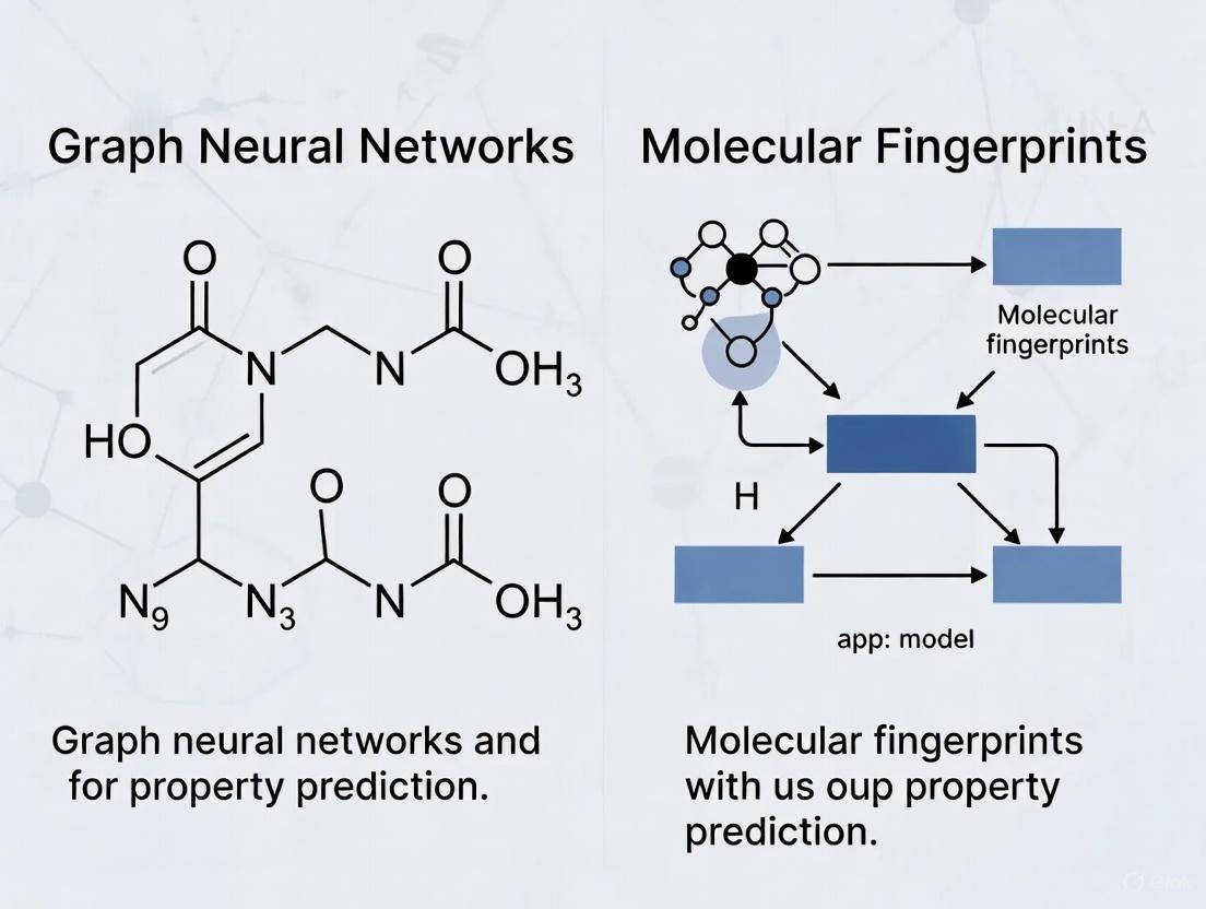
Graph Neural Networks vs. Molecular Fingerprints: A 2025 Benchmark for Molecular Property Prediction
Molecular property prediction is a cornerstone of modern drug discovery and materials science.
Graph Neural Networks vs. Molecular Fingerprints: A 2025 Benchmark for Molecular Property Prediction
Abstract
Molecular property prediction is a cornerstone of modern drug discovery and materials science. This article provides a comprehensive analysis and benchmark of two dominant approaches: traditional molecular fingerprints and advanced graph neural networks (GNNs). Drawing on the latest research, we explore the foundational principles of both methods, detail cutting-edge hybrid architectures like FP-GNN and KA-GNN, and address critical practical considerations such as data requirements, uncertainty estimation, and model interpretability. Through a rigorous comparative validation across diverse property endpoints—from ADMET and toxicity to taste and odor perception—we synthesize evidence-based guidelines for researchers and development professionals to select and optimize the right model for their specific predictive task. The findings reveal a nuanced landscape where the 'best' model is highly context-dependent, and hybrid strategies often provide the most robust solution.
Understanding the Core Technologies: From Handcrafted Fingerprints to Learned Graph Representations
In the field of cheminformatics and drug discovery, molecular fingerprints are a fundamental tool for converting the complex structure of a molecule into a fixed-length, machine-readable bit vector. They enable rapid similarity searching, virtual screening, and the prediction of molecular properties by capturing key structural features. Among the numerous available fingerprints, the Extended-Connectivity Fingerprint (ECFP), the Morgan fingerprint (a common implementation of ECFP), and the PubChem fingerprint have emerged as industry standards. This guide provides a detailed, objective comparison of these fingerprints, frames their performance against modern Graph Neural Networks (GNNs), and outlines the experimental protocols used for their evaluation.
Fingerprint Definitions and Algorithms
The following table summarizes the core characteristics and generation algorithms of the three industry-standard fingerprints.
Table 1: Definition and Key Characteristics of Standard Molecular Fingerprints
| Fingerprint | Type | Core Algorithm | Key Features | Common Uses |
|---|---|---|---|---|
| ECFP / Morgan [1] | Circular (Topological) | Morgan algorithm; iteratively captures circular atom neighborhoods, hashes them into a bit vector [1]. | Captures molecular topology independent of atom numbering; excellent for identifying structurally similar molecules. | Structure-activity modeling, virtual screening, molecular similarity. |
| PubChem Fingerprint [2] | Substructure-based | Encodes the presence or absence of 881 predefined chemical substructures derived from the PubChem database [2]. | Provides a direct, interpretable mapping between bits and specific functional groups or substructures. | Bioactivity prediction, high-throughput screening. |
The generation of these fingerprints, particularly the circular ECFP/Morgan, follows a systematic workflow. The diagram below illustrates the key steps involved in creating an ECFP/Morgan fingerprint.
Fingerprints vs. Graph Neural Networks: A Performance Benchmark
A critical question in modern cheminformatics is whether complex deep learning models like GNNs outperform traditional fingerprint-based methods. Evidence from comprehensive studies reveals a nuanced performance landscape.
Table 2: Comparative Performance of Fingerprint-Based Models vs. Graph Neural Networks
| Model Category | Representative Examples | Key Findings from Experimental Benchmarks | Relative Advantages |
|---|---|---|---|
| Fingerprint-Based Models | SVM, Random Forest (RF), XGBoost using ECFP and other fingerprints [3]. | On average, descriptor-based models (using fingerprints) outperformed graph-based models on 11 public datasets in terms of prediction accuracy and computational efficiency [3]. SVM performed best on regression tasks, while RF and XGBoost were top classifiers [3]. | Computational efficiency, interpretability, and state-of-the-art performance on many ADMET prediction tasks [4]. |
| Graph Neural Networks (GNNs) | GCN, GAT, MPNN, Attentive FP [3]. | Some GNNs (e.g., Attentive FP, GCN) achieved outstanding performance on specific, larger or multi-task datasets [3]. Newer architectures like KA-GNNs show consistent improvements over conventional GNNs [5]. | Potential to automatically learn task-specific features; strong performance on unstructured data like 3D molecular shape [4]. |
| Hybrid Models | FH-GNN (Fingerprint-enhanced GNN) [6]. | Models that integrate hierarchical graph structures with fingerprint features outperformed baseline models, demonstrating the complementary strengths of both approaches [6]. | Combines learned representations from GNNs with expert knowledge from fingerprints. |
The typical methodology for a comparative study, as outlined in the search results, involves a direct, standardized evaluation across multiple datasets and model types, as shown in the workflow below.
Essential Research Reagents and Tools
To implement the experimental protocols cited in this guide, researchers require the following key software tools and databases.
Table 3: Key Research Reagents and Computational Tools
| Item Name | Function / Purpose | Relevant Context / Use Case |
|---|---|---|
| RDKit | An open-source cheminformatics toolkit. | Used for generating Morgan/ECFP fingerprints, reading SMILES strings, and calculating molecular descriptors [3] [7]. |
| MoleculeNet / TDC | Curated benchmarks for molecular machine learning. | Provides standardized datasets (e.g., ESOL, FreeSolv, BBBP) for fair model comparison [3] [4]. |
| DeepPurpose | A molecular modeling and prediction toolkit. | Facilitates the implementation and comparison of various molecular representation methods, including multiple fingerprints and GNNs [2]. |
| CHEMBL / PubChem | Large-scale databases of bioactive molecules. | Sources for experimental bioactivity data used for training and validating predictive models [2] [8]. |
The ECFP/Morgan and PubChem fingerprints remain powerful, efficient, and often superior choices for many molecular property prediction tasks, especially when combined with traditional machine learning models like XGBoost. The choice between fingerprints and GNNs is not a simple dichotomy. Fingerprints excel in computational efficiency and performance on structured data and well-defined tasks, while GNNs show promise in handling unstructured data and for large, multi-task datasets. The most powerful emerging trend is hybrid modeling, which integrates the interpretability and robust performance of fingerprints with the automatic feature-learning capacity of GNNs, offering a synergistic path forward for computational drug discovery [6].
The accurate prediction of molecular properties is a cornerstone of modern drug discovery and materials science, where computational models are essential for reducing the costs and risks of experimental trials. For years, the dominant paradigm relied on molecular fingerprints—expert-crafted vectors encoding specific structural patterns—combined with traditional machine learning models like Random Forest or XGBoost [3] [4]. However, the emergence of Graph Neural Networks (GNNs) has introduced a powerful alternative: end-to-end deep learning models that learn task-specific representations directly from the molecular graph structure itself [3] [9].
This paradigm shift raises a critical question for researchers and development professionals: which approach delivers superior performance for specific property prediction tasks? The answer is not absolute but depends on dataset characteristics, property types, and resource constraints. While GNNs automatically learn hierarchical features from atomic interactions, fingerprints offer computational efficiency and strong baselines, especially on smaller datasets [3] [4]. This guide provides an objective comparison of these competing methodologies, supported by recent experimental data and detailed protocols to inform your research decisions.
How GNNs Learn from Molecular Structures
Fundamental Architecture of Graph Neural Networks
GNNs are specifically designed to process data represented as graphs, making them naturally suited for molecules where atoms constitute nodes and bonds form edges. The core operation of a GNN is the message-passing mechanism, where each atom's representation is iteratively updated by aggregating information from its neighboring atoms [3]. This process enables GNNs to capture the complex topological environment of each atom within the molecular structure.
Advanced GNN Architectures for Molecular Property Prediction
Recent research has produced specialized GNN architectures that extend beyond basic message-passing:
- Fingerprint-Enhanced Hierarchical GNNs (FH-GNN): These models integrate traditional fingerprint features with hierarchical graph learning through adaptive attention mechanisms, simultaneously learning from atomic-level, motif-level, and graph-level information [6].
- Kolmogorov-Arnold GNNs (KA-GNN): This framework replaces standard multilayer perceptrons in GNNs with Kolmogorov-Arnold networks using Fourier-series-based functions, enhancing expressivity and parameter efficiency while improving interpretability by highlighting chemically meaningful substructures [5].
- Equivariant GNNs (EGNN): These models incorporate 3D molecular coordinates while preserving Euclidean symmetries (translation, rotation, reflection), showing particular strength for geometry-sensitive properties like partition coefficients [9].
- Graph Transformers (Graphormer): Applying global attention mechanisms to graph structures, these models excel at capturing long-range dependencies within molecules, achieving state-of-the-art performance on various benchmarks [9].
Experimental Comparison: GNNs vs. Molecular Fingerprints
Benchmarking Protocols and Dataset Specifications
To ensure fair comparisons, researchers typically employ standardized benchmark datasets and evaluation protocols:
Commonly Used Datasets:
- MoleculeNet: A comprehensive collection including QM9 (quantum properties), ESOL (solubility), FreeSolv (solvation energy), Lipop (lipophilicity), and Tox21 (toxicity) [6] [9] [3].
- OGB-MolHIV: A realistic bioactivity classification dataset from the Open Graph Benchmark [9].
- ToxCast: Toxicity prediction dataset with 19-617 tasks, used for assessing real-world scenario performance [10] [3].
Standard Evaluation Metrics:
- Regression Tasks: Mean Absolute Error (MAE), Root Mean Squared Error (RMSE)
- Classification Tasks: Area Under ROC Curve (AUROC), Area Under Precision-Recall Curve (AUPRC), Accuracy, Precision, Recall [11] [9]
Experimental protocols typically involve stratified k-fold cross-validation (commonly k=5) with maintained train/test splits to ensure reliable generalization estimates. For GNN training, standard practice includes early stopping based on validation performance and multiple random initializations to account for variability [11] [3].
Quantitative Performance Comparison
Table 1: Performance Comparison Across Various Molecular Property Prediction Tasks
| Model Category | Specific Model | Dataset | Property Type | Performance Metrics |
|---|---|---|---|---|
| Fingerprint-Based | Morgan FP + XGBoost | Odor Prediction | Multi-label Classification | AUROC: 0.828, AUPRC: 0.237 [11] |
| Fingerprint-Based | Morgan FP + RF | Odor Prediction | Multi-label Classification | AUROC: 0.784, AUPRC: 0.216 [11] |
| GNN | FH-GNN | Multiple MoleculeNet | Classification/Regression | Outperformed baselines on 8 datasets [6] |
| GNN | KA-GNN | 7 Molecular Benchmarks | Multiple | Superior accuracy & computational efficiency vs conventional GNNs [5] |
| GNN | Graphormer | OGB-MolHIV | Bioactivity Classification | ROC-AUC: 0.807 [9] |
| GNN | EGNN | QM9 (log K_d) | Environmental Partitioning | MAE: 0.22 [9] |
| GNN | GPS + Knowledge Graph | Tox21 (NR-AR) | Toxicity Classification | AUC: 0.956 [12] |
Table 2: Computational Efficiency and Data Requirements
| Model Type | Training Time | Data Efficiency | Interpretability | Best-Suited Applications |
|---|---|---|---|---|
| Fingerprint + Traditional ML | Seconds to minutes (large datasets) [3] | Excellent on small datasets [4] | High (via SHAP, feature importance) [3] | Small datasets, rapid prototyping, structured data [4] |
| Standard GNNs | Hours to days | Requires larger datasets [13] | Moderate (attention weights) | General-purpose property prediction [3] |
| Advanced GNNs (Hierarchical, KA) | Similar to standard GNNs | Improved via pre-training | Enhanced (meaningful substructures) [5] | Complex properties requiring hierarchical understanding [6] [5] |
| 3D-Aware GNNs (EGNN) | Higher due to 3D processing | Requires 3D structural data | Moderate | Geometry-sensitive properties (partition coefficients) [9] |
Analysis of Performance Patterns
The experimental data reveals several key patterns:
Fingerprint advantages: On structured data modalities, traditional fingerprints combined with gradient-boosted trees consistently achieve competitive results, with Morgan-fingerprint-based XGBoost delivering AUROC of 0.828 in odor prediction tasks [11]. The Therapeutic Data Commons (TDC) ADMET benchmark shows that approximately 75% of state-of-the-art results are achieved using "old-school" gradient-boosted trees with molecular fingerprints [4].
GNN strengths: GNNs excel in capturing complex spatial relationships and hierarchical structures, with specialized architectures demonstrating particular advantages:
- FH-GNN outperforms baselines by integrating hierarchical molecular graphs with fingerprint features through adaptive attention [6].
- KA-GNN consistently surpasses conventional GNNs in both prediction accuracy and computational efficiency across seven molecular benchmarks [5].
- Knowledge-Enhanced GNNs integrating biological mechanism information (e.g., compound-gene-pathway associations) achieve exceptional performance on toxicity prediction, with GPS model reaching AUC of 0.956 on Tox21 NR-AR task [12].
Data size dependency: GNNs tend to underperform on small datasets, with one comprehensive study finding that descriptor-based models generally outperformed graph-based models across 11 public datasets [3]. Consistency-regularized approaches (CRGNN) have been developed specifically to address this limitation by better utilizing molecular graph augmentation during training [13].
Methodology Deep Dive: Experimental Protocols
Molecular Fingerprint Implementation Protocol
Feature Extraction Process:
- Input Representation: Molecules are represented as SMILES strings or MolBlock representations [11].
- Fingerprint Generation:
- Morgan Fingerprints: Computed using the Morgan algorithm from optimized molecular structures, typically with radius 2 (equivalent to ECFP4) [11].
- Functional Group Fingerprints: Generated by detecting predefined substructures using SMARTS patterns [11].
- Molecular Descriptors: Calculated using RDKit, including molecular weight, hydrogen bond donors/acceptors, topological polar surface area (TPSA), logP, rotatable bonds, heavy atom count, and ring count [11].
- Model Training: Fingerprints are used as input features for traditional machine learning models:
Advantages: This approach benefits from computational efficiency, with XGBoost and Random Forest requiring only seconds to train models even on large datasets [3].
Graph Neural Network Implementation Protocol
Standard GNN Training Workflow:
- Graph Construction: Atoms represented as nodes (with features: atom type, hybridization, valence), bonds as edges (with features: bond type, conjugation) [3].
- Message Passing: Multiple layers (typically 3-6) of neighborhood aggregation using frameworks like:
- Readout Phase: Atom representations are aggregated into molecular-level representations using summation, averaging, or attention-based pooling [3].
- Property Prediction: The molecular representation is passed through fully connected layers for final property prediction [6].
Advanced GNN Training Strategies:
- Consistency Regularization (CRGNN): Applied for small datasets by creating strongly and weakly-augmented views of molecular graphs and encouraging consistent predictions between them [13].
- Knowledge Integration: Incorporating external biological knowledge through heterogeneous graph structures that connect compounds to genes and pathways [12].
- Self-Supervised Pre-training: Leveraging large unlabeled molecular datasets to learn generalizable representations before fine-tuning on specific property prediction tasks [14].
The Scientist's Toolkit: Essential Research Reagents
Table 3: Essential Computational Tools for Molecular Property Prediction
| Tool Name | Type | Primary Function | Application Context |
|---|---|---|---|
| RDKit | Cheminformatics Library | Molecular descriptor calculation, fingerprint generation, SMILES processing [11] | Fundamental preprocessing for both fingerprint and GNN approaches |
| OGG/MoleculeNet | Benchmark Datasets | Standardized molecular property datasets for fair model comparison [9] | Model evaluation and benchmarking across diverse property types |
| PyTor Geometric | Deep Learning Library | GNN implementation and training with molecular graph support [9] | Developing and training custom GNN architectures |
| XGBoost/LightGBM | Traditional ML Library | Gradient boosting implementations for fingerprint-based modeling [11] [3] | Building high-performance fingerprint-based predictors |
| Chemprop | Specialized GNN Framework | Message-passing neural networks specifically designed for molecular property prediction [10] | Rapid implementation of state-of-the-art GNN models |
| TDC (Therapeutic Data Commons) | Benchmark Platform | ADMET-specific benchmarks and datasets [4] | Real-world drug development property prediction |
| Neo4j | Graph Database | Storage and querying of knowledge graphs for biological information [12] | Integrating heterogeneous knowledge into GNN models |
Based on the comprehensive experimental evidence:
Choose Molecular Fingerprints with Traditional ML when:
Choose Graph Neural Networks when:
- Larger datasets are available (> 10,000 compounds) for sufficient training [13] [3]
- Predicting complex properties requiring 3D spatial understanding or hierarchical reasoning [6] [9]
- Integrating heterogeneous biological knowledge is beneficial for the task [12]
- Capturing long-range dependencies or complex molecular interactions is essential [5] [9]
Consider Hybrid Approaches when:
- Seeking to balance predictive performance with uncertainty estimation (neural fingerprints with Random Forest) [10]
- Addressing data scarcity issues while leveraging GNN strengths (consistency-regularized GNNs) [13]
- Combining structural information with external knowledge for mechanistically informed predictions [14] [12]
The most advanced applications are increasingly leveraging integrated approaches, such as fingerprint-enhanced hierarchical GNNs or knowledge graph-augmented networks, which combine the complementary strengths of both paradigms [6] [12]. As the field evolves, the optimal solution typically involves selecting architectures based on specific dataset characteristics, property complexity, and available computational resources rather than adhering to a one-size-fits-all approach.
In the field of molecular property prediction, a central debate exists between traditional descriptor-based methods using molecular fingerprints and modern graph neural networks. Molecular fingerprints, such as Extended Connectivity Fingerprints (ECFPs), employ predefined structural keys and hashing algorithms to represent molecules as fixed-length vectors [15] [3]. In contrast, GNNs learn representations directly from the molecular graph structure, where atoms constitute nodes and bonds form edges [16]. While early studies suggested GNNs might universally outperform fingerprint-based approaches, more comprehensive benchmarks reveal a nuanced reality where model performance depends significantly on dataset characteristics, task requirements, and architectural selection [3].
This guide provides an objective comparison of three fundamental GNN architectures—MPNN, GAT, and GCN—within this broader context, presenting experimental data to inform researchers' model selection for drug discovery applications.
Core Architectural Principles and Mechanisms
Table 1: Core Computational Mechanisms of GNN Architectures
| Architecture | Core Operational Principle | Mathematical Formulation | Key Hyperparameters |
|---|---|---|---|
| GCN | Spectral-based convolution with symmetric normalization [17] | ( H^{(l+1)} = \sigma(\tilde{D}^{-\frac{1}{2}}\tilde{A}\tilde{D}^{-\frac{1}{2}} H^{(l)}W^{(l)}) ) | Number of graph convolution layers, Units per layer (e.g., [64,64], [128,128]) [16] |
| GAT | Attention-weighted neighborhood aggregation [16] [17] | ( \alpha{ij} = \text{softmax}(\text{LeakyReLU}(\vec{a}^T[Whi|Wh_j])) ) | Attention heads, Dropout rate [16] |
| MPNN | Message functions with permutation-invariant aggregation [17] | ( m{ij} = fe(hi,hj,e{ij});\ hi' = fh(hi, \sum{j \in Ni} m_{ij}) ) | Number of atom output features, Message passing steps [16] |
Figure 1: Computational workflows of GCN, GAT, and MPNN architectures illustrating their distinct approaches to graph-based feature learning.
Key Differentiating Architectural Features
GCN employs spectral graph convolutions with symmetric normalization of the graph Laplacian, enabling localized first-order neighborhood aggregation. The renormalization trick (( I + D^{-1/2}AD^{-1/2} \rightarrow \tilde{D}^{-1/2}\tilde{A}\tilde{D}^{-1/2} )) addresses gradient instability issues in deeper architectures [17].
GAT introduces attention mechanisms that compute adaptive weights for neighborhood aggregation, allowing the model to prioritize more influential neighboring nodes. Multi-head attention extends this capability to capture different aspects of structural relationships [16] [17].
MPNN provides a generalized framework for message passing where each node receives messages from its neighbors, aggregates them, and updates its state accordingly. This approach explicitly separates message construction, aggregation, and node update functions, offering greater flexibility in modeling complex molecular interactions [17].
Experimental Performance Comparison
Quantitative Benchmarking Across Molecular Prediction Tasks
Table 2: Performance Comparison of GNN Architectures on Molecular Property Prediction Tasks
| Task Domain | Best Performing Architecture | Key Metric | Comparative Performance | Reference Dataset |
|---|---|---|---|---|
| Cross-Coupling Reaction Yield Prediction | MPNN | R² = 0.75 | Outperformed GCN, GAT, GraphSAGE, GIN [18] | Diverse transition metal-catalyzed cross-coupling reactions [18] |
| Acute Toxicity Prediction | Attentive FP (GAT variant) | Lowest MSE | 12.3-13.3% improvement over second-best GCN [16] | Fish, Daphnia magna, Tetrahymena pyriformis [16] |
| Activity Cliff Sensitivity | ECFP Fingerprints | Slope >1 in dissimilarity analysis | GCN, GAT, MPNN all showed lower sensitivity to subtle structural changes [15] | MoleculeACE benchmark [15] |
| General Molecular Property Prediction | Descriptor-based models (SVM, XGBoost) | Prediction accuracy | Outperformed GCN, GAT, MPNN on average across 11 datasets [3] | MoleculeNet benchmarks [3] |
Task-Specific Performance Patterns
Reaction Yield Prediction: In heterogeneous datasets encompassing Suzuki, Sonogashira, and other cross-coupling reactions, MPNN demonstrated superior predictive capability (R²=0.75), potentially due to its flexible message functions effectively capturing complex reaction pathways [18].
Toxicity Prediction: For acute toxicity tasks across four different species, Attentive FP (a GAT variant) achieved the lowest prediction error, with attention mechanisms providing interpretable atomic heatmaps highlighting chemically significant substructures [16].
Handling Subtle Structural Changes: Traditional ECFPs demonstrated greater sensitivity to minor structural modifications that cause significant potency differences (activity cliffs), with graph embeddings from GCN, GAT, and MPNN showing compressed representational distances between structurally similar molecules [15].
Experimental Protocols and Methodologies
Standardized Evaluation Frameworks
Dataset Splitting: Common practice employs random splits with 80% for training and 20% for testing, with five-fold cross-validation applied on the training set, effectively creating 64%/16%/20% divisions for training/validation/testing respectively [16].
Hyperparameter Tuning: Critical parameters include batch size (typically 32-128), dropout rate (0-0.2), number of GNN layers (1-4), and hidden layer dimensions (64-256 units). Systematic exploration of full parameter combinations is recommended for optimal performance [16].
Performance Metrics: Standard evaluation employs Mean Squared Error (MSE), Mean Absolute Percentage Error (MAPE), and R² values for regression tasks, with attention to both predictive accuracy and model interpretability [18] [16].
Emerging Hybrid and Enhanced Architectures
Recent architectural innovations address limitations of standard GNNs:
KA-GNNs: Kolmogorov-Arnold GNNs integrate Fourier-based KAN modules into node embedding, message passing, and readout components, demonstrating enhanced accuracy and computational efficiency on molecular benchmarks [5].
FH-GNN: Fingerprint-enhanced hierarchical GNNs combine atomic-level, motif-level, and graph-level information with chemical fingerprints using adaptive attention mechanisms, outperforming baseline models on multiple MoleculeNet datasets [6].
GraphCliff: Specifically designed to address activity cliff challenges through short-long range gating mechanisms, improving discrimination of structurally similar molecules with different properties [15].
Table 3: Essential Computational Tools for GNN Molecular Property Prediction Research
| Tool Category | Specific Implementation | Research Function | Application Context |
|---|---|---|---|
| Graph Representation | RDKit [3] | Molecular graph construction from SMILES | Preprocessing pipeline for all GNN architectures |
| Fingerprint Generation | ECFP [15] [3] | Baseline molecular representation | Comparative performance benchmarking |
| Core GNN Frameworks | MPNN, GCN, GAT [16] | Fundamental architectural implementations | Baseline model development and ablation studies |
| Advanced Architectures | Attentive FP [16], KA-GNN [5] | Specialized property prediction | High-accuracy molecular modeling |
| Interpretability Tools | Integrated Gradients [18], SHAP [3] | Model decision explanation | Mechanistic insight and validation |
| Benchmark Datasets | MoleculeNet [3], MoleculeACE [15] | Standardized performance evaluation | Comparative architecture assessment |
The comparative analysis reveals that no single GNN architecture universally dominates molecular property prediction. MPNNs demonstrate particular strength for reaction yield prediction, likely due to their flexible message-passing mechanisms capturing complex transformation pathways [18]. GAT-based models like Attentive FP excel in toxicity prediction tasks where attention mechanisms provide both performance and interpretability benefits [16]. GCNs offer solid baseline performance with computational efficiency but may lack sensitivity to subtle structural changes critical for activity cliff identification [15].
For researchers navigating the GNN versus molecular fingerprints decision, the experimental evidence suggests that traditional fingerprint-based methods remain competitive, particularly for smaller datasets or when subtle structural changes significantly impact properties [3]. However, GNNs offer advantages in end-to-end learning without manual feature engineering and increasingly outperform fingerprints as dataset size and structural complexity increase, especially with emerging hybrid architectures that integrate fingerprint-enhanced approaches [6] and novel mechanisms like Fourier-based KAN modules [5].
Strategic architecture selection should consider dataset size, structural complexity, requirement for interpretability, and computational resources, with the understanding that the field continues to evolve through architectures specifically designed to address current limitations in molecular representation learning.
The accurate prediction of molecular properties is a critical task in computational drug discovery and materials science, driving the need for robust and efficient machine learning models. The central challenge lies in selecting the optimal molecular representation, which dictates how the raw structural information of a compound is encoded for a machine learning algorithm. This guide provides an objective comparison between two dominant paradigms: molecular fingerprints, which are fixed, hand-crafted vectors representing predefined substructures, and graph neural networks (GNNs), which learn representations directly from the atomic graph structure of a molecule. The choice between these input modalities involves fundamental trade-offs between representational capacity, data efficiency, computational demand, and interpretability, which this article explores through recent experimental evidence and detailed methodological breakdowns.
Core Concepts and Methodologies
Molecular Fingerprints: Structured Vector Representations
Molecular fingerprints are fixed-length vector representations where specific bits or components correspond to the presence or absence of predefined molecular substructures or features [19].
- Extended-Connectivity Fingerprints (ECFP): Among the most common, ECFPs are circular fingerprints that capture atom environments within a specified radius. They are generated using a hashing procedure to map each identified substructure to a set of bits in the fixed-length vector [19] [11].
- Generation Workflow: The typical generation process begins with a molecule's SMILES string. The Morgan algorithm, often implemented via toolkits like RDKit, is then used to enumerate all circular substructures around each atom up to a given radius. These substructures are then hashed into a bit vector of fixed length [11].
- Model Integration: The resulting fingerprint vector serves as a high-dimensional input feature for classical machine learning models. Common algorithms include Random Forest (RF), Support Vector Machines (SVM), and gradient-boosting frameworks like XGBoost and LightGBM [11] [10].
Graph Neural Networks: Learned Graph Representations
Graph Neural Networks (GNNs) are a class of deep learning models designed to operate directly on graph-structured data. A molecule is naturally represented as a graph, where atoms are nodes and bonds are edges [20].
- Model Architecture: A typical GNN for molecules consists of several key layers [21]:
- Node Embedding: Initializes each atom node with a feature vector (e.g., atom type, charge).
- Message Passing: In multiple stacked layers, each node aggregates feature information from its neighboring nodes. This step allows the model to capture the local chemical environment of each atom [20].
- Graph Pooling (Readout): After several message-passing layers, the node representations are aggregated into a single, fixed-dimensional vector that represents the entire molecule. This vector is then passed to a standard neural network to make a property prediction [21].
- Permutation Invariance: A key property of GNNs is that they are designed to be invariant to the ordering of atoms and bonds, ensuring the same molecule always produces the same representation regardless of how its graph is presented [20].
Performance Benchmarking and Comparative Analysis
Predictive Performance on Standard Tasks
Recent comparative studies provide quantitative benchmarks for fingerprint-based and GNN-based models across various molecular property prediction tasks.
Table 1: Performance Comparison on Odor Prediction (Multi-label Classification)
| Model Combination | Feature Set | AUROC | AUPRC | Accuracy (%) | Precision (%) | Recall (%) |
|---|---|---|---|---|---|---|
| XGBoost | Morgan Fingerprints (ST) | 0.828 | 0.237 | 97.8 | 41.9 | 16.3 |
| XGBoost | Molecular Descriptors (MD) | 0.802 | 0.200 | - | - | - |
| XGBoost | Functional Groups (FG) | 0.753 | 0.088 | - | - | - |
| Random Forest | Morgan Fingerprints (ST) | 0.784 | 0.216 | - | - | - |
| LightGBM | Morgan Fingerprints (ST) | 0.810 | 0.228 | - | - | - |
Source: Adapted from a comparative study on odor decoding using a dataset of 8,681 compounds [11].
The data in Table 1 demonstrates that a classical machine learning model (XGBoost) paired with Morgan fingerprints achieved the highest discrimination performance on this complex sensory prediction task, surpassing descriptor-based models and other tree-based algorithms [11].
Table 2: Performance and Uncertainty on ToxCast Tasks
| Model | Average Balanced Accuracy | Uncertainty Estimation Quality |
|---|---|---|
| Chemprop (GNN) | ~0.6 - 0.8 | Moderate |
| Random Forest + Neural Fingerprints | Slightly lower than Chemprop | High and robust |
| SVM + Neural Fingerprints | Comparable to RF+FP | High |
Source: Summarized from an analysis of uncertainty on 19 ToxCast datasets [10].
Table 2 highlights a different trade-off. While a native GNN model (Chemprop) may have a slight edge in pure predictive performance on some toxicity tasks, fingerprint-based models combined with classical ML methods can provide significantly better and more robust uncertainty estimates, a critical feature for real-world industrial decision-making [10].
Advanced GNN Architectures and Hybrid Approaches
Researchers have developed advanced GNN frameworks to overcome limitations of basic models. For instance, Stable-GNN (S-GNN) was proposed to address the performance degradation of GNNs under Out-of-Distribution (OOD) data, a common scenario in real-world applications. By using a feature sample weighting decorrelation technique, S-GNN aims to extract genuine causal features and eliminate spurious correlations, thereby improving generalization and stability on unseen data distributions [21].
Another powerful approach is the integration of GNNs with external biological knowledge. One study constructed a Toxicological Knowledge Graph (ToxKG) incorporating entities like genes and pathways. Heterogeneous GNN models (e.g., GPS, HGT) that leveraged this structured biological knowledge significantly outperformed traditional models using only structural fingerprints on the Tox21 dataset, achieving an AUC of up to 0.956 for specific toxicity endpoints [12].
Experimental Protocols and Workflows
Protocol A: Fingerprint-Based Model Training
The following is a standard workflow for building a molecular property predictor using fingerprints [19] [11].
- Data Curation: Assemble a dataset of molecules, typically represented by SMILES strings, alongside their experimentally measured properties.
- Fingerprint Generation: Use a cheminformatics toolkit like RDKit to compute fingerprints (e.g., ECFP4, Morgan) for every molecule in the dataset. This results in a feature matrix (X) and a target vector (y).
- Model Training: Split the data into training and test sets. Train a classical machine learning model, such as Random Forest or XGBoost, on the training fingerprint vectors.
- Evaluation: Use the held-out test set to evaluate the model's performance using metrics like AUC, accuracy, or mean squared error, depending on the task.
Diagram 1: Fingerprint-based model workflow.
Protocol B: Graph Neural Network Training
The workflow for a GNN-based predictor involves an end-to-end learning process [20] [21].
- Graph Construction: Convert each molecule's SMILES string into a graph object where nodes (atoms) are labeled with features (e.g., element, degree) and edges (bonds) are labeled with their type (e.g., single, double).
- Model Definition: Instantiate a GNN architecture. This typically includes:
- An encoder to create initial node embeddings.
- Multiple message-passing layers to refine node features.
- A global pooling (readout) layer to create a graph-level representation.
- A final feed-forward network for the prediction.
- End-to-End Training: The model is trained via backpropagation. The loss is computed by comparing the model's predictions against the true properties, and the weights across the entire network are updated simultaneously.
Diagram 2: GNN-based model workflow.
The Scientist's Toolkit: Essential Research Reagents
Table 3: Key Software and Data Resources for Molecular Property Prediction
| Resource Name | Type | Primary Function | Relevance |
|---|---|---|---|
| RDKit | Cheminformatics Library | Generation of molecular fingerprints (ECFP, Morgan), descriptors, and graph structures from SMILES. | Foundational for both fingerprint and GNN data preprocessing [19] [11]. |
| PyTorch / TensorFlow | Deep Learning Framework | Provides building blocks and auto-differentiation for constructing and training custom GNN architectures. | Essential for implementing and training GNN models [22]. |
| TUDatasets / OGB | Graph Dataset Repositories | Curated benchmarks for graph machine learning, including molecular datasets like Tox21 and QM9. | Standardized datasets for training and fair model evaluation [21]. |
| PubChem | Chemical Database | Source of SMILES strings, compound identifiers (CIDs), and associated biological assay data. | Primary source for curating custom datasets and gathering molecular structures [12]. |
| Neo4j | Graph Database | Storage and querying of large-scale knowledge graphs (e.g., ToxKG) that integrate chemical and biological data. | Enables advanced GNN models that incorporate external biological context [12]. |
The choice between molecular fingerprints and graph neural networks is not a matter of declaring one universally superior. The optimal input modality is dictated by the specific research context. Molecular fingerprints paired with classical ML models offer a robust, computationally efficient, and often highly competitive baseline, especially on tasks where well-defined substructures are strong predictors and where reliable uncertainty quantification is paramount [11] [10]. In contrast, GNNs excel at end-to-end representation learning from raw structural data, can capture complex topological patterns beyond predefined substructures, and provide a flexible framework for integrating multimodal data, as evidenced by knowledge-graph-enhanced models [12]. For applications demanding maximum predictive performance and where large, high-quality datasets are available, GNNs present a powerful solution. However, for many practical scenarios, particularly those with limited data or a need for high interpretability and robust uncertainty, fingerprint-based models remain a formidable and pragmatic choice. A promising future direction lies in hybrid approaches that leverage the structured prior knowledge of fingerprints within the flexible, learning-based framework of GNNs.
Implementation and Advanced Architectures: From Standalone Models to Hybrid Frameworks
In the field of computational chemistry and drug discovery, the accurate prediction of molecular properties from chemical structure is a fundamental task that directly impacts the efficiency of identifying promising therapeutic candidates. Historically, this challenge has been approached through two primary paradigms: descriptor-based methods that rely on expert-crafted molecular features and fingerprints, and graph-based methods that utilize end-to-end deep learning models such as graph neural networks (GNNs) to automatically learn representations from molecular graphs. While GNNs have garnered significant attention in recent literature, extensive benchmarking studies reveal that traditional fingerprint-based approaches, particularly when combined with powerful tree-based algorithms like XGBoost and Random Forest (RF), remain highly competitive and often superior in terms of predictive accuracy, computational efficiency, and interpretability [3].
The core premise of this guide aligns with emerging evidence that questions the automatic superiority of GNNs. A comprehensive 2021 comparison study concluded that "on average the descriptor-based models outperform the graph-based models in terms of prediction accuracy and computational efficiency" [3]. Similarly, a 2025 study on odor perception modeling found that a Morgan-fingerprint-based XGBoost model achieved the highest discrimination (AUROC 0.828), consistently outperforming descriptor-based models [11]. This guide provides a detailed methodological framework for implementing high-performance fingerprint-based pipelines, objectively compares their performance against contemporary GNN alternatives, and contextualizes these findings within the broader landscape of molecular property prediction research.
Experimental Benchmarking: Fingerprint-Based Models vs. Graph Neural Networks
Quantitative Performance Comparison
Recent comparative studies across diverse molecular property prediction tasks provide compelling evidence for the continued competitiveness of fingerprint-based approaches paired with tree-based models. The following table synthesizes key performance metrics from multiple benchmark studies:
Table 1: Performance comparison of fingerprint-based models versus GNNs across various benchmark datasets
| Dataset/Task | Best Fingerprint-Based Model | Performance | Best GNN Model | Performance | Performance Advantage |
|---|---|---|---|---|---|
| Odor Perception [11] | Morgan Fingerprint + XGBoost | AUROC: 0.828, AUPRC: 0.237 | - | - | Fingerprint + XGBoost |
| BBB Permeability [23] | MACCS Fingerprint + DNN | Accuracy: 97.8%, ROC-AUC: 0.98 | - | - | Fingerprint + DNN |
| Molecular Property Prediction (11 datasets) [3] | Descriptors+Fingerprints + SVM/XGBoost/RF | Best overall average across regression and classification | Attentive FP, GCN | Variable performance across datasets | Fingerprint-Based Models |
| ToxCast (19 datasets) [10] | Neural Fingerprint + Random Forest/SVC | Competitive performance with improved uncertainty | Native Chemprop GNN | Slightly higher prediction performance | Context-Dependent |
The superiority of fingerprint-based approaches is particularly evident in specific domains such as odor prediction, where Morgan-fingerprint-based XGBoost achieved the highest discrimination metrics in a 2025 benchmark study [11]. Similarly, for blood-brain barrier (BBB) permeability prediction, a fingerprint-based deep neural network model achieved remarkable accuracy of 97.8% [23]. Even in direct comparisons with specialized GNN architectures like Attentive FP and GCN, traditional descriptor-based models frequently matched or exceeded graph-based performance across multiple benchmark datasets [3].
Computational Efficiency Assessment
Beyond raw predictive accuracy, computational requirements present another critical dimension for model evaluation, particularly in large-scale virtual screening scenarios:
Table 2: Computational efficiency comparison between fingerprint-based and GNN approaches
| Model Type | Training Time | Inference Speed | Resource Requirements | Implementation Complexity |
|---|---|---|---|---|
| Fingerprint + XGBoost/RF | Seconds to minutes for large datasets [3] | Very fast | Moderate CPU/Memory | Low (established libraries) |
| Graph Neural Networks (GCN, GAT, MPNN) | Hours to days [3] | Slower due to graph processing | High (GPU acceleration beneficial) | High (specialized expertise) |
| Hybrid Models (GNN + Fingerprints) | Moderate to high [6] [24] | Moderate | High (GPU typically required) | Very High |
As evidenced by multiple studies, tree-based models like XGBoost and Random Forest demonstrate exceptional computational efficiency, requiring "only a few seconds to train a model even for a large dataset" [3]. This efficiency advantage extends beyond training to inference phases, making fingerprint-based approaches particularly suitable for high-throughput virtual screening applications where computational resources or time may be constrained.
Uncertainty Estimation and Interpretability
The reliability of predictive models depends not only on accuracy but also on calibrated uncertainty estimates and interpretability. A 2025 study examining uncertainty estimation found that "neural fingerprints combined with classical machine learning methods exhibit a slight decrease in prediction performance compared to the native Chemprop model," but importantly, "provide significantly improved uncertainty estimates" [10]. This characteristic is particularly valuable in real-world industrial applications where understanding prediction confidence directly impacts decision-making.
For interpretability, fingerprint-based models benefit from well-established feature importance methods and model explanation techniques like SHAP (SHapley Additive exPlanations), which can effectively "explore the established domain knowledge for the descriptor-based models" [3]. This interpretability advantage facilitates deeper chemical insights and supports rational molecular design in ways that are often more challenging with complex GNN architectures.
Methodological Framework: Implementing a Fingerprint-Based Pipeline
Experimental Workflow for Fingerprint-Based Modeling
The following diagram illustrates the comprehensive workflow for building a fingerprint-based molecular property prediction pipeline, integrating feature engineering with RDKit and model training with XGBoost/RF:
Molecular Property Prediction Pipeline: From chemical structures to validated predictive models
Detailed Experimental Protocols
Data Curation and Preprocessing
Robust model development begins with rigorous data curation. For molecular property prediction, this involves:
- Data Sourcing: Assemble datasets from multiple expert-curated sources such as ChEMBL, PubChem, or specialized databases relevant to the target property [11] [25]. For odor prediction, researchers unified "ten expert-curated sources" to create a dataset of 8,681 unique odorants [11].
- Standardization: Apply consistent processing to molecular structures using tools like RDKit, including normalization of tautomeric states, removal of duplicates, and standardization of stereochemistry representation [23].
- Descriptor Calculation: Compute comprehensive molecular descriptors using RDKit's built-in functionality, including key physicochemical properties such as molecular weight (MolWt), topological polar surface area (TPSA), octanol-water partition coefficient (molLogP), hydrogen bond donors/acceptors, rotatable bonds count, and ring systems [11] [25].
- Class Imbalance Handling: For classification tasks, employ resampling techniques such as SMOTE, ADASYN, or TOMEK links when facing significant class imbalance, as demonstrated in BBB permeability prediction research [23].
Feature Engineering with RDKit
Effective feature engineering forms the foundation of successful fingerprint-based models:
- Morgan Fingerprints (ECFP-like): Generate circular topological fingerprints using the Morgan algorithm, typically with radius 2 (equivalent to ECFP4) and bit lengths of 1024 or 2048 [11] [25]. These fingerprints effectively capture molecular substructures and have demonstrated superior performance in benchmarking studies [11].
- MACCS Keys: Implement predefined structural keys (166 bits) that encode specific chemical substructures and functional groups, particularly valuable for capturing pharmacophoric features [23].
- Functional Group Fingerprints: Create binary fingerprints indicating the presence or absence of specific functional groups using SMARTS patterns to define relevant chemical substructures [11].
- Descriptor Computation: Calculate comprehensive molecular descriptors using RDKit, including topological, constitutional, and physicochemical properties that provide complementary information to structural fingerprints [3].
Model Training with XGBoost and Random Forest
Optimized training protocols for tree-based models:
- Data Splitting: Implement stratified splitting (typically 80:20 train:test ratio) to maintain class distribution, with optional nested cross-validation for hyperparameter optimization [11] [23].
- Hyperparameter Tuning: For XGBoost, optimize critical parameters including learning rate (η), maximum tree depth, subsampling rates, and L1/L2 regularization strengths [11]. For Random Forest, tune the number of trees, maximum features per split, and maximum depth [25].
- Multi-label Support: Configure models to support multi-label classification where molecules can simultaneously exhibit multiple properties (e.g., "Floral" and "Spicy" odor characteristics) using One-vs-Rest or specialized multi-output strategies [11].
- Evaluation Metrics: Employ comprehensive evaluation metrics including Area Under the Receiver Operating Characteristic (AUROC), Area Under the Precision-Recall Curve (AUPRC), accuracy, precision, recall, and F1-score, with particular emphasis on AUROC and AUPRC for imbalanced datasets [11] [25].
Table 3: Essential tools and resources for implementing fingerprint-based molecular property prediction pipelines
| Tool/Resource | Type | Primary Function | Application Notes |
|---|---|---|---|
| RDKit [11] [25] | Open-source Cheminformatics Library | Molecular descriptor calculation, fingerprint generation, structural standardization | Core dependency for feature engineering; provides multiple fingerprint types and 200+ molecular descriptors |
| XGBoost [11] | Machine Learning Library | Gradient boosting implementation for model training | Excels with high-dimensional fingerprint data; superior performance with Morgan fingerprints |
| Random Forest [25] | Machine Learning Library | Ensemble learning with decision trees | Robust to noise; provides native feature importance estimates |
| Scikit-learn [25] | Machine Learning Library | Data preprocessing, model evaluation, auxiliary algorithms | Essential for data splitting, preprocessing, and performance metrics calculation |
| SHAP [25] | Model Interpretation Library | Explainable AI for model predictions | Identifies influential molecular features and substructures driving predictions |
| PubChem [11] | Chemical Database | Compound information and structure retrieval | Source for canonical SMILES and compound metadata via PUG-REST API |
| PyRfume [11] | Data Repository | Curated olfactory datasets | Example of domain-specific data source for model development |
Comparative Analysis: When to Choose Fingerprint-Based Approaches vs. GNNs
Technical and Practical Considerations
The choice between fingerprint-based pipelines and graph neural networks involves multiple technical and practical considerations:
Table 4: Decision framework for selecting between fingerprint-based and GNN approaches
| Consideration | Fingerprint + XGBoost/RF | Graph Neural Networks |
|---|---|---|
| Data Efficiency | Excellent performance with small to medium datasets (n < 10,000) [3] | Typically requires larger datasets for optimal performance |
| Computational Resources | Suitable for CPU-based environments; minimal hardware requirements [3] | GPU acceleration strongly recommended; substantial memory requirements |
| Interpretability Needs | High (native feature importance + SHAP explanations) [25] [3] | Moderate to Low (requires specialized interpretation techniques) |
| Implementation Timeline | Rapid prototyping and iteration (hours to days) [3] | Extended development cycles (weeks to months) |
| Representation Flexibility | Fixed molecular representation | Adaptive, task-specific representation learning |
| Uncertainty Estimation | Well-calibrated probabilities with Random Forest [10] | Variable calibration; may require specialized techniques |
Emerging Hybrid Approaches
Recent research has explored hybrid architectures that combine the strengths of both paradigms, integrating "hierarchical molecular graphs and fingerprints" to create more powerful predictive models [6]. These approaches simultaneously learn "from hierarchical molecular graphs and fingerprints" using "adaptive attention mechanism to balance the importance of hierarchical graphs and fingerprint features" [6]. Similarly, the Multi-Level Fusion Graph Neural Network (MLFGNN) incorporates "molecular fingerprints as a complementary modality" to enhance model performance [24]. Such hybrid strategies represent a promising direction for future methodology development, potentially mitigating the limitations of both pure fingerprint-based and pure graph-based approaches.
Empirical evidence from recent benchmarking studies consistently demonstrates that fingerprint-based pipelines utilizing RDKit for feature engineering and XGBoost/Random Forest for model training remain highly competitive for molecular property prediction tasks. These approaches offer compelling advantages in terms of predictive performance, computational efficiency, implementation simplicity, and model interpretability. While graph neural networks provide valuable capabilities for automated feature learning and may excel in specific scenarios, fingerprint-based methods establish a strong baseline that should be included in any comprehensive molecular property prediction workflow. The continued development of hybrid approaches that combine molecular fingerprints with graph-based architectures represents a promising research direction that may further advance the state of the art in computational molecular modeling.
The accurate prediction of molecular properties is a cornerstone of modern chemical and pharmaceutical research. The fundamental challenge lies in identifying optimal representations of molecular structure that can be leveraged by machine learning models. Two dominant paradigms have emerged: molecular fingerprints, which are human-engineered vector representations encoding specific chemical substructures and properties, and graph neural networks (GNNs), which learn representations directly from the molecular graph structure where atoms constitute nodes and bonds form edges [2]. This guide provides a practical examination of implementing GNN models, with particular focus on the critical steps of atom and bond featureization and the construction of effective training loops, while contextualizing performance against traditional fingerprint-based approaches.
Molecular Representation Methodologies
Molecular Fingerprints: Traditional Feature Engineering
Molecular fingerprints represent molecules as fixed-length vectors encoding structural information through predefined rules. Several fingerprinting methods are commonly employed, each capturing different aspects of molecular structure [2]:
- Morgan Fingerprints (Circular Fingerprints): Encode structural information by considering substructures at different radii around each atom, providing a conformation-independent representation of molecular topology.
- PubChem Fingerprints: Binary fingerprints derived from the PubChem Compound database, representing molecular structural features based on a large dictionary of predefined chemical substructures.
- RDKit Fingerprints: A fingerprinting method integrated within the RDKit cheminformatics package, generating bit vectors based on molecular substructures with dictionary entries for each set bit.
- ErG Fingerprints: Employ pharmacophore-type node descriptions to encode relevant molecular properties and spatial relationships, capturing different chemical information than path-based fingerprints.
These hand-crafted representations have demonstrated utility in Quantitative Structure-Activity Relationship (QSAR) and Quantitative Structure-Property Relationship (QSPR) studies, but inherently limit the model to pre-specified chemical patterns and may fail to capture novel structural motifs relevant to specific property prediction tasks [2].
Graph Neural Networks: Learned Representations
GNNs operate directly on the molecular graph structure, learning task-specific representations through message passing between connected nodes (atoms). The fundamental operation of a GNN layer involves aggregating information from a node's neighbors and updating the node's feature representation accordingly [26]. A basic Graph Convolutional Network (GCN) layer can be implemented as follows [26]:
Advanced GNN architectures have been developed specifically for molecular property prediction. The Atomistic Line Graph Neural Network (ALIGNN) explicitly models both two-body (bond) and three-body (angle) interactions by performing message passing on both the atomistic bond graph and its line graph corresponding to bond angles [27]. This approach directly incorporates angular information critical for many molecular properties, moving beyond distance-based representations to capture more complex geometric features.
Atom and Bond Featureization Strategies
Atom Featureization
The initial step in GNN implementation involves representing atoms as feature vectors encoding chemically relevant information. The ALIGNN framework utilizes 9 input node features based on atomic species [27]:
- Electronegativity
- Group number
- Covalent radius
- Valence electrons
- First ionization energy
- Electron affinity
- Block (s, p, d, f)
- Atomic volume
These features provide the model with fundamental chemical information about each atom, enabling it to learn relationships between elemental properties and molecular behavior.
Bond and Angle Featureization
Beyond atom features, bond representations are crucial for capturing molecular topology. ALIGNN initializes edge features as interatomic bond distances, expanded using a radial basis function (RBF) expansion with support between 0-8 Å for crystals and up to 5 Å for molecules [27]. For angle information, ALIGNN uses an RBF expansion of bond angle cosines, calculated as θ = arccos((rij · rjk)/(|rij||rjk|)), where rij and rjk are atomic displacement vectors between atoms i, j, and k [27].
The ALIGNN update mechanism alternates between graph convolution on the bond graph and its line graph, enabling the propagation of bond angle information through interatomic bond representations to the atom-wise representations and vice versa [27]. This dual-graph approach allows the model to explicitly leverage angular information that is critical for many molecular properties but challenging to capture in standard GNN architectures.
Experimental Comparison: GNNs vs. Fingerprints
Performance Benchmarking
A comprehensive comparative analysis evaluated various molecular representations on taste prediction tasks using a dataset of 2601 molecules [2]. The results demonstrated the superior performance of GNN-based approaches:
Table 1: Performance comparison of molecular representation methods for taste prediction [2]
| Representation Method | Prediction Accuracy | Key Advantages | Limitations |
|---|---|---|---|
| GNN-based Models | Highest reported accuracy | Learns task-specific features directly from graph structure; captures complex topological patterns | Computationally intensive; requires careful hyperparameter tuning |
| Morgan Fingerprints | Competitive performance | Conformation-independent; well-established interpretation methods | Limited to predefined substructures; may miss novel patterns |
| PubChem Fingerprints | Moderate performance | Large dictionary of chemical substructures | Dependent on PubChem's specific substructure definitions |
| RDKit Fingerprints | Moderate performance | Integrated with popular cheminformatics toolkit | Similar limitations to other predefined fingerprint methods |
| Consensus Models (Fingerprints + GNN) | Improved performance over individual methods | Combines strengths of engineered and learned features | Increased model complexity |
The study found that consensus models combining GNNs with molecular fingerprints demonstrated the best performance, highlighting the complementary strengths of learned and engineered features [2]. This suggests that fingerprint features may capture some chemical information not immediately accessible to GNNs from graph structure alone, possibly due to the predefined chemical knowledge embedded in fingerprint designs.
Advanced GNN Architectures and Their Performance
Recent GNN advancements have further improved molecular property prediction capabilities:
Fingerprint-enhanced Hierarchical GNN (FH-GNN): Integrates hierarchical molecular graphs (atomic-level, motif-level, graph-level) with traditional fingerprint features, using an adaptive attention mechanism to balance their importance. This architecture outperformed baseline models on eight benchmark datasets from MoleculeNet [6].
Quantized GNN Models: Address computational efficiency concerns by integrating GNN models with quantization algorithms like DoReFa-Net, reducing memory footprint and computational demands while maintaining predictive performance. Studies show that 8-bit quantization preserves performance on quantum mechanical property prediction tasks, though aggressive 2-bit quantization significantly degrades performance [28].
ALIGNN for Materials Property: Demonstrates improved performance on 52 solid-state and molecular properties from JARVIS-DFT, Materials Project, and QM9 databases, outperforming previous GNN models while maintaining comparable training speed. The explicit incorporation of angle information provides particular benefits for electronic properties sensitive to geometric distortions [27].
Implementation Guide: Training Loops and Optimization
GNN Training Workflow
The training loop for GNNs follows the standard deep learning paradigm with graph-specific considerations [26]:
Graph Representation: Convert molecular structures to graph representations with node features (atoms), edge indices (bonds), and optional edge attributes.
Mini-batching: Combine multiple graphs into a single batch using techniques like zero-padding or more advanced approaches such as stacking adjacency matrices in a block-diagonal form.
Forward Pass: Perform message passing through multiple GNN layers to update node representations based on neighborhood information.
Readout Phase: Aggregate node representations into a graph-level representation for molecular property prediction (using global average pooling, attention-based pooling, or other methods).
Loss Computation and Backpropagation: Calculate loss between predictions and targets, then update model parameters through backpropagation.
The following diagram illustrates the complete ALIGNN training workflow, from data preparation to model deployment:
ALIGNN-Specific Implementation
Implementing ALIGNN models requires specific considerations for handling both the atomistic graph and its line graph. The key implementation steps include [27] [29]:
Graph Construction: Create the atomistic bond graph with atoms as nodes and bonds as edges, then generate the line graph where nodes correspond to bonds in the original graph and edges correspond to bond angles.
Alternating Updates: Implement the ALIGNN update which composes edge-gated graph convolution on both graphs:
Progressive Training: Use N layers of ALIGNN updates followed by M layers of edge-gated graph convolution updates on the bond graph alone.
The ALIGNN repository provides comprehensive training scripts supporting various tasks [29]:
- Regression:
train_alignn.py --root_dir "sample_data" --config "config_example.json" - Classification:
train_alignn.py --root_dir "sample_data" --classification_threshold 0.01 - Multi-output prediction:
train_alignn.py --root_dir "sample_data_multi_prop" - Force-field training:
train_alignn.py --root_dir "sample_data_ff"
The Scientist's Toolkit: Essential Research Reagents
Table 2: Essential tools and libraries for GNN implementation in molecular property prediction
| Tool/Library | Function | Application Context |
|---|---|---|
| PyTorch Geometric | Specialized extension of PyTorch for GNNs | Provides datasets, transforms, and GNN layers optimized for graph learning; includes molecular datasets like QM9 [26] [28] |
| Deep Graph Library (DGL) | Python package for deep learning on graphs | Supports various GNN models; used by ALIGNN for efficient message passing [27] |
| RDKit | Cheminformatics and machine learning software | Molecular manipulation, fingerprint generation, and descriptor calculation [2] |
| ALIGNN Framework | Specialized implementation for materials and molecules | Provides pretrained models and training scripts for molecular property prediction [29] |
| JARVIS-Tools | Materials informatics toolkit | Database access and tools for materials property prediction [27] |
| DeepPurpose | Molecular modeling and prediction toolkit | Integrates multiple molecular representation methods including fingerprints, CNN, and GNN [2] |
Inverse Design: From Prediction to Generation
A particularly innovative application of GNNs extends beyond property prediction to molecular generation. Recent work demonstrates that the differentiable nature of GNNs enables direct optimization of molecular graphs toward target properties through gradient ascent [22]. This approach, termed Direct Inverse Design (DIDgen), holds the random graph or existing molecule while fixing GNN weights, optimizing the molecular graph toward desired electronic properties like HOMO-LUMO gaps. The method successfully generates molecules with specific energy gaps verified by density functional theory (DFT), achieving success rates comparable to or better than state-of-the-art generative models while producing more diverse molecules [22].
This inverse design capability represents a significant advancement beyond traditional fingerprint-based methods, which lack the differentiable pathway necessary for direct gradient-based optimization of molecular structures.
GNNs represent a powerful paradigm for molecular property prediction, offering advantages over traditional fingerprint-based methods through their ability to learn task-specific representations directly from molecular graph structure. The implementation of effective GNN models requires careful attention to atom and bond featureization strategies, with advanced architectures like ALIGNN demonstrating the value of explicitly incorporating angular information beyond simple connectivity. While GNNs generally outperform fingerprint-based approaches, consensus models combining both representations often achieve the best performance, leveraging the complementary strengths of learned and engineered features. As the field advances, techniques such as hierarchical GNNs, model quantization, and inverse design applications are further expanding the capabilities and efficiency of graph-based molecular machine learning.
The accurate prediction of molecular properties is a critical task in drug discovery, traditionally approached through two main paradigms: models based on expert-crafted molecular fingerprints and graph neural networks (GNNs) that learn directly from molecular structure. This guide focuses on a groundbreaking advancement in GNN architectures: Kolmogorov-Arnold Graph Neural Networks (KA-GNNs). By integrating the mathematical foundations of the Kolmogorov-Arnold representation theorem with GNNs, KA-GNNs demonstrate a consistent performance advantage over both traditional GNNs and fingerprint-based models in molecular property prediction. The following sections provide a detailed comparison of their performance, experimental methodologies, and architectural innovations.
Understanding the Core Technologies
Molecular Fingerprints: The Knowledge-Driven Approach
Molecular fingerprints are human-engineered representations that encode molecular structures into fixed-length bit strings. They function as expert-crafted features, where each bit typically indicates the presence or absence of a specific chemical substructure or descriptor [14]. While effective and interpretable, their performance is inherently limited by the quality and completeness of the pre-defined features and can introduce human bias [14]. Methods like the Fingerprint-enhanced Hierarchical GNN (FH-GNN) have sought to combine these fingerprints with GNNs, using attention mechanisms to balance the importance of learned and engineered features [6].
Graph Neural Networks: The Structure-Driven Approach
GNNs represent molecules natively as graphs, with atoms as nodes and bonds as edges. They learn representations end-to-end through message-passing mechanisms, capturing complex, non-linear structure-property relationships directly from data [30] [14]. Prior to KA-GNNs, models like Graph Convolutional Networks (GCNs), Graph Attention Networks (GATs), and Message Passing Neural Networks (MPNNs) were established as state-of-the-art, with GATs often showing a slight edge in accuracy and generalizability in benchmark studies [31] [32].
The KA-GNN Innovation: A Hybrid Paradigm
KA-GNNs represent a fusion of mathematical theory and deep learning. They are built upon the Kolmogorov-Arnold representation theorem, which states that any multivariate continuous function can be represented as a finite composition of univariate functions and additions [33] [34]. KA-GNNs instantiate this theorem within a GNN framework by replacing the standard linear transformations and fixed activation functions of traditional GNNs with learnable, univariate functions on the edges of the network [5] [34]. This core innovation leads to enhanced expressivity, parameter efficiency, and interpretability.
A key advancement within the KA-GNN family is the use of Fourier-series-based univariate functions. This replaces other basis functions like B-splines, allowing the network to effectively capture both low-frequency and high-frequency structural patterns in molecular graphs, which is crucial for accurate property prediction [5].
Performance Comparison: KA-GNNs vs. Alternatives
Extensive benchmarking across public molecular datasets reveals the performance profile of KA-GNNs relative to other methods. The following tables summarize quantitative results.
Table 1: Performance Comparison on Molecular Property Prediction Tasks (Classification & Regression)
| Model Category | Example Models | Average Accuracy (Across 7 Datasets) | Key Strengths | Key Limitations |
|---|---|---|---|---|
| Traditional Fingerprint-Based | RF/SVM with ECFP [31] [14] | Lower than GNNs (Baseline) | High interpretability, low computational cost [14] | Relies on expert knowledge, may not capture complex patterns [6] [14] |
| Standard GNNs | GCN, GAT, MPNN [31] | Outperforms fingerprint baselines [31] [32] | End-to-end learning, captures structural information [30] | Can be a "black-box"; may struggle with activity cliffs [35] |
| Enhanced GNN (for reference) | FH-GNN (with fingerprints) [6] | Outperforms baseline GNNs on 8 datasets [6] | Integrates hierarchical and fingerprint information [6] | Increased model complexity |
| KA-GNN (Fourier-Based) | KA-GCN, KA-GAT [5] | Consistently outperforms standard GNNs [5] [34] | High accuracy & parameter efficiency, improved interpretability [5] | Emerging technology, less established than traditional GNNs |
Table 2: Detailed Benchmarking of GNN Variants on ADME/Toxicity Datasets
| Model | Accuracy (Internal Test Set) | Generalizability (External Test Set) | Computational Efficiency |
|---|---|---|---|
| GCN [31] [32] | Moderate | Moderate | High |
| GAT [31] [32] | High (Best among standard GNNs) | High (Best among standard GNNs) | Moderate |
| MPNN [31] | Moderate | Moderate | Moderate |
| AttentiveFP [31] | Moderate | Moderate | Lower |
| KA-GNN (e.g., KA-GAT) [5] | Higher than GAT | Reported high generalizability | High (parameter-efficient) |
Experimental Protocols and Methodologies
KA-GNN Architecture and Workflow
The superiority of KA-GNNs is demonstrated through rigorous experiments. The core methodology involves a systematic replacement of standard GNN components with Kolmogorov-Arnold (KA) modules.
Diagram 1: KA-GNNs integrate KAN modules into all three core GNN components.
Key Architectural Components:
- Node Embedding Initialization: Atomic and bond features are concatenated and processed by a Fourier-KAN layer instead of a standard MLP, creating a rich initial node representation that encodes local chemical context [5].
- Message Passing: The core GNN operations (e.g., aggregation and update functions in GCN or GAT) are augmented with KA modules. For example, node features are updated using residual Fourier-KAN layers, enhancing the expressiveness of feature interactions [5] [34].
- Graph Readout: The final graph-level representation, often created by pooling node embeddings, is passed through a final KAN layer for the property prediction task, replacing the typical MLP classifier/regressor [5] [33].
Key Experimental Details
- Datasets: Models are typically validated on seven public benchmark datasets from MoleculeNet (e.g., HIV, BACE, FreeSolv) for various classification and regression tasks [5] [33] [34].
- Evaluation Protocol: Standard practice involves k-fold cross-validation (e.g., 10-fold) to ensure robust performance estimation. Metrics like ROC-AUC, RMSE, and MAE are used for classification and regression, respectively [5] [6].
- Baselines: Performance is compared against a suite of established models, including fingerprint-based methods (e.g., Random Forests with ECFP) and state-of-the-art GNNs like GCN, GAT, and MPNN [5] [31].
- Fourier-KAN Formulation: The learnable activation functions in KA-GNNs are implemented using a Fourier series:
f(x) ∼ Σ (a_k cos(k·x) + b_k sin(k·x)). This provides a theoretically sound and flexible basis for function approximation, proven to capture complex patterns effectively [5].
The Scientist's Toolkit: Essential Research Reagents
Table 3: Key Computational Tools and Datasets for Molecular Property Prediction
| Item Name | Function / Description | Relevance to KA-GNN Research |
|---|---|---|
| MoleculeNet Benchmarks | A collection of standardized public datasets for molecular machine learning [6]. | Essential for training and benchmarking KA-GNN models against state-of-the-art alternatives. |
| Extended Connectivity Fingerprints (ECFPs) | A circular fingerprint that captures molecular substructures and is widely used in chemoinformatics [35]. | Serves as a primary baseline and can be integrated into hybrid models (e.g., FH-GNN) for comparison [6]. |
| Graph Attention Network (GAT) | A GNN that uses attention mechanisms to weigh the importance of neighboring nodes [31]. | A key baseline and backbone architecture for one of the main KA-GNN variants (KA-GAT) [5]. |
| Message Passing Neural Network (MPNN) | A general framework for GNNs that encompasses many message-passing algorithms [35]. | A standard model used in benchmarks; its explainability is a focus in frameworks like ACES-GNN [35]. |
| Activity Cliff (AC) Datasets | Curated datasets containing pairs of structurally similar molecules with large potency differences [35]. | Used to stress-test model interpretability and generalization, as done in explainable GNN frameworks [35]. |
Interpretation and Broader Context
The following diagram situates KA-GNNs within the broader research landscape of molecular property prediction.
Diagram 2: KA-GNNs represent a convergence of knowledge-driven and structure-driven paradigms.
The emergence of KA-GNNs is part of a larger trend to overcome the limitations of pure data-driven models. This includes other advanced frameworks like ACES-GNN, which uses explanation-guided learning on activity cliffs to make model decisions more transparent and chemically intuitive [35], and approaches that integrate knowledge from Large Language Models (LLMs) to augment structural information with human prior knowledge [14]. Together, these approaches signal a move towards more powerful, efficient, and interpretable models for drug discovery.
The accurate prediction of molecular properties is a cornerstone of modern drug discovery and materials science, where reducing the costs and risks of trials depends on selecting compounds with ideal characteristics. For decades, two dominant paradigms have existed in molecular property prediction: molecular fingerprints and graph neural networks (GNNs). Molecular fingerprints, such as Extended Connectivity Fingerprints (ECFP), provide fixed-length vector representations encoding chemical structures through predefined rules and hash-based functions, offering interpretability and computational efficiency but limited adaptability to specific tasks [36]. In contrast, GNNs operate directly on molecular graphs, treating atoms as nodes and bonds as edges, enabling end-to-end learning of structure-property relationships without manual feature engineering [5].
The FP-GNN (Fingerprints and Graph Neural Networks) architecture represents a paradigm shift by synergistically combining these two approaches. By simultaneously learning from molecular graphs and fingerprints, FP-GNN creates a comprehensive molecular embedding that integrates the adaptive representation power of GNNs with the chemical knowledge embedded in fingerprints [37] [38]. This hybrid approach addresses fundamental limitations of each method in isolation: GNNs' potential oversight of chemically meaningful motifs and fingerprints' inability to learn task-specific features. Experimental evidence across numerous benchmarks demonstrates that this hybridization strategy achieves state-of-the-art performance by capturing complementary aspects of molecular structure and function [37] [38] [39].
Methodological Framework: Deconstructing the FP-GNN Architecture
Core Architectural Components
The FP-GNN architecture consists of two parallel processing streams that learn complementary representations, which are subsequently fused for final property prediction. The framework's strength lies in its ability to model both the topological structure of molecules and their chemically significant substructures.
Graph Neural Network Stream: This component processes the molecular graph structure, where atoms are represented as nodes and bonds as edges. The GNN employs multiple message-passing layers that allow nodes to exchange information with their neighbors, gradually refining each atom's representation based on its local chemical environment. This enables the model to learn complex atomic interactions and capture dependencies that extend beyond immediate connectivity patterns [37] [38]. Advanced GNN variants such as Graph Attention Networks (GAT) or Message Passing Neural Networks (MPNN) can be incorporated to differentially weight the importance of neighboring atoms or bonds [39].
Molecular Fingerprint Stream: In parallel, the model processes traditional molecular fingerprints which encode chemical substructures and functional groups. These fingerprints can be predefined (such as ECFP or MACCS keys) or learned end-to-end through differentiable functions that replace conventional hash-based operations with trainable weights [36]. This stream captures established chemical knowledge and ensures that scientifically meaningful patterns are preserved in the representation.
Adaptive Fusion Mechanism: The representations from both streams are integrated using an attention-based fusion mechanism that dynamically balances their contributions. This adaptive gating system learns to assign appropriate weights to each modality based on the specific prediction task and molecular characteristics, creating a comprehensive molecular embedding that leverages both data-driven and knowledge-based representations [37] [38].
Experimental Workflow and Implementation
The standard experimental protocol for evaluating FP-GNN models involves several critical stages that ensure rigorous assessment of their predictive capabilities. The workflow begins with comprehensive data collection from publicly available databases such as ChEMBL, PubChem, and BindingDB, followed by careful curation to remove duplicates, standardize molecular representations, and convert bioactivity values to consistent units [39].
The table below outlines key research reagents and computational tools essential for implementing FP-GNN experiments:
Table 1: Essential Research Reagents and Computational Tools for FP-GNN Implementation
| Category | Specific Tools/Databases | Function in FP-GNN Research |
|---|---|---|
| Data Sources | ChEMBL, PubChem, BindingDB, ZINC, DUD-E, LIT-PCBA | Provide experimental bioactivity data and molecular structures for training and benchmarking [36] [39] |
| Cheminformatics | RDKit, Open Babel | Molecular standardization, fingerprint generation, graph representation, and substructure analysis [36] |
| Deep Learning Frameworks | PyTorch, TensorFlow | Implementation of GNN architectures, fingerprint integration, and training pipelines [36] |
| Evaluation Metrics | AUC, F1-score, Precision, Recall | Quantitative assessment of model performance on classification and regression tasks [39] |
Following data preparation, researchers typically implement a nested cross-validation scheme to optimize hyperparameters and evaluate generalization performance. This involves partitioning data into training, validation, and test sets, with the validation set guiding model selection and architecture decisions. Critical hyperparameters include the depth of GNN message-passing layers, fingerprint dimensions, attention mechanisms in the fusion module, and learning rates [37] [39]. The final evaluation on held-out test sets provides unbiased performance estimates, with statistical significance testing often employed to verify that observed improvements over baseline methods are robust and not due to random variation.
Performance Benchmarking: FP-GNN Against Alternative Approaches
Comparative Analysis Across Diverse Molecular Tasks
Extensive evaluations across multiple benchmark datasets demonstrate FP-GNN's consistent advantage over both conventional machine learning methods and standalone deep learning approaches. The architecture has been validated on various prediction tasks including physicochemical properties, bioactivity classification, and ADME/T (absorption, distribution, metabolism, excretion, and toxicity) parameters [37] [38].
Table 2: Performance Comparison of FP-GNN Against Baseline Models on Molecular Classification Tasks
| Model Architecture | Average AUC (13 Public Datasets) | Average BA (LIT-PCBA) | Average F1 (PARP Inhibition) |
|---|---|---|---|
| FP-GNN (Proposed) | 0.888 | 0.853 | 0.910 [37] [39] |
| Graph Neural Networks (GNN) | 0.841 | 0.812 | 0.862 [39] |
| Molecular Fingerprints + ML | 0.829 | 0.798 | 0.845 [39] |
| Deep Neural Networks (DNN) | 0.832 | 0.801 | 0.851 [39] |
The superior performance of FP-GNN stems from its complementary representation strategy. While GNNs excel at capturing local atomic environments and topological relationships, they may overlook certain chemically meaningful substructures that are explicitly encoded in fingerprints. Conversely, fingerprint-based models incorporate domain knowledge but lack adaptability to specific tasks. FP-GNN's fusion mechanism dynamically balances these representations, achieving enhanced predictive accuracy across diverse molecular series and property endpoints [37] [38].
Evolution of Hybrid Architectures: Beyond FP-GNN
The success of FP-GNN has inspired several advanced hybrid architectures that further refine the integration of molecular representations. The Fingerprint-Enhanced Hierarchical GNN (FH-GNN) extends the paradigm by incorporating hierarchical molecular graphs that simultaneously model atomic-level, motif-level, and graph-level information along with their relationships [6]. This approach applies directed message-passing neural networks (D-MPNN) on hierarchical graphs and integrates fingerprint features through an adaptive attention mechanism, outperforming baseline models on eight MoleculeNet datasets in both classification and regression tasks [6].
Another innovative direction is the Kolmogorov-Arnold GNN (KA-GNN), which integrates Fourier-based Kolmogorov-Arnold networks into GNN components including node embedding, message passing, and readout operations [5]. This approach replaces conventional multi-layer perceptrons with learnable univariate functions based on Fourier series, enhancing both expressivity and interpretability. Experimental results across seven molecular benchmarks show that KA-GNN variants achieve superior accuracy and computational efficiency while highlighting chemically meaningful substructures [5].
For scenarios with limited labeled data, the Consistency-Regularized GNN (CRGNN) addresses the small dataset challenge through augmentation-based consistency training. By applying molecular graph augmentation to create multiple views and incorporating a consistency regularization loss, CRGNN encourages the model to learn representations that are invariant to semantically preserving transformations, significantly improving performance when training data is scarce [13].
Diagram: The evolution of molecular property prediction models from traditional approaches to advanced hybrid architectures, showing how FP-GNN integrates fingerprint and GNN methodologies while subsequent models incorporate additional innovations.
Practical Applications and Interpretability
Case Study: Multi-Task FP-GNN for PARP Inhibitor Prediction
A compelling demonstration of FP-GNN's practical utility comes from its application in predicting selective inhibitors for poly ADP-ribose polymerase (PARP) isoforms, important therapeutic targets for cancer and other diseases [39]. Researchers developed a multi-task FP-GNN framework that simultaneously predicts inhibitory activity against four PARP isoforms (PARP-1, PARP-2, PARP-5A, and PARP-5B), addressing the challenge of achieving selectivity across highly homologous binding sites.
The model achieved remarkable performance with average BA, F1, and AUC values of 0.753 ± 0.033, 0.910 ± 0.045, and 0.888 ± 0.016 on the test set, respectively, outperforming baseline models built with conventional machine learning (RF, SVM, XGBoost, LR) and deep learning methods (DNN, Attentive FP, MPNN, GAT, GCN, D-MPNN) [39]. Beyond predictive accuracy, the multi-task architecture enabled the identification of key structural fragments associated with inhibition of each PARP isoform, providing valuable insights for rational inhibitor design. The practical impact of this research was further amplified through the development of PARPi-Predict, an online webserver that allows researchers to screen compounds for potential PARP inhibitory activity [39].
Enhanced Interpretability for Scientific Discovery
A significant advantage of FP-GNN over black-box deep learning models is its built-in interpretability, which enables researchers to extract chemically meaningful insights from predictions. The architecture naturally supports two complementary explanation modalities:
Substructure Importance Analysis: By leveraging the fingerprint component, FP-GNN can identify which chemical substructures contribute most strongly to specific property predictions. This capability was demonstrated in the PARP inhibitor case study, where the model successfully highlighted structural fragments associated with selective inhibition of different PARP isoforms [39].
Atomic-Level Attribution: The GNN component enables atom-level importance scoring through attention mechanisms or gradient-based attribution methods. This allows researchers to visualize which atoms and bonds in the molecular graph most significantly influence the predicted properties, connecting predictions directly to structural features [37] [36].
This dual interpretability framework makes FP-GNN particularly valuable for molecular optimization in drug discovery, where understanding structure-property relationships is as important as accurate prediction. The model not only identifies promising compounds but also provides guidance on which structural elements to modify or preserve during optimization cycles.
The FP-GNN architecture represents a significant milestone in molecular property prediction, successfully demonstrating that hybrid approaches combining learned and engineered features can outperform either method in isolation. By integrating the complementary strengths of graph neural networks and molecular fingerprints, FP-GNN achieves more comprehensive molecular representations that capture both data-driven patterns and established chemical knowledge.
The performance advantages demonstrated across numerous benchmarks—including 13 public datasets, unbiased LIT-PCBA datasets, and phenotypic screening data—establish FP-GNN as a versatile and robust framework for molecular design challenges [37] [38]. The architecture's success has inspired further innovations in hybrid modeling, including hierarchical graph representations, novel neural network components, and specialized training strategies for data-scarce scenarios.
As the field progresses, several emerging directions promise to extend the hybrid paradigm further. Incorporating three-dimensional molecular information through geometric deep learning could capture stereochemical and conformational effects currently beyond most 2D representations. Integrating multi-modal data sources such as bioassay results, literature mining, and high-throughput screening data could create even more comprehensive molecular profiles. Finally, developing foundation models pre-trained on large-scale molecular databases that can be fine-tuned for specific tasks represents a promising direction for improving data efficiency and generalization.
For researchers and practitioners, FP-GNN and its derivatives offer powerful tools that balance predictive performance with interpretability, making them particularly valuable for discovery applications where understanding molecular behavior is as crucial as predicting it. The continued evolution of these hybrid approaches will likely play a central role in accelerating molecular design and expanding the boundaries of computationally driven scientific discovery.
This guide provides an objective comparison of modeling approaches for key chemical property predictions, framing the analysis within the broader thesis of graph neural networks (GNNs) versus molecular fingerprints. It presents success stories from ADMET, toxicology (ToxCast), and sensory science (odor/taste), supported by experimental data and detailed methodologies.
Success Stories in Toxicity Prediction
Toxicity prediction is a critical step in drug safety and environmental health assessment. The following case studies highlight the performance of different modeling approaches on well-known benchmarks.
Tox21 Challenge: GNNs Enhanced with a Knowledge Graph
A 2025 study systematically evaluated six GNN models on the Tox21 dataset, which contains assay results for 12 toxicity-related receptors. The researchers proposed a novel framework that integrated a Toxicological Knowledge Graph (ToxKG) with GNNs. ToxKG incorporates biological entities (chemicals, genes, pathways) and their relationships from authoritative databases like PubChem and ChEMBL, providing rich mechanistic context beyond molecular structure. [12]
Experimental Protocol:
- Dataset: The publicly available Tox21 dataset was used. After filtering, 6,565 compounds with reliable toxicity labels across 12 receptors were retained.
- Feature Engineering: The model integrated two types of features:
- Traditional Molecular Fingerprints: Five classical fingerprints (Atom-Pair, ECFP4, FP2, MACCS, Morgan) were used.
- Knowledge Graph Features: Heterogeneous features describing compound-gene-pathway associations were extracted from the ToxKG.
- Model Training & Evaluation: Six GNN models (GCN, GAT, R-GCN, HRAN, HGT, GPS) were trained and evaluated using a 5-fold cross-validation. A reweighting strategy was applied to address class imbalance. Performance was measured by AUC, F1-score, Accuracy (ACC), and Balanced Accuracy (BAC). [12]
Results: Models incorporating ToxKG information significantly outperformed those relying solely on structural features. The GPS model achieved the highest performance. [12]
Table 1: Performance of GNN Models with Knowledge Graph on Tox21
| Model | Average AUC (12 Receptors) | Notable Task Performance (AUC) |
|---|---|---|
| GPS (with ToxKG) | 0.945 | NR-AR: 0.956 |
| HGT (with ToxKG) | 0.932 | - |
| GAT (Homogeneous) | 0.901 | - |
| Traditional ML (Fingerprint-based) | 0.82 - 0.88 (estimated from context) | - |
EPA's ToxCast: A Platform for Model Development and Evaluation
The EPA's ToxCast program provides a large-scale resource of high-throughput screening assay data for thousands of chemicals. The invitrodb database and associated tcpl pipeline software offer a standardized platform for consistent and reproducible data processing, enabling effective development and comparison of predictive models. [40]
Application Spotlight: The ToxCast resource is not a single model but a foundation for building and validating both fingerprint-based and GNN-based models. Its curated bioactivity data supports chemical evaluations and research applications, providing the high-quality, consistent datasets necessary for advancing modern ML models in toxicology. [40]
Success Stories in Sensory Prediction
Decoding the relationship between molecular structure and human perception is a complex challenge in sensory science. The following cases demonstrate the effectiveness of different computational approaches for odor and taste prediction.
Odor Decoding with Molecular Fingerprints and Machine Learning
A 2025 comparative study benchmarked various machine learning approaches for predicting fragrance odors using a large, curated dataset of 8,681 compounds. [11]
Experimental Protocol:
- Dataset: A unified dataset was assembled from ten expert-curated sources and standardized to a controlled set of 200 odor descriptors.
- Feature Extraction: Three feature sets were compared: Functional Group (FG) fingerprints, classical Molecular Descriptors (MD), and Morgan structural fingerprints (ST).
- Model Training & Evaluation: Three tree-based algorithms (Random Forest-RF, XGBoost-XGB, LightGBM-LGBM) were trained for each feature set. Models were evaluated as one-vs-all classifiers for each odor label using stratified 5-fold cross-validation. Key metrics included Area Under the Receiver Operating Curve (AUROC) and Area Under the Precision-Recall Curve (AUPRC). [11]
Results: The combination of Morgan fingerprints (ST) with the XGBoost algorithm achieved the highest discrimination performance, indicating the superior capacity of topological fingerprints to capture olfactory cues. [11]
Table 2: Performance of Models for Multi-Label Odor Prediction
| Model Combination | AUROC | AUPRC | Precision | Recall |
|---|---|---|---|---|
| ST (Morgan) - XGB | 0.828 | 0.237 | 41.9% | 16.3% |
| ST (Morgan) - LGBM | 0.810 | 0.228 | - | - |
| ST (Morgan) - RF | 0.784 | 0.216 | - | - |
| MD (Descriptors) - XGB | 0.802 | 0.200 | - | - |
| FG (Functional Group) - XGB | 0.753 | 0.088 | - | - |
Taste Prediction: GNNs and Consensus Models
A 2023 comprehensive analysis explored taste prediction for 2,601 molecules, evaluating various molecular feature representations and machine learning algorithms. [2]
Experimental Protocol:
- Dataset: Molecules were sourced from ChemTastesDB and classified into categories such as sweet, bitter, and umami.
- Feature Extraction & Models: The study compared multiple approaches:
- Molecular Fingerprints: Six types, including Morgan, PubChem, and MACCS.
- Deep Learning Representations: Convolutional Neural Networks (CNN) on SMILES strings and Graph Neural Networks (GNN) on molecular graphs.
- Model Training & Evaluation: The dataset was split into training, validation, and test sets (70:10:20 ratio). Performance was evaluated to identify the best-performing representations and models. [2]
Results: GNN-based models outperformed other single-representation approaches. Furthermore, a consensus model that combined molecular fingerprints with the GNN representation emerged as the top performer, highlighting the complementary strengths of GNNs' structural learning and fingerprints' predefined chemical knowledge. [2]
Comparative Analysis: GNNs vs. Molecular Fingerprints
The presented success stories allow for a direct comparison of the two approaches across different applications.
Table 3: GNNs vs. Molecular Fingerprints - A Comparative Summary
| Aspect | Molecular Fingerprints | Graph Neural Networks (GNNs) |
|---|---|---|
| Representation | Fixed-length vector encoding predefined chemical substructures. | Learns features directly from the molecular graph structure (atoms as nodes, bonds as edges). |
| Performance | Strong, well-established baseline (e.g., AUROC 0.828 for odor). | Can achieve state-of-the-art results, especially when integrated with biological knowledge (e.g., AUC 0.956 for toxicity). |
| Data Dependency | Effective on smaller datasets. | Often requires larger datasets for optimal learning but can be enhanced with transfer learning. |
| Interpretability | Moderately interpretable (specific fingerprint bits can be linked to structural fragments). | Often a "black box"; though methods like attention mechanisms are improving interpretability. |
| Key Advantage | Computational efficiency, simplicity, and strong performance on many tasks. | Ability to learn task-specific features and integrate complex, heterogeneous data (e.g., knowledge graphs). |
| Ideal Use Case | High-throughput screening where speed and good baselines are crucial. | Complex endpoint prediction where molecular structure alone is insufficient, and biological context is key. |
The Scientist's Toolkit: Essential Research Reagents
This table details key resources and their functions for researchers building predictive models in these domains.
Table 4: Essential Research Reagents and Resources
| Item | Function | Relevance to Modeling |
|---|---|---|
| Tox21 Dataset | A public dataset of experimental toxicity assay results for ~12,000 compounds. | Primary benchmark dataset for training and evaluating toxicity prediction models. [12] |
| ToxCast/invitrodb | EPA's database of high-throughput screening data for thousands of chemicals. | Source of high-quality, consistent bioactivity data for model development and validation. [40] |
| PubChem | A public database of chemical molecules and their biological activities. | Source for chemical structures (SMILES), identifiers (CID), and experimental property data. [11] |
| RDKit | Open-source cheminformatics toolkit. | Used for computing molecular descriptors, generating fingerprints (e.g., Morgan), and handling SMILES strings. [11] |
| Knowledge Graphs (e.g., ToxKG) | Structured representations integrating chemicals, genes, pathways, and assays. | Provides biological context and mechanistic insights to enhance GNN models beyond structural data. [12] |
| Pyrfume-data | A project providing curated data for psychophysical and olfactory research. | Source of standardized odorant datasets for training and benchmarking odor prediction models. [11] |
| ChemTastesDB | A database of organic and inorganic tastants with taste categories. | Key data resource for training and validating taste prediction models. [2] |
Experimental Workflow and Signaling Pathways
The following diagrams illustrate a generalized experimental workflow for property prediction and the structure of a toxicological knowledge graph, a key component in modern GNN approaches.
Property Prediction Workflow
Toxicological Knowledge Graph (ToxKG)
The choice between molecular fingerprints and graph neural networks is not a simple binary decision. Fingerprint-based models like Morgan-XGBoost offer a robust, efficient, and highly effective solution for many problems, as demonstrated in odor perception. However, for complex endpoints like toxicity, GNNs enhanced with biological knowledge graphs represent the cutting edge, achieving superior performance by capturing the underlying mechanistic context. The emerging trend of consensus models, which leverage the strengths of both approaches, points toward the most promising future for accurate and generalizable property prediction in chemical and pharmaceutical research.
Navigating Practical Challenges: Data, Uncertainty, and Performance Optimization
In the field of molecular property prediction, a compelling performance paradox exists. While Graph Neural Networks (GNNs) represent the cutting edge in deep learning architectures specifically designed for graph-structured data, traditional molecular fingerprints combined with classical machine learning algorithms frequently match or even surpass their performance, particularly on small datasets. This paradox presents a significant dilemma for researchers and practitioners in drug discovery and materials science: when does sophisticated deep learning provide genuine advantages, and when do traditional methods offer more reliable and efficient solutions?
Molecular fingerprints, such as Extended-Connectivity Fingerprints (ECFP), are fixed-length bit vectors that encode molecular structures based on predefined substructural patterns. They are simple, interpretable, and computationally efficient [4]. In contrast, GNNs learn molecular representations directly from graph structures through message-passing mechanisms, automatically capturing task-specific features without relying on manually engineered descriptors [3]. Despite their architectural advantages, benchmarks from the Therapeutic Data Commons (TDC) reveal that the majority of state-of-the-art results on ADMET property prediction tasks are achieved using "old-school" gradient-boosted trees with molecular fingerprints, with only one in four datasets showing superior performance from more advanced GNNs or Transformers [4].
This article provides a comprehensive comparison of these competing approaches, examining the quantitative evidence, underlying reasons, and practical implications for researchers working with molecular property prediction, especially in resource-constrained environments or with limited dataset sizes.
Quantitative Comparison: Fingerprints vs. GNNs on Benchmark Datasets
Performance Metrics Across Diverse Molecular Properties
Extensive benchmarking across public datasets provides compelling evidence for the competitive performance of fingerprint-based methods. A comprehensive study comparing four descriptor-based models (SVM, XGBoost, RF, DNN) and four graph-based models (GCN, GAT, MPNN, Attentive FP) across 11 public datasets revealed that descriptor-based models generally outperformed graph-based models in terms of prediction accuracy and computational efficiency [3].
Table 1: Performance Comparison of Fingerprint-Based vs. GNN Models on Regression Tasks
| Dataset | Property | Best Fingerprint Model (RMSE) | Best GNN Model (RMSE) | Performance Advantage |
|---|---|---|---|---|
| ESOL | Water solubility | SVM (0.53) [3] | Attentive FP (0.58) [3] | Fingerprints +9.4% |
| FreeSolv | Hydration free energy | SVM (1.15) [3] | Attentive FP (1.39) [3] | Fingerprints +17.3% |
| Lipophilicity | Octanol/water distribution coefficient | SVM (0.55) [3] | Attentive FP (0.61) [3] | Fingerprints +9.8% |
Table 2: Performance Comparison on Classification Tasks (ROC-AUC)
| Dataset | Task Type | Best Fingerprint Model (AUC) | Best GNN Model (AUC) | Performance Advantage |
|---|---|---|---|---|
| BACE | Classification | XGBoost (0.87) [3] | Attentive FP (0.86) [3] | Fingerprints +1.2% |
| BBBP | Classification | XGBoost (0.92) [3] | Attentive FP (0.92) [3] | Tie |
| HIV | Classification | RF (0.81) [3] | Attentive FP (0.80) [3] | Fingerprints +1.3% |
For regression tasks, Support Vector Machines (SVM) with molecular fingerprints consistently achieved the best predictions, outperforming all GNN models across ESOL, FreeSolv, and Lipophilicity datasets [3]. In classification tasks, both Random Forest (RF) and XGBoost demonstrated reliable performance, with GNNs like Attentive FP and GCN achieving competitive results only on certain larger or multi-task datasets [3].
Computational Efficiency Comparison
The computational cost of descriptor-based models is substantially lower than graph-based models. XGBoost and RF are particularly efficient, requiring only seconds to train models even for large datasets, while GNNs demand substantial resources to process graph-structured data [28] [3]. This efficiency advantage makes fingerprint-based approaches particularly suitable for resource-constrained environments or applications requiring rapid iteration.
Experimental Protocols: Methodologies for Fair Comparison
Standardized Evaluation Framework
To ensure fair comparison between fingerprint-based and GNN approaches, researchers have developed standardized evaluation protocols. The comprehensive study cited in [3] employed the following methodology:
Molecular Representation: For descriptor-based models, molecules were represented using a combination of 206 MOE 1-D and 2-D descriptors, 881 PubChem fingerprints, and 307 substructure fingerprints. For graph-based models, molecular graphs were constructed with atoms as nodes and chemical bonds as edges, featurized using atom-level and bond-level features [3].
Model Training and Validation: All models were evaluated using the same data splits with rigorous validation procedures. For small datasets, appropriate cross-validation strategies were implemented to ensure reliable performance estimation [3].
Performance Metrics: Standardized metrics including Root Mean Square Error (RMSE) for regression tasks and ROC-AUC for classification tasks were used consistently across studies to enable direct comparison [41] [3].
Addressing Dataset Imbalances
For multi-task datasets with inherent class imbalances, particularly relevant for toxicity prediction tasks, careful preprocessing was applied. Highly imbalanced subdatasets (class ratio >50 or compounds <500) were excluded from evaluation to prevent biased metrics, especially important for traditional ML methods [3]. This rigorous curation ensured that performance comparisons reflected genuine predictive capability rather than artifact of dataset composition.
The Small Data Advantage: Why Fingerprints Excel with Limited Samples
The Data Efficiency of Handcrafted Features
Molecular fingerprints demonstrate superior performance on small datasets due to their predefined structural knowledge, which reduces the hypothesis space that machine learning models need to explore. Unlike GNNs that must learn both relevant features and the mapping from features to target properties, fingerprint-based approaches start with chemically meaningful representations [4]. This prior knowledge becomes increasingly valuable when training data is limited, as it provides strong inductive biases that prevent overfitting.
The advantage of fingerprints on small datasets is evident in benchmarks. For instance, on the FreeSolv dataset containing only 642 molecules, random forest regression using expert-crafted RDKit descriptors achieved results on par with the largest deep learning models [41]. Similarly, traditional algorithms like SVM and XGBoost consistently outperformed GNNs on smaller regression datasets including ESOL (1,128 molecules) and Lipophilicity (4,200 molecules) [3].
The Sample Complexity of GNNs
GNNs require substantial data to learn effective representations due to their large parameter count and complex architectural inductive biases. With insufficient training examples, GNNs struggle to simultaneously learn meaningful chemical features and their relationship to target properties [41]. The message-passing mechanism in GNNs, while powerful for capturing local molecular patterns, often fails to extract global molecular properties without sufficient depth and training data [41].
Additionally, GNNs face structural challenges including oversmoothing (where node representations become indistinguishable with increasing layers) and limited expressivity for certain graph properties [41]. These limitations are particularly pronounced on small datasets where model capacity cannot be fully utilized or regularized effectively.
Beyond Performance: Complementary Strengths and Use Cases
Domain Applications and Practical Considerations
While fingerprints demonstrate advantages on small, structured datasets, GNNs excel in specific domains requiring capture of complex, unstructured molecular information:
3D Shape and Electrostatic Similarity: Traditional fingerprints often fail when molecular similarity depends on 3D conformation rather than substructural patterns. Neural embeddings, particularly those optimized for 3D shape and electrostatic properties (like CHEESE), significantly outperform fingerprints in virtual screening tasks where shape complementarity drives biological activity [4].
Global Molecular Properties: GNNs struggle to capture global molecular properties without specialized architectures or sufficient data. Recent approaches like TChemGNN address this by explicitly providing global 3D features as additional input to standard atom properties and graph structures [41].
Generative Applications: Neural network embeddings create smooth latent spaces that enable molecular interpolation and optimization, powering modern generative models including VAEs, GANs, and diffusion models [4]. This capability is particularly valuable for molecular design and optimization tasks.
Hybrid Approaches: Integrating Strengths
The most advanced molecular property prediction models increasingly adopt hybrid approaches that integrate the strengths of both paradigms:
Fingerprint-Enhanced GNNs: Architectures like the Fingerprint-enhanced Hierarchical Graph Neural Network (FH-GNN) simultaneously learn from hierarchical molecular graphs and fingerprints, using adaptive attention mechanisms to balance their importance [6].
Knowledge-Enhanced Models: Frameworks that integrate knowledge extracted from Large Language Models (LLMs) with structural features from pre-trained molecular models demonstrate superior performance by combining human prior knowledge with learned structural representations [14].
Multi-Level Fusion: Approaches like the Multi-Level Fusion Graph Neural Network (MLFGNN) integrate Graph Attention Networks with Graph Transformers while incorporating molecular fingerprints as a complementary modality [42].
Table 3: Research Reagent Solutions for Molecular Property Prediction
| Tool/Category | Examples | Primary Function | Applicable Context |
|---|---|---|---|
| Molecular Fingerprints | ECFP, PubChem fingerprints, Substructure fingerprints | Encode molecular structures as fixed-length vectors | Small datasets, interpretable models, rapid screening |
| Graph Neural Networks | GCN, GAT, MPNN, Attentive FP | Learn molecular representations directly from graph structure | Large datasets, complex structure-property relationships |
| Benchmark Platforms | MoleculeNet, TDC | Standardized evaluation and comparison of models | Method development, performance validation |
| Chemical Informatics Tools | RDKit | Compute molecular descriptors and generate fingerprints | Feature engineering, descriptor-based modeling |
| Hybrid Frameworks | FH-GNN, MLFGNN, KA-GNN | Integrate multiple molecular representations | State-of-the-art performance, leveraging complementary strengths |
Decision Framework: Choosing the Right Approach
Strategic Selection Guide
Based on the comprehensive evidence, researchers can apply the following decision framework to select the appropriate approach for their specific context:
Future Directions and Emerging Trends
The field of molecular property prediction continues to evolve with several promising research directions:
Efficient GNN Architectures: Techniques like quantization are being applied to GNNs to reduce memory footprint and computational demands while maintaining predictive performance. Studies show that quantum mechanical property prediction can maintain strong performance up to 8-bit precision, enabling deployment on resource-constrained devices [28].
Novel GNN Architectures: Emerging approaches like Kolmogorov-Arnold GNNs (KA-GNNs) integrate Fourier-based learnable activation functions into GNN components, offering improved expressivity, parameter efficiency, and interpretability [5].
Foundation Models and Transfer Learning: Large-scale pre-training on unlabeled molecular data enables knowledge transfer to small-data scenarios, potentially mitigating the data efficiency advantage of fingerprints [14] [41].
The dilemma between molecular fingerprints and Graph Neural Networks represents a fundamental trade-off between data efficiency and representational power. Fingerprints provide chemically meaningful priors that excel in small-data regimes, offering compelling advantages in computational efficiency, interpretability, and reliability for common molecular property prediction tasks. GNNs, while more data-hungry, offer superior capabilities for capturing complex molecular relationships, particularly for 3D properties and generative applications.
Rather than a binary choice, the most effective approach often involves strategically selecting methods based on dataset size, computational resources, and specific task requirements. For small datasets common in early-stage drug discovery, fingerprints with traditional machine learning remain surprisingly competitive and often superior. As dataset sizes increase and applications expand to include generative tasks and 3D modeling, GNNs and hybrid approaches demonstrate increasingly compelling advantages. The evolving landscape suggests that integrated approaches leveraging the complementary strengths of both paradigms will drive the next generation of molecular property prediction methods.
In computational drug discovery, accurately predicting molecular properties is crucial for identifying promising candidates. While traditional performance metrics like accuracy or mean squared error are important, they offer an incomplete picture. A model's ability to quantify its own uncertainty—to know what it does not know—is equally critical for building trust and facilitating reliable deployment in high-stakes experimental design. This guide moves beyond accuracy to objectively compare how different modeling paradigms—graph neural networks (GNNs) and molecular fingerprint (FP)-based models—estimate predictive uncertainty. We analyze their underlying methodologies, present comparative experimental data, and provide practical protocols for researchers aiming to integrate robust uncertainty quantification (UQ) into their molecular property prediction workflows.
Fundamental Concepts of Uncertainty in Molecular Property Prediction
In machine learning for molecular science, it is essential to distinguish between two fundamental types of uncertainty, as they inform different corrective actions:
- Aleatoric Uncertainty: This is data uncertainty inherent in the observations themselves. It arises from experimental noise, measurement errors, or stochasticity in the data generation process. Aleatoric uncertainty is often considered irreducible.
- Epistemic Uncertainty: This is model uncertainty stemming from a lack of knowledge. It can be attributed to insufficient or unrepresentative training data, inadequate model architecture, or predictions made on molecules far from the training distribution. Unlike aleatoric uncertainty, epistemic uncertainty can be reduced by collecting more relevant data or improving the model.
The following diagram illustrates the workflow for comparing UQ methods and decomposing these uncertainty types.
Methodologies for Uncertainty Quantification
UQ with Graph Neural Networks
GNNs naturally operate on molecular graph structures, where atoms are nodes and bonds are edges. The Message Passing Neural Network (MPNN) framework is a prevalent paradigm [43]. In an MPNN, each atom's feature vector is iteratively updated by aggregating "messages" from its neighboring atoms, effectively capturing the local chemical environment. UQ is integrated into this framework primarily through post-hoc methods or specialized architectures.
Table 1: Common UQ Methods for Graph Neural Networks
| UQ Method | Core Principle | Key Advantage | Common GNN Implementation |
|---|---|---|---|
| Deep Ensembles [44] | Train multiple models with different initializations; use variance of predictions. | High diversity leads to robust epistemic uncertainty. | AutoGNNUQ uses architecture search to create a diverse ensemble [44]. |
| Monte Carlo (MC) Dropout [44] | Perform multiple stochastic forward passes with dropout enabled at test time. | Simple to implement; requires only a single model. | Applied to GNNs like GCN and GAT during inference. |
| Mean-Variance Estimation [44] | Model outputs both mean (µ) and variance (σ²) of the prediction, assuming Gaussian noise. | Directly captures aleatoric uncertainty in a single pass. | Used in loss function training (e.g., negative log likelihood). |
| Bayesian Neural Networks [44] | Place distributions over model weights; marginalize over them for predictions. | Theoretically grounded probabilistic framework. | Laplace Approximation is used for computational feasibility [44]. |
Recent innovations propose deeper architectural integration. The Kolmogorov-Arnold GNN (KA-GNN) replaces standard activation functions in a GNN with learnable, Fourier-series-based univariate functions, potentially offering improved expressivity and a different pathway to uncertainty-aware learning [5]. Furthermore, UQ can be leveraged directly in optimization loops. For instance, the Probabilistic Improvement Optimization (PIO) method uses a GNN's uncertainty estimates within a genetic algorithm to guide molecular design by prioritizing candidates likely to exceed property thresholds [45].
UQ with Molecular Fingerprint-Based Models
Molecular fingerprints, such as Morgan fingerprints or extended connectivity fingerprints (ECFP), are fixed-length vector representations that encode molecular structure [11]. These vectors serve as input to classical machine learning models. The UQ strategies for these models are often inherent to the algorithm itself or applied as a wrapper.
- Ensemble Methods: Algorithms like Random Forest (RF) and Gradient Boosting Machines (e.g., XGBoost) are naturally ensemble-based. The variability in predictions across the individual trees (or estimators) within the forest provides a practical and effective measure of epistemic uncertainty [3].
- Probabilistic Models: Gaussian Process Regression (GPR) is a gold-standard non-parametric Bayesian method that provides well-calibrated uncertainty estimates. However, its computational cost scales cubically with the dataset size, limiting its application to smaller datasets [45].
- Support Vector Classifiers (SVC) with Calibration: For classification tasks, an SVC's decision function can be post-processed with Platt scaling or isotonic regression to output calibrated probability scores, which reflect a form of uncertainty [10].
A hybrid approach that has shown promise involves using neural fingerprints. Here, a GNN is used not for direct prediction, but as a feature extractor to generate a learned fingerprint. This neural fingerprint is then fed into a classical ML model like RF or SVC. This method can combine the representation power of GNNs with the high-quality, well-calibrated uncertainty estimates of classical models [10].
Comparative Experimental Data & Analysis
To objectively compare the performance of GNNs and fingerprint-based models, we summarize findings from multiple benchmark studies. The metrics extend beyond simple accuracy to include those that assess the quality of uncertainty estimates, such as the area under the receiver operating characteristic curve (AUROC) for classification and negative log-likelihood (NLL) for regression, which penalizes both inaccurate and overconfident predictions.
Table 2: Performance Comparison on Benchmark Molecular Property Prediction Tasks
| Model Category | Specific Model | Dataset (Task) | Primary Metric (Performance) | UQ Quality / Note |
|---|---|---|---|---|
| Graph-Based | Chemprop (D-MPNN) | Various Tartarus/GuacaMol [45] | Optimization Success | Integrated UQ (PIO) enhances optimization, especially in multi-objective tasks. |
| Graph-Based | KA-GNN | 7 Molecular Benchmarks [5] | ↑ Prediction Accuracy vs. GNNs | Proposed as more accurate and interpretable; novel UQ potential. |
| Fingerprint-Based | Neural FP + Random Forest | 19 ToxCast Datasets [10] | ↑ Uncertainty Calibration | Provides robust UQ for molecules dissimilar to training set. |
| Fingerprint-Based | Morgan FP + XGBoost | Odor Prediction [11] | AUROC (0.828) | Superior discriminative performance for a complex perceptual task. |
| Fingerprint-Based | RF / XGBoost / SVM | 11 Public Datasets [3] | ↑ Accuracy & Efficiency | Outperformed GNNs on average in accuracy and computational cost. |
| Hybrid (GNN Search) | AutoGNNUQ (Ensemble) | Lipo, ESOL, FreeSolv [44] | ↑ Prediction Accuracy & UQ Performance | Outperforms existing UQ methods; decomposes aleatoric/epistemic. |
Key Insights from Comparative Analysis:
- Accuracy vs. Uncertainty Calibration: While some studies show that well-tuned fingerprint-based models (e.g., SVM, XGBoost) can match or even exceed GNNs in pure prediction accuracy on many benchmark tasks [3], the choice for UQ is nuanced. GNNs integrated with modern UQ methods like ensembles (AutoGNNUQ) or used for optimization (PIO with D-MPNN) show strong performance in leveraging uncertainty for decision-making [44] [45].
- The Calibration Advantage of Classical Models: A critical finding is that fingerprint-based models, particularly Random Forest and Support Vector Classifiers (SVC) when fed neural fingerprints, can produce better-calibrated uncertainty estimates than native GNNs like Chemprop, though sometimes with a slight trade-off in peak predictive performance [10]. This makes them highly reliable for industrial applications where trustworthy uncertainty is paramount.
- Computational Efficiency: Fingerprint-based models like RF and XGBoost consistently demonstrate superior computational efficiency, requiring significantly less time and resources to train than deep GNNs [3]. This is a major practical consideration for rapid iteration and screening.
Detailed Experimental Protocols
For researchers seeking to implement or validate these UQ methods, this section outlines standardized protocols based on the cited studies.
Protocol 1: Benchmarking UQ-Enhanced GNNs
This protocol is based on the methodologies used in [45] [44].
- Objective: To evaluate the efficacy of a UQ-enhanced GNN for molecular optimization or property prediction.
- Dataset Preparation: Utilize benchmark suites like Tartarus [45] or MoleculeNet [44] (e.g., Lipo, ESOL, FreeSolv). Split data into training/validation/test sets, ensuring the test set contains scaffolds or property values not seen during training to properly evaluate epistemic uncertainty.
- Model Training & UQ:
- Architecture: Select a GNN architecture such as D-MPNN (as in Chemprop) or a searched architecture from AutoGNNUQ.
- UQ Integration: Implement a UQ method. For ensembles, train multiple models with different seeds or architectures. For MC Dropout, enable dropout during training and inference.
- Loss Function: For regression, use a loss function like negative log-likelihood that jointly learns the mean (µ) and variance (σ²) of the prediction, directly modeling aleatoric uncertainty [44].
- Evaluation:
- Property Prediction: Measure standard metrics (RMSE, MAE, AUROC) on the test set.
- Uncertainty Calibration: Assess how well the predicted uncertainties match the observed errors. For a regression task, one can bin molecules by their predicted standard deviation and check if the observed RMSE in each bin correlates strongly with the mean predicted uncertainty.
- Downstream Task Performance: In an optimization loop (e.g., using a genetic algorithm), use an acquisition function like Probabilistic Improvement (PI) to guide the search. The success rate in finding molecules meeting target thresholds is the key metric [45].
Protocol 2: Evaluating Fingerprint-Based Models with UQ
This protocol is based on the comparative studies in [10] [3].
- Objective: To benchmark the predictive performance and uncertainty quality of fingerprint-based models against GNNs.
- Dataset & Featurization:
- Fingerprint Generation:
- Use the same dataset splits as in Protocol 1 for a fair comparison.
- Model Training:
- Train a suite of classical models, including Random Forest (RF), XGBoost, and Support Vector Machines/Classifiers (SVM/SVC) on the generated fingerprints.
- For probabilistic interpretation, SVC can be used with Platt scaling to output calibrated probabilities [10].
- Evaluation:
- Compare predictive accuracy (RMSE, AUROC) against GNN baselines.
- For UQ evaluation, use metrics like:
- AUPRC for classification tasks with imbalanced data [11].
- Calibration curves (reliability diagrams) to visualize and quantify how predicted probabilities align with empirical probabilities.
- Assess UQ robustness by measuring how uncertainty estimates change for molecules with low Tanimoto similarity to the training set [10].
The Scientist's Toolkit: Essential Research Reagents
This table details key software tools and datasets essential for conducting research in molecular property prediction with UQ.
Table 3: Key Research Tools and Resources
| Tool / Resource | Type | Primary Function | Relevance to UQ |
|---|---|---|---|
| RDKit [46] | Open-Source Cheminformatics Library | Generates molecular descriptors, fingerprints, and handles molecular graphs. | Foundation for featurization in FP-based models and data preprocessing. |
| Chemprop [45] | Deep Learning Library (GNN) | Implements Directed MPNNs for molecular property prediction. | Built-in support for UQ methods like deep ensembles and evidential uncertainty. |
| Tartarus [45] | Molecular Design Benchmark Suite | Provides complex, multi-objective tasks simulating real-world design challenges. | Critical for rigorously testing UQ methods under domain shift and optimization. |
| Therapeutic Data Commons (TDC) [46] | Data Resource Platform | Curates and provides access to numerous ADME and toxicity datasets. | Source of benchmark data; highlights importance of data consistency assessment. |
| AssayInspector [46] | Data Analysis Tool | Systematically identifies dataset discrepancies, outliers, and batch effects. | Crucial pre-modeling step to ensure data quality, which directly impacts UQ reliability. |
| Scikit-learn | Machine Learning Library | Implements RF, SVM, and other classical ML models. | Provides robust, battle-tested implementations of FP-based models with inherent UQ. |
The choice between GNNs and molecular fingerprints for uncertainty-aware molecular property prediction is not a simple binary decision. Fingerprint-based models currently offer a compelling combination of high predictive accuracy, computational efficiency, and—crucially—robust and well-calibrated uncertainty estimates, especially when using neural fingerprints with models like Random Forest [10] [3]. This makes them an excellent default choice for many virtual screening and prioritization tasks. Conversely, GNNs show immense promise in end-to-end learning and are demonstrating powerful applications where uncertainty is actively used to guide exploration and optimization in vast chemical spaces, as seen with PIO [45]. Emerging architectures like KA-GNNs also point toward a future of more expressive and inherently interpretable models [5].
For researchers, the optimal path forward involves selecting the tool that best matches the problem's specific requirements for accuracy, uncertainty fidelity, and computational budget. We recommend a pragmatic approach: benchmark both paradigms on a representative subset of your data. Given the critical importance of data quality, always employ tools like AssayInspector [46] to perform rigorous data consistency assessments before model training, as the reliability of any UQ method is fundamentally bounded by the reliability of the underlying data.
The choice of molecular representation is a foundational step in building machine learning models for property prediction in drug discovery. The central debate often revolves around using expert-crafted molecular fingerprints or graph neural networks (GNNs) that learn representations directly from the molecular structure. While predictive accuracy is a key metric, the computational efficiency—encompassing training time, resource requirements, and scalability—is a critical practical consideration for researchers. This guide provides an objective comparison of the computational performance between these two paradigms, synthesizing data from recent benchmarks and studies to inform the selection process for scientific teams.
Defining the Contenders: Molecular Fingerprints vs. Graph Neural Networks
Molecular Fingerprint-Based Models
Molecular fingerprints are fixed-length, numerical representations of molecular structures, typically generated by rule-based algorithms. They encode the presence of specific chemical substructures, paths, or topological features into a bit vector. In a machine learning pipeline, these precomputed fingerprints serve as input features for traditional algorithms such as Random Forest (RF) or Support Vector Machines (SVM) [47] [3]. The key efficiency advantage lies in feature separation: the computational cost of generating the molecular representation is decoupled from the model training process. Fingerprints are generated once, upfront, and the subsequent model training operates on a static, tabular dataset.
Graph Neural Network-Based Models
GNNs operate on an end-to-end principle, where the molecular graph (atoms as nodes, bonds as edges) is the direct input. The model itself learns task-specific representations through iterative message-passing and feature aggregation between connected atoms [48] [49]. This approach offers greater flexibility and can capture complex structural relationships that might be missed by predefined fingerprints. However, this comes with a higher computational cost, as the model must dynamically learn the features during training, a process that involves more complex operations and parameters than traditional models [3].
Performance Benchmarks: A Quantitative Comparison
The following tables summarize key findings from comparative studies, highlighting the trade-offs between predictive performance and computational efficiency.
Table 1: Comparative Performance on Molecular Property Prediction Tasks (RMSE)
| Dataset | Task Type | Best Fingerprint Model (Performance) | Best GNN Model (Performance) | Performance Summary |
|---|---|---|---|---|
| ESOL | Regression (Solubility) | SVM (RMSE: 0.87) [3] | Attentive FP (RMSE: 0.79) [3] | GNNs hold a slight edge |
| FreeSolv | Regression (Hydration) | SVM (RMSE: 2.05) [3] | Attentive FP (RMSE: 1.48) [3] | GNNs perform better |
| BACE | Classification (Inhibition) | RF (AUC: 0.87) [3] | Attentive FP (AUC: 0.89) [3] | GNNs and RF are comparable |
Table 2: Comparative Computational Efficiency and Resource Requirements
| Model Category | Exemplary Models | Training Time | Hardware/Resource Notes | Key Efficiency Findings |
|---|---|---|---|---|
| Fingerprint-Based | SVM, XGBoost, RF [3] | "A few seconds" for large datasets [3] | Modest CPU resources | "XGBoost and RF are the two most efficient algorithms" [3] |
| Graph-Based (GNNs) | GCN, GAT, MPNN, Attentive FP [3] | "Computational cost... far more than" fingerprint models [3] | Often require GPUs for acceleration | Pure GNNs struggle with global molecular properties, impacting efficiency [41] |
| Hybrid/Efficient GNNs | TChemGNN, KA-GNN [41] [5] | Efficient training with "modest computational resources" [41] | Designed for resource efficiency | Integration of global features reduces model complexity and cost [41] |
Experimental Protocols from Key Studies
Large-Scale Benchmarking of Descriptor vs. Graph Models
Objective: To comprehensively compare the predictive capacity and computational efficiency of descriptor-based and graph-based models across diverse molecular property endpoints [3].
Methodology:
- Models: Eight machine learning algorithms were evaluated, including four descriptor-based models (SVM, XGBoost, RF, DNN) and four graph-based models (GCN, GAT, MPNN, Attentive FP).
- Molecular Representation: Descriptor-based models used a combination of 206 MOE 2D descriptors and two fingerprint sets (PubChem and Substructure). Graph-based models used informationized molecular graphs with atom-level and bond-level features.
- Datasets: Eleven public datasets from MoleculeNet covering regression (e.g., ESOL, FreeSolv) and classification (e.g., BACE, BBBP) tasks.
- Efficiency Metric: Computational cost was assessed based on the time required to train models on the various datasets.
Enhancing GNN Efficiency with Global Molecular Features
Objective: To demonstrate that providing global molecular information to a GNN can enhance its accuracy and training efficiency, making it competitive with larger models [41].
Methodology:
- Model: A "Tiny Chemistry GNN" (TChemGNN) was designed with a simple GAT backbone.
- Architectural Innovation: Global 3D molecular features, computed from RDKit, were concatenated directly at the node level as input. This provided the model with easy access to global properties it would otherwise struggle to learn.
- Pooling Ablation: A "no-pooling" variant was tested where the final prediction was made by a single, strategically chosen atom (identified via SMILES encoding rules) instead of a global graph pooling operation.
- Evaluation: The model was tested on ESOL, FreeSolv, Lipophilicity, and BACE datasets and compared against larger GNNs and foundation models using RMSE.
The logical relationship and workflow of a typical comparative study are visualized below.
Table 3: Key Software and Data Resources for Molecular Property Prediction
| Tool Name | Type | Function in Research | Access/Reference |
|---|---|---|---|
| RDKit | Cheminformatics Library | Generates molecular fingerprints (e.g., ECFP), descriptors, and 3D coordinates; fundamental for feature engineering [41]. | Open-source |
| MoleculeNet | Benchmark Dataset Collection | Standardized datasets (ESOL, FreeSolv, BACE, etc.) for fair model comparison and evaluation [3] [49]. | https://moleculenet.org [49] |
| OGB (Open Graph Benchmark) | Benchmark Dataset Collection | Large-scale benchmark datasets for graph-based machine learning, including molecular graphs [47]. | https://ogb.stanford.edu |
| Directed MPNN (D-MPNN) | GNN Algorithm | A variant of Message Passing Neural Networks that avoids "message cycling," often used as a strong GNN baseline [6] [49]. | Open-source implementations |
| Graph Attention Network (GAT) | GNN Algorithm | Uses attention mechanisms to weigh the importance of neighboring nodes, a common building block in modern GNNs [49] [41]. | Open-source implementations |
The evidence clearly indicates a trade-off between computational efficiency and predictive performance, though the gap is being narrowed by innovative hybrid models.
- For Maximum Computational Efficiency: Molecular fingerprint-based models paired with traditional ML algorithms like XGBoost or RF are the undisputed leaders. When research priorities involve rapid prototyping, screening ultra-large compound libraries, or working with limited computational budgets, this pipeline offers an excellent balance of good accuracy and minimal resource consumption [3].
- For Peak Predictive Performance: Pure GNN models can achieve state-of-the-art results on many tasks, particularly when data is abundant and the molecular properties are complex and structure-dependent [5] [3]. However, this comes at the cost of significantly longer training times and a greater need for specialized hardware like GPUs.
- The Best of Both Worlds: Hybrid GNNs. Emerging architectures like KA-GNNs (which integrate Kolmogorov-Arnold networks) and TChemGNN (which incorporates global molecular features) represent a promising middle ground [5] [41]. By integrating chemical knowledge directly into the architecture, these models reduce the learning burden, leading to enhanced parameter efficiency and faster training times while maintaining high predictive accuracy. For new projects, these hybrid approaches warrant serious consideration.
The comparison between graph neural networks (GNNs) and molecular fingerprints for property prediction represents a central thesis in modern chemoinformatics and drug discovery. While GNNs learn directly from molecular graph structures and have demonstrated remarkable prediction performance, their notorious "black box" character often limits trust and adoption among chemists and drug development professionals [50]. Molecular fingerprints, as predefined structural descriptors, offer inherent interpretability but may lack the representational power of learned embeddings. This guide objectively compares two predominant approaches for explaining molecular property predictions: SHAP (SHapley Additive exPlanations), rooted in cooperative game theory, and GNNExplainer, specifically designed for graph-structured data. As the field increasingly leverages GNNs for tasks ranging from molecular property prediction to functional neuroimaging analysis, the practical ability to decipher and trust these models' predictions becomes paramount for scientific and translational impact [50] [51].
Theoretical Foundations: How SHAP and GNNExplainer Work
SHAP (SHapley Additive exPlanations)
SHAP operates on principles derived from cooperative game theory, specifically leveraging Shapley values to quantify feature importance [50]. In the context of machine learning, SHAP treats each feature as a "player" in a game where the "payout" is the model's prediction. The method calculates the average marginal contribution of a feature across all possible feature subsets, providing a unified measure of feature importance that satisfies desirable theoretical properties including local accuracy, missingness, and consistency [50]. For molecular applications, SHAP can be applied to models using precomputed molecular fingerprints or descriptors, assessing the contribution of each fingerprint bit or descriptor value to individual predictions. The computational challenge of exact Shapley value calculation in high-dimensional spaces is typically addressed through approximation methods like kernel SHAP, which constructs a local surrogate model using weighted linear regression [50].
GNNExplainer
In contrast, GNNExplainer is specifically designed for graph neural networks and operates through a different mechanistic principle [52]. It identifies a minimal subgraph and subset of node features most influential for a GNN's prediction by optimizing a mutual information objective. Formally, GNNExplainer learns a masked computation graph through gradient-based optimization of differentiable masks applied to both edges and node features [52]. The optimization goal maximizes mutual information between the original prediction and the prediction from the masked subgraph: max I(Y; (G_S, X_S)) = H(Y) - H(Y|G_S, X_S), where G_S represents the explanatory subgraph and X_S the subset of node features [52]. This approach directly addresses the structural nature of GNNs, making it particularly suitable for molecular graphs where edges represent chemical bonds and nodes represent atoms [50].
Table: Core Theoretical Principles Comparison
| Aspect | SHAP | GNNExplainer |
|---|---|---|
| Theoretical Foundation | Cooperative game theory (Shapley values) | Information theory (mutual information maximization) |
| Explanation Output | Feature importance values | Minimal explanatory subgraph + feature subset |
| Model Compatibility | Model-agnostic | GNN-specific |
| Molecular Representation | Works with fingerprints/descriptors | Works directly with molecular graphs |
| Computational Approach | Feature permutation and averaging | Differentiable mask optimization |
Experimental Protocols and Benchmarking Methodologies
Evaluation Metrics and Benchmark Datasets
Standardized evaluation is crucial for objectively comparing explanation methods. The GraphXAI library provides comprehensive metrics and synthetic graph datasets with ground-truth explanations for this purpose [53]. Key evaluation metrics include:
- Graph Explanation Accuracy (GEA): Measures correctness using ground-truth explanations via Jaccard index:
JAC(M^g, M^p) = TP/(TP + FP + FN)whereM^gis ground-truth explanation mask andM^pis predicted explanation mask [53]. - Graph Explanation Faithfulness (GEF): Assesses how well explanations reflect the model's true reasoning process by measuring the change in prediction when removing important features [53].
- Graph Explanation Stability (GES): Evaluates consistency of explanations for similar inputs [53].
- Graph Explanation Fairness (GECF, GEGF): Measures whether explanations fairly represent different subgroups in the data [53].
For molecular-specific evaluations, benchmarks typically use datasets like MUTAG, which contains aromatic and heteroaromatic nitro compounds classified according to their mutagenicity, where ground-truth explanations often correspond to known functional groups [53] [52].
Implementation Protocols
SHAP Implementation for Molecular Models:
- Train a machine learning model (e.g., random forest, neural network) using molecular fingerprints or descriptors as input features.
- For a given prediction, generate perturbed instances by creating subsets of features.
- Compute the model's output for each subset.
- Calculate Shapley values by appropriately weighting the marginal contributions across all subsets.
- For GNNs, specialized approaches like GraphSVX adapt SHAP for graph data by building a surrogate model on a perturbed dataset [50] [54].
GNNExplainer Implementation:
- Train a GNN model for the molecular property prediction task.
- For a target molecule's prediction, extract its computation graph (typically k-hop neighborhood).
- Initialize learnable mask parameters for edges (
M) and node features (f). - Optimize masks by maximizing mutual information between the original prediction and prediction from masked graph:
L_total = L_pred + α∥σ(M)∥₁ + β∑H(σ(M)_ij) + γ∥σ(f)∥₁ + δ∑H(σ(f)_k)where entropy terms encourage discrete masks [52]. - After optimization, threshold masks to obtain discrete explanation subgraph.
GNNExplainer Optimization Workflow
Performance Comparison and Experimental Data
Quantitative Performance Benchmarks
Table: Explanation Accuracy Comparison on Benchmark Datasets
| Explanation Method | BA-Shapes (Accuracy) | MUTAG (Accuracy) | Tree-Cycles (Accuracy) | Computational Time |
|---|---|---|---|---|
| GNNExplainer | 0.89 | 0.85 | 0.76 | Medium-High |
| SHAP (GraphSVX) | 0.82 | 0.81 | 0.79 | High |
| GradCAM | 0.75 | 0.72 | 0.70 | Low |
| Guided Backprop | 0.71 | 0.68 | 0.65 | Low |
| Random Explanation | 0.33 | 0.29 | 0.31 | Very Low |
Empirical evaluations across synthetic and real-world datasets reveal distinct performance patterns. GNNExplainer typically achieves higher explanation accuracy on datasets where the ground-truth explanations align with compact subgraphs [52]. For instance, on molecular datasets like MUTAG, GNNExplainer successfully identifies known functional groups responsible for mutagenicity with approximately 85% accuracy [52]. SHAP-based methods like GraphSVX demonstrate competitive performance, particularly on datasets where node features play a significant role in predictions [50] [54].
Qualitative Comparison of Explanation Outputs
SHAP Explanations:
- Provide quantitative importance scores for individual features
- Enable comparison across multiple instances through summary plots
- For molecular fingerprints, highlight specific structural patterns encoded in fingerprint bits
- Example: In a model using MACCS fingerprints, SHAP can identify which specific structural keys most strongly influence a toxicity prediction
GNNExplainer Explanations:
- Visualize explanatory subgraphs highlighting key atoms and bonds
- Directly map to chemically meaningful substructures (e.g., functional groups)
- Example: For a mutagenicity prediction, GNNExplainer might highlight a nitroaromatic group as the explanatory substructure [52]
Table: Essential Resources for GNN Interpretability Research
| Resource Name | Type | Function/Benefit | Availability |
|---|---|---|---|
| GraphXAI | Python Library | Comprehensive framework for benchmarking GNN explanations with synthetic datasets and ground-truth explanations [53] | Open Source |
| ShapeGGen | Synthetic Data Generator | Generates benchmark graph datasets with known ground-truth explanations to avoid evaluation pitfalls [53] | In GraphXAI |
| DIG (Dive Into Graphs) | Python Library | Provides implementations of various GNN explainers including GNNExplainer and SHAP-based methods [53] | Open Source |
| GraphSVX | Explanation Method | SHAP-based explanation method specifically adapted for GNNs that captures feature and node contributions [54] | GitHub Repository |
| PMC-GNN Benchmarks | Benchmark Datasets | Curated molecular graph datasets with established evaluation protocols for explainability methods [50] | Public Access |
Practical Applications in Drug Discovery and Beyond
Molecular Property Prediction
In drug discovery, interpretability methods help validate model decisions and identify chemically meaningful patterns. For instance, when predicting compound activity, EdgeSHAPer—a bond-centric SHAP-based method—assesses the importance of specific chemical bonds for predictions, producing intuitive explanations that chemists can validate against domain knowledge [50]. In one application, EdgeSHAPer successfully identified minimal pertinent positive feature sets that determined compound activity predictions, providing higher resolution in differentiating determining features compared to node-centric approaches [50].
Neuroimaging and Healthcare Applications
Beyond chemistry, these interpretability methods find applications in healthcare domains. In a study analyzing functional neuroimaging for schizophrenia detection, researchers utilized both GNNExplainer and SHAP values to interpret a deep graph convolutional neural network (DGCNN) that classified brain graphs derived from fMRI data [51]. The explanations helped identify biologically plausible regions of interest (ROIs) as potential biomarkers, enhancing trust in the model's diagnostic predictions [51].
Future Directions and Emerging Trends
The field of GNN interpretability continues to evolve with several promising directions:
- Integrated Architectures: New architectures like Kolmogorov-Arnold GNNs (KA-GNNs) inherently offer improved interpretability by highlighting chemically meaningful substructures while maintaining high prediction accuracy [5].
- Reinforcement Learning Enhancements: Methods like MPPReasoner incorporate Reinforcement Learning from Principle-Guided Rewards (RLPGR) with verifiable, rule-based rewards that systematically evaluate chemical principle application [55].
- Multimodal Explanation: Approaches that combine multiple explanation types (e.g., counterfactual explanations alongside importance scores) to provide complementary insights [52].
- Standardized Evaluation: Continued development of comprehensive benchmarking frameworks like GraphXAI to ensure rigorous, standardized assessment of explanation methods [53].
The choice between SHAP and GNNExplainer fundamentally depends on the specific molecular representation and research objectives. For models using molecular fingerprints or traditional descriptors, SHAP provides robust, quantitative feature importance scores that are model-agnostic and particularly valuable during early-stage model development and validation. For GNNs operating directly on molecular graphs, GNNExplainer offers native structural explanations in the form of interpretable subgraphs that often map directly to chemically meaningful substructures, enhancing their utility for hypothesis generation and chemical insight.
As the field progresses toward increasingly sophisticated architectures like KA-GNNs and multimodal transformers, the integration of interpretability directly into model architectures represents the most promising path forward [5] [56]. This evolution will ultimately bridge the gap between predictive performance and explanatory power, accelerating the adoption of these powerful methods in critical drug discovery applications.
In the competitive landscape of computational drug discovery and materials science, the choice between Graph Neural Networks (GNNs) and molecular fingerprints is only the beginning. The ultimate predictive performance of either approach hinges critically on the implementation of sophisticated optimization strategies. While molecular fingerprints paired with traditional machine learning models offer simplicity and computational efficiency, and GNNs provide powerful end-to-end learning capabilities, both methodologies face significant challenges in hyperparameter sensitivity, data hunger, and dataset imbalances that can severely compromise model utility if not properly addressed. Recent advances in automated hyperparameter optimization, transfer learning techniques, and imbalance mitigation strategies have created new opportunities to maximize the potential of both paradigms. This guide provides a systematic comparison of these critical optimization approaches, offering researchers evidence-based protocols to enhance model performance, reliability, and applicability across diverse molecular property prediction tasks. By examining cutting-edge research and empirical validations, we aim to equip scientists with practical frameworks for selecting and implementing optimization strategies that align with their specific research constraints and objectives.
Hyperparameter Tuning: Methodologies and Comparative Performance
Hyperparameter optimization is a critical determinant of model performance for both molecular fingerprints and GNNs. For fingerprint-based models, key hyperparameters include the fingerprint type (e.g., Morgan, MACCS, functional group), bit size, radius parameters, and algorithm-specific settings for the subsequent machine learning models. In contrast, GNNs introduce additional architectural complexities including layer depth, aggregation functions, hidden dimensions, and dropout rates that significantly impact their representational capacity and generalization performance.
Systematic Comparison of Optimization Approaches
Table 1: Hyperparameter Optimization Methods for Molecular Property Prediction
| Method Category | Representative Techniques | Best-Suited Models | Computational Cost | Key Strengths |
|---|---|---|---|---|
| Search-Based Optimization | Grid Search, Random Search | Fingerprint-based ML, Simple GNNs | Medium to High | Comprehensive, guaranteed coverage of search space |
| Bayesian Optimization | Tree-structured Parzen Estimator (TPE), Gaussian Processes | All model types, especially GNNs | Medium | Sample-efficient, balances exploration/exploitation |
| Automated NAS & HPO | Neural Architecture Search, Hyperparameter Optimization | Complex GNN architectures | Very High | End-to-end automation, discovers novel architectures |
| Diffusion-Based Parameter Generation | GNN-Diff | GNNs with minimal tuning | Low after initial setup | Generates high-performing parameters, minimal search space [57] |
The performance gains from systematic hyperparameter optimization can be substantial. For fingerprint-based models, a comparative study demonstrated that Morgan fingerprints combined with XGBoost achieved an AUROC of 0.828 and AUPRC of 0.237 in odor prediction tasks, outperforming other fingerprint types and algorithms [11]. This configuration was identified through rigorous benchmarking across multiple fingerprint representations and algorithm combinations.
For GNNs, the hyperparameter challenge is more pronounced. Research indicates that comprehensive hyperparameter tuning is essential for fully unlocking GNN performance, particularly for complex tasks such as node classification on large graphs and long-range graphs [57]. This process typically demands high computational resources and careful design of appropriate search spaces. A recent innovation addressing this challenge is GNN-Diff, a graph-conditioned latent diffusion framework that generates high-performing GNN parameters based on model checkpoints from sub-optimal hyperparameters selected through light-tuning coarse search. This approach has demonstrated the ability to boost GNN performance while reducing the hyperparameter search space to approximately 10% of what would be required for conventional grid search [57].
Experimental Protocols for Effective Hyperparameter Tuning
- Define Search Space: For fingerprint-based models, prioritize fingerprint parameters (type, size, radius) and algorithm-specific parameters. For GNNs, focus on architectural parameters (layer depth, hidden dimensions, aggregation functions) and training parameters (learning rate, dropout).
- Select Optimization Algorithm: Employ Bayesian optimization methods like Tree-structured Parzen Estimator (TPE) for sample-efficient hyperparameter search, as implemented in tools like Optuna [58].
- Implement Evaluation Framework: Utilize k-fold cross-validation (typically 5-fold) with appropriate evaluation metrics (AUROC, AUPRC, MAE) to ensure robust performance estimation [11].
- Leverage Advanced Methods: For GNNs, consider emerging approaches like GNN-Diff that can generate high-performing parameters with minimal hyperparameter tuning, significantly reducing computational demands [57].
Transfer Learning: Strategies for Small Data Challenges
Transfer learning has emerged as a powerful strategy to address the data scarcity problem prevalent in molecular property prediction, particularly for GNNs which typically require large datasets for effective training. The fundamental premise involves pre-training models on large, often computationally generated, datasets followed by fine-tuning on smaller, task-specific experimental data.
Comparative Performance of Transfer Learning Approaches
Table 2: Transfer Learning Strategies for Molecular Property Prediction
| Application Scenario | Source Task/Domain | Target Task | Performance Improvement | Key Findings |
|---|---|---|---|---|
| Oral Bioavailability Prediction | Solubility prediction (9,940 molecules) [58] | Oral bioavailability (1,447 molecules) [58] | Accuracy: 0.797, F1-score: 0.840, AUC-ROC: 0.867 [58] | Outperformed previous studies on same test data; demonstrates value of related physicochemical properties for pre-training |
| HOMO-LUMO Gap Prediction | Large datasets with cheap ab initio calculations [59] | Harvard Organic Photovoltaics (HOPV) dataset [59] | Excellent results obtained [59] | Success dependent on similarity between pre-training and target domains |
| Solvation Energy Prediction | Large datasets with cheap ab initio calculations [59] | Freesolv data set [59] | Less successful [59] | Complex underlying learning task and dissimilar methods for pre-training/fine-tuning labels limited effectiveness |
The effectiveness of transfer learning is particularly evident in scenarios where experimental data is limited. For oral bioavailability prediction, a critical pharmacokinetic property in drug discovery, researchers utilized transfer learning by pre-training a GNN model on a large solubility dataset (9,940 molecules) before fine-tuning on a much smaller bioavailability dataset (1,447 molecules). This approach yielded a final average accuracy of 0.797, F1-score of 0.840, and AUC-ROC of 0.867, outperforming previous studies on the same test data [58].
However, the success of transfer learning is not guaranteed and depends critically on the relationship between pre-training and target tasks. Research on predicting HOMO-LUMO gaps and solvation energies demonstrated that transfer learning achieved excellent results for the HOPV dataset but was less successful for the Freesolv dataset, likely due to the complex underlying learning task and dissimilar methods used to obtain pre-training and fine-tuning labels [59]. Interestingly, for the HOPV dataset, the final training results did not improve monotonically with the size of the pre-training data set, suggesting that pre-training with fewer but more relevant data points can sometimes yield higher accuracy after fine-tuning [59].
Experimental Protocols for Effective Transfer Learning
- Select Appropriate Source Domain: Identify pre-training tasks with strong mechanistic relationships to target properties. Solubility serves as an effective source for oral bioavailability prediction due to shared physicochemical determinants [58].
- Align Label Distributions: Normalize both source and target datasets to mean zero and standard deviation one to align label distributions, facilitating more effective knowledge transfer [59].
- Implement Progressive Fine-Tuning: Gradually fine-tune pre-trained models on target tasks with lower learning rates to prevent catastrophic forgetting while adapting to new domain specifics.
- Architecture Considerations: For GNNs, consider which components to freeze versus fine-tune. Typically, earlier layers capturing fundamental molecular features are retained while later layers are more extensively adapted to target tasks.
Handling Class Imbalance: Strategies for Robust Performance
Class imbalance presents a significant challenge in molecular property prediction, particularly for toxicity and bioactivity classification where active compounds are typically underrepresented. This imbalance can severely bias models toward majority classes, reducing predictive accuracy for therapeutically or toxicologically important minority classes.
Comparative Analysis of Imbalance Mitigation Strategies
Table 3: Class Imbalance Mitigation Strategies in Molecular Property Prediction
| Strategy Type | Specific Methods | Application Context | Performance Impact | Implementation Complexity |
|---|---|---|---|---|
| Data-Level Methods | Resampling (oversampling/undersampling) | Tox21 toxicity prediction [60] | Varies with imbalance ratio | Low |
| Algorithm-Level Methods | Class reweighting (inverse frequency) | Tox21 toxicity prediction [60] | Significant improvement in minority class recall | Medium |
| Hybrid Approaches | SMOTE with cost-sensitive learning | General molecular classification | Balanced performance across classes | High |
| Knowledge-Enhanced Models | GPS with toxicological knowledge graph [60] | Tox21 dataset with 12 receptors [60] | AUC 0.956 for NR-AR receptor prediction [60] | High |
In toxicity prediction, where imbalance is particularly pronounced, researchers have successfully implemented class reweighting strategies that compute weights based on the proportion of each class, assigning higher loss weights to the minority class (toxic compounds). This approach forces the model to focus more on predictive performance for underrepresented classes during training, effectively alleviating the impact of data imbalance and enhancing both predictive performance and generalization ability [60].
The integration of external knowledge through toxicological knowledge graphs (ToxKG) has demonstrated particularly impressive results for imbalance scenarios. By incorporating heterogeneous biological information including chemicals, genes, signaling pathways, and bioassays, models gain access to rich contextual information that helps mitigate the limitations of small, imbalanced datasets. In one comprehensive study, the Graph Positioning System (GPS) model leveraging ToxKG achieved an exceptional AUC value of 0.956 for key receptor tasks such as NR-AR, significantly outperforming traditional models relying solely on structural features [60].
Experimental Protocols for Addressing Class Imbalance
- Diagnose Imbalance Ratio: Quantify the extent of imbalance across molecular classes before selecting mitigation strategies. The Tox21 dataset exemplifies typical imbalances with varying ratios of toxic to non-toxic compounds across different receptors [60].
- Implement Reweighting Strategies: Apply class weights inversely proportional to class frequencies in the loss function, forcing the model to focus on underrepresented classes during training [60].
- Leverage External Knowledge: Incorporate biological context through knowledge graphs that connect compounds to genes, pathways, and assays, providing additional signals beyond structural features alone [60].
- Evaluate with Imbalance-Aware Metrics: Utilize metrics beyond accuracy, including AUC-ROC, F1-score, balanced accuracy (BAC), and precision-recall curves that better reflect performance across all classes.
Successful implementation of optimization strategies requires access to appropriate computational tools, datasets, and software resources. The following table summarizes key components of the modern molecular property prediction toolkit, drawn from recently published studies and benchmark analyses.
Table 4: Essential Research Reagents and Computational Resources
| Resource Category | Specific Tools/Databases | Primary Function | Application Examples |
|---|---|---|---|
| Molecular Datasets | Tox21 [60], QM9 [9], ZINC [9], OGB-MolHIV [9] | Benchmarking and model evaluation | Toxicity prediction, quantum property calculation, bioactivity classification |
| Cheminformatics Libraries | RDKit [11] [58], PubChemPy [60] | Molecular descriptor calculation, fingerprint generation, structure processing | Morgan fingerprint generation, molecular feature calculation, structure standardization |
| Deep Learning Frameworks | PyTorch Geometric [58], DeepChem [58] | GNN implementation and training | Molecular graph representation, node/edge feature generation, model architecture design |
| Hyperparameter Optimization | Optuna [58], GNN-Diff [57] | Automated hyperparameter search and optimization | Efficient search space exploration, parameter generation with minimal tuning |
| Knowledge Bases | ComptoxAI [60], PubChem [60], Reactome [60], ChEMBL [60] | Biological context and mechanistic information | Toxicological knowledge graph construction, pathway analysis, compound-gene interaction data |
The empirical evidence presented in this comparison guide demonstrates that optimization strategy selection should be guided by specific research constraints and objectives. For projects with limited computational resources or requirements for high interpretability, molecular fingerprints paired with traditional machine learning models like XGBoost offer strong performance with relatively straightforward hyperparameter optimization. Conversely, for complex molecular properties with strong dependence on spatial relationships or when interpretability of biological mechanisms is paramount, GNNs with appropriate transfer learning and class imbalance strategies provide superior performance despite their greater computational demands.
The most impactful recent advances have emerged at the intersection of these approaches, such as GNNs enhanced with molecular fingerprints [6] and knowledge-augmented models that integrate structural features with biological context [60]. These hybrid approaches demonstrate that the future of molecular property prediction lies not in choosing between fingerprints or GNNs, but in strategically combining their strengths while implementing robust optimization protocols to address their respective limitations. As the field continues to evolve, automated optimization techniques [61] [57] are expected to play an increasingly pivotal role in advancing both fingerprint-based and GNN-based solutions across diverse cheminformatics applications.
Rigorous Benchmarking and Validation: Unveiling Performance Truths Across Diverse Tasks
The field of molecular property prediction is currently defined by a competition between two principal paradigms: traditional machine learning models using expert-crafted molecular fingerprints and modern graph neural networks that learn representations directly from molecular structure. Amidst claims and counterclaims about model superiority, rigorous benchmarking emerges as the critical discipline for establishing genuine progress. This guide establishes a standardized framework for conducting fair comparisons between these approaches, synthesizing insights from recent large-scale evaluations to help researchers navigate this complex landscape.
The fundamental challenge in benchmarking stems from the vastly different natures of these approaches. Fingerprint-based methods rely on fixed, human-engineered representations coupled with classical machine learning algorithms, while GNNs employ end-to-end learning from raw graph structures. This guide provides methodologies to evaluate these disparate approaches on equal footing, focusing on predictive performance, computational efficiency, and practical utility in real-world drug discovery applications.
Quantitative Performance Comparison
Recent comprehensive studies provide crucial insights into the relative performance of fingerprint-based methods and GNNs across diverse molecular property prediction tasks. The table below synthesizes key findings from large-scale benchmarks.
Table 1: Performance comparison of molecular representation approaches across multiple studies
| Representation Approach | Model Examples | Reported Performance Highlights | Key Limitations |
|---|---|---|---|
| Molecular Fingerprints | ECFP + RF/XGBoost [11] [62] | Near-state-of-the-art on many benchmarks; AUROC 0.828 for odor prediction [11] | Limited adaptivity; requires expert knowledge [14] |
| Graph Neural Networks | GCN, GAT, MPNN, Attentive FP [3] | Outstanding on some larger/multi-task datasets [3] | Struggles with global molecular properties [41] |
| Hybrid Approaches | FH-GNN, Fingerprint-enhanced models [6] | Outperforms baseline models on 8 MoleculeNet datasets [6] | Increased architectural complexity |
| LLM-Enhanced Methods | LLM4SD, Knowledge-enhanced GNNs [14] | Combines structural information with human prior knowledge [14] | Hallucinations; knowledge gaps for less-studied properties [14] |
A particularly extensive 2025 benchmarking study evaluated 25 pretrained models across 25 datasets, arriving at a striking conclusion: "nearly all neural models show negligible or no improvement over the baseline ECFP molecular fingerprint" [62]. This finding challenges many earlier claims about GNN superiority and highlights the continued competitiveness of carefully implemented fingerprint-based approaches.
Performance variations are strongly dataset-dependent. For regression tasks, Support Vector Machines (SVM) with comprehensive molecular descriptors generally achieve the best predictions, while Random Forest and XGBoost excel at classification tasks [3]. Some GNN architectures like Attentive FP and GCN deliver outstanding performance for specific larger or multi-task datasets, but this advantage is not consistent across task types [3].
Experimental Protocols for Fair Benchmarking
Dataset Selection and Curation
Robust benchmarking requires careful dataset selection to avoid biased conclusions. The following protocols ensure comprehensive evaluation:
Diversity in Endpoints: Select datasets representing varied property types (e.g., physicochemical, bioavailability, toxicity) from standardized sources like MoleculeNet [3]. The curated dataset of 8,681 compounds from ten expert sources used for odor prediction exemplifies proper curation [11].
Size Variation: Include both small datasets (e.g., FreeSolv with ~600 molecules) and larger datasets (e.g., ToxCast with thousands of molecules) to evaluate data efficiency [3] [13].
Task Balance: Incorporate both single-task and multi-task datasets to assess generalizability [3]. For multi-task datasets with highly imbalanced sub-tasks, exclude extremely imbalanced (class ratio >50) or very small (compounds <500) subdatasets to prevent skewed metrics [3].
Stratified Splitting: Implement stratified fivefold cross-validation with 80:20 train:test splits, maintaining positive:negative ratios within each fold to ensure reliable generalization estimates [11].
Feature Extraction and Molecular Representation
Consistent feature extraction is fundamental for fair comparisons:
Fingerprint-Based Methods:
- Morgan Fingerprints: Use radius-2 Morgan fingerprints with 2048 bits for structural representation [11].
- Extended Connectivity Fingerprints (ECFP): Apply ECFP4 with 1024-2048 bits as the circular fingerprint standard [62] [3].
- Molecular Descriptors: Calculate comprehensive descriptor sets including molecular weight, hydrogen bond donors/acceptors, topological polar surface area (TPSA), logP, rotatable bonds, and ring counts using toolkits like RDKit [11] [3].
- Combined Features: For optimal performance, combine molecular descriptors with multiple fingerprint types (e.g., PubChem fingerprints + substructure fingerprints) [3].
Graph Neural Network Methods:
- Graph Construction: Represent molecules as graphs with atoms as nodes (featurized with element type, degree, hybridization, etc.) and bonds as edges (featurized with bond type, conjugation, etc.) [3].
- Architecture Variants: Benchmark diverse GNN architectures including GCN, GAT, MPNN, and directed message-passing neural networks (D-MPNN) [3] [6].
- Hierarchical Representations: For advanced implementations, incorporate motif-level and graph-level information through hierarchical molecular graphs [6].
Model Training and Evaluation Metrics
Standardized training protocols eliminate confounding factors:
Implementation Framework: Utilize consistent deep learning frameworks (PyTorch or TensorFlow) and chemical informatics toolkits (RDKit) across all experiments [11].
Hyperparameter Optimization: Employ Bayesian optimization or grid search for hyperparameter tuning with identical computational budgets across methods [3].
Evaluation Metrics:
- Classification: Area Under ROC Curve (AUROC), Area Under Precision-Recall Curve (AUPRC), accuracy, precision, recall, specificity [11].
- Regression: Root Mean Square Error (RMSE), Mean Absolute Error (MAE), R² score [3].
- Uncertainty Estimation: Evaluate calibration curves and uncertainty quantification, particularly for out-of-distribution molecules [10].
The following diagram illustrates the complete benchmarking workflow from dataset preparation to model evaluation:
Emerging Hybrid Approaches and Advanced Architectures
Integrated Frameworks
Recent research explores hybrid architectures that combine strengths from multiple approaches:
Fingerprint-Enhanced GNNs: Architectures like Fingerprint-enhanced Hierarchical GNN (FH-GNN) simultaneously learn from hierarchical molecular graphs and fingerprints, using attention mechanisms to balance their importance [6].
Knowledge-Enhanced Models: Integration of domain knowledge from Large Language Models (LLMs) with structural features from pre-trained molecular models creates more robust representations, though challenges like hallucination require mitigation [14].
Consistency-Regularized GNNs: For small datasets, consistency-regularized GNNs (CRGNN) employ molecular graph augmentation with regularization to learn representations that map strongly-augmented views close to weakly-augmented views of the same graph [13].
Advanced GNN Architectures
Innovative GNN designs address specific limitations of standard architectures:
Kolmogorov-Arnold GNNs (KA-GNN): These integrate Fourier-based KAN modules into GNN core components (node embedding, message passing, readout), enhancing expressivity and interpretability while capturing both low-frequency and high-frequency structural patterns [5].
Global Feature Integration: Simple GNNs augmented with global molecular properties (3D features, physicochemical descriptors) significantly improve performance, addressing GNN limitations in capturing global molecular characteristics [41].
The following diagram illustrates the architecture of a hybrid model that combines the strengths of fingerprint-based and graph-based approaches:
The Scientist's Toolkit: Essential Research Reagents
Table 2: Essential computational tools and resources for molecular property prediction research
| Tool/Resource | Function | Application Context |
|---|---|---|
| RDKit [11] [3] | Open-source cheminformatics toolkit | Fingerprint generation, descriptor calculation, molecular graph construction |
| PubChem PUG-REST API [11] | Chemical structure database | SMILES retrieval and structure validation via PubChem CID |
| MoleculeNet Benchmarks [3] | Standardized molecular datasets | Performance evaluation on curated datasets (ESOL, FreeSolv, Tox21, etc.) |
| Stratified Cross-Validation [11] | Statistical evaluation method | Reliable generalization estimation with maintained class ratios |
| Morgan Fingerprints [11] | Structural representation | Circular fingerprints capturing atomic environments |
| Molecular Descriptors [11] [3] | Quantitative molecular features | Physicochemical property representation (MolWt, TPSA, logP, etc.) |
| SHAP Analysis [3] | Model interpretation framework | Explaining descriptor-based model predictions and identifying important features |
Rigorous benchmarking reveals that both molecular fingerprints and graph neural networks offer distinct advantages for molecular property prediction. Fingerprint-based methods with classical machine learning algorithms provide strong baseline performance, computational efficiency, and robustness, while GNNs excel at automatically learning task-specific representations and can outperform on certain complex tasks. The most promising direction emerging from recent research involves hybrid approaches that combine the structured knowledge of fingerprints with the adaptive learning capabilities of GNNs.
Future progress in the field will depend on continued adherence to rigorous benchmarking practices, standardized evaluation protocols, and transparent reporting of both successes and limitations. By implementing the methodologies outlined in this guide, researchers can contribute to a more accurate understanding of model capabilities and accelerate the development of more effective molecular property prediction tools for drug discovery.
In the dynamic field of molecular machine learning, Graph Neural Networks (GNNs) represent the cutting edge of learned, data-driven representations. However, a growing body of rigorous, large-scale benchmarking evidence points to a surprising conclusion: the traditional, handcrafted Extended-Connectivity Fingerprint (ECFP) remains a fiercely competitive baseline, often matching or even surpassing the performance of sophisticated neural models on standard molecular property prediction tasks. This guide objectively examines the experimental data behind this result, providing researchers with a clear comparison of these tools.
▲ Understanding the Contenders: ECFP and GNNs
To interpret benchmark results, it's essential to understand the fundamental differences between these molecular representations.
Extended-Connectivity Fingerprint (ECFP): A circular fingerprint that encodes molecular structure into a fixed-length vector using a deterministic algorithm. It operates by iteratively capturing the local environment of each atom up to a specified radius, hashing these substructures, and mapping them into a bit vector [63]. Its strengths are simplicity, computational efficiency, and high interpretability.
Graph Neural Networks (GNNs): A class of deep learning models that operate directly on the molecular graph structure, where atoms are nodes and bonds are edges. They learn representations through message-passing, where nodes aggregate information from their neighbors to build meaningful features [49]. Their strength is the ability to learn task-specific features directly from data.
The core of the ECFP algorithm involves iteratively capturing and hashing local atomic environments. The following diagram illustrates this process for a single atom.
▲ The Evidence: Benchmarking Performance
Recent extensive benchmarking studies provide quantitative data on the comparative performance of ECFPs and GNNs.
Table 1: Summary of Large-Scale Benchmarking Results
| Benchmarking Study | Scope | Key Finding on ECFP vs. Neural Models | Statistical Significance |
|---|---|---|---|
| Praski et al. (2025) [62] | 25 models, 25 datasets | Nearly all neural models showed negligible or no consistent statistical improvement over the ECFP baseline. | A dedicated hierarchical Bayesian statistical testing model was used. |
| Adamczyk et al. (2025) [63] | Peptide function prediction | ECFP with tree-based learners (Random Forest, CatBoost) achieved state-of-the-art accuracy, challenging the necessity of modeling long-range graph interactions. | Strong generalization demonstrated on time- and scaffold-split datasets. |
| Notwell et al. (2023) [63] | ADMET property prediction | ECFP combined with tree-based learners (Random Forest, CatBoost) achieves strong generalization, outperforming or matching deep neural architectures. | Robust performance across multiple ADMET endpoints. |
Table 2: Sample Benchmark Performance on Molecular Property Prediction Tasks
| Dataset | Task Type | ECFP + Random Forest(MAE or ROC-AUC) | Best Performing GNN(MAE or ROC-AUC) | Performance Delta |
|---|---|---|---|---|
| ESOL (Water Solubility) [49] | Regression | MAE: 0.58 [62] | MAE: ~0.60 [62] | ECFP Slightly Better |
| Lipophilicity (LogP) [49] | Regression | MAE: 0.55 [62] | MAE: ~0.57 [62] | ECFP Slightly Better |
| BBBP (Blood-Brain Barrier Penetration) [49] | Classification | ROC-AUC: ~0.92 | ROC-AUC: ~0.92 | Equivalent |
| Tox21 (Toxicity) [49] | Classification | ROC-AUC: ~0.85 | ROC-AUC: ~0.85 | Equivalent |
▲ Experimental Protocols in Benchmarking
The credibility of these benchmarks stems from their rigorous methodologies.
- Model Training and Evaluation: Standard protocol involves splitting datasets (e.g., from MoleculeNet [49]) using scaffold split to test generalization. ECFP vectors are fed into traditional ML models like Random Forest or XGBoost. GNNs (e.g., GIN, GCN [49] [62]) are trained end-to-end. Performance is evaluated using task-appropriate metrics: Mean Absolute Error (MAE) for regression and ROC-AUC for classification [49].
- Statistical Testing: Leading studies employ robust statistical models to draw conclusions. For example, Praski et al. used a hierarchical Bayesian Bradley-Terry model to assess the practical superiority of one model over another, moving beyond simple point estimates [62] [63].
▲ Strengths, Weaknesses, and Ideal Use Cases
The benchmarks do not suggest ECFP is universally superior, but rather that each tool has a domain where it excels.
Table 3: Comparison of Strengths, Weaknesses, and Optimal Applications
| Feature | ECFP + Traditional ML | GNNs & Neural Embeddings |
|---|---|---|
| Key Strength | Computational efficiency, robustness on small data, high interpretability [63] [4]. | Ability to learn complex, task-specific features directly from data [49]. |
| Primary Weakness | Loss of structural information due to hashing; limited to pre-defined topological features [63]. | High computational cost; can perform poorly on small datasets; perceived as "black box" [13] [4]. |
| Optimal Data Modality | Structured data (2D molecular topology) [4]. | Unstructured or complex data (3D molecular shapes, electrostatics, protein structures) [4]. |
| Best for Tasks | Standard QSAR/property prediction with small-to-medium datasets; virtual screening; strong baseline [62] [64]. | Molecular generation and optimization (via smooth latent spaces); tasks requiring 3D shape/electrostatic similarity [4]. |
The decision between using an ECFP or a GNN model depends on the specific research problem and available data. The following workflow outlines a logical decision path.
▲ The Scientist's Toolkit: Key Research Reagents
Table 4: Essential Resources for Molecular Representation Research
| Resource Name | Type | Function in Research | Reference |
|---|---|---|---|
| RDKit | Software Library | Open-source cheminformatics toolkit used to compute ECFPs, generate molecular graphs from SMILES, and extract molecular descriptors [65]. | https://www.rdkit.org |
| MoleculeNet | Benchmark Datasets | A collection of diverse molecular property prediction datasets (e.g., ESOL, Lipophilicity, Tox21) for standardized benchmarking [49]. | https://moleculenet.org |
| Therapeutic Data Commons (TDC) | Benchmark Datasets | Provides datasets and benchmarks specifically for therapeutic drug development, including ADMET property prediction [4]. | https://tdc.hms.harvard.edu |
| DeepChem | Software Library | An open-source toolkit for deep learning in drug discovery and quantum chemistry, providing implementations of GNNs and other models [65]. | https://deepchem.io |
| Sort & Slice | Algorithm | A modern, collision-free alternative to the traditional hashing method for ECFP, shown to improve predictive performance [63]. | Dablander et al., 2024 [63] |
The empirical evidence is clear: for a wide range of standard molecular property prediction tasks, the traditional ECFP fingerprint remains a formidable and often unbeatable baseline. This finding underscores the importance of rigorous benchmarking and the continued value of simple, interpretable models in scientific machine learning.
The future lies not in a single victor but in strategic combination. Emerging trends focus on hybrid models that fuse ECFP with GNN embeddings and other descriptors to create richer representations [63] [64], and leveraging the unique strengths of GNNs for complex problems involving 3D structure and generative design [4]. For researchers, the most effective strategy is to let the problem dictate the tool, and to always include ECFP as a baseline to contextualize the performance of any novel, sophisticated model.
The choice of molecular representation is a foundational decision in computational chemistry and drug discovery, directly influencing the success of property prediction tasks. The landscape is primarily divided between traditional molecular fingerprints, which are human-engineered and rule-based, and Graph Neural Networks (GNNs), which learn representations directly from the graph structure of molecules. Molecular fingerprints, such as Extended Connectivity Fingerprints (ECFP), work by identifying and hashing molecular subgraphs into fixed-length bit vectors, offering computational efficiency and proven reliability [62]. In contrast, GNNs operate on the molecular graph structure—atoms as nodes and bonds as edges—using message-passing mechanisms to learn complex structural relationships in a data-driven manner [28]. While the trend has been shifting towards sophisticated GNN models, recent rigorous benchmarking reveals a more nuanced picture, showing that the superior method is often highly dependent on the specific property being predicted and the experimental context [62].
Performance Comparison: Quantitative Benchmarking
A comprehensive 2025 benchmarking study evaluated 25 pretrained molecular embedding models across 25 datasets, providing the most extensive comparison to date. The results challenge the prevailing assumption of deep learning's universal superiority.
Table 1: Overall Benchmarking Results (Adapted from Praski et al., 2025) [62]
| Representation Type | Example Models | Overall Performance vs. ECFP Baseline | Key Strengths |
|---|---|---|---|
| Molecular Fingerprints | ECFP, Atom-Pair (AP), Topological Torsion (TT) | At parity or superior | Computational efficiency, reliability, strong performance on many physicochemical and biological property tasks |
| Graph Neural Networks (GNNs) | GIN, ContextPred, GraphMVP, GraphFP, MolR | Negligible or no improvement | Data-driven feature learning; but overall poor benchmark performance |
| Graph Transformers | GROVER, MAT | Acceptable, but no definitive advantage | Capturing long-range dependencies |
| Multimodal/Hybrid Models | CLAMP | Statistically significant improvement | Only model to outperform ECFP |
The study concluded that only the CLAMP model, which itself is based on molecular fingerprints, showed a statistically significant improvement over the simple ECFP baseline. The embeddings derived from GNNs generally exhibited poor performance across the tested benchmarks [62].
Table 2: Task-Specific Performance Guide
| Target Molecular Property | Recommended Model | Experimental Evidence | Rationale for Superiority |
|---|---|---|---|
| Electronic Properties (e.g., HOMO-LUMO gap) | GNNs (Specialized Architectures) | KA-GNNs outperformed conventional GNNs on quantum mechanical benchmarks [5]. DIDgen used a GNN to successfully generate molecules with target HOMO-LUMO gaps, verified by DFT [22]. | Ability to capture complex quantum mechanical interactions and electronic structures directly from graph topology or 3D conformation. |
| Toxicity & Biological Activity (e.g., Tox21 assays) | GNNs Enhanced with Knowledge Graphs | A GPS model integrating a toxicological knowledge graph (ToxKG) achieved an AUC of 0.956 on Tox21 tasks, outperforming fingerprint-based models [60]. | Integration of biological context (genes, pathways) with structural information provides critical mechanistic insight beyond pure structure. |
| General Physicochemical Properties (e.g., LogP, Solubility) | Molecular Fingerprints (ECFP) | Benchmarking showed ECFP is at parity or superior to most GNNs for a wide range of property prediction tasks [62]. FP-BERT used ECFP as a base for successful predictive models [64]. | Computational efficiency and proven reliability. Effective encoding of key functional groups and substructures that govern these properties. |
| Target-Optimized Molecular Generation | GNNs (via Gradient Ascent) | The DIDgen method performed gradient ascent on a GNN's input to generate molecules with specific energy gaps, outperforming a state-of-the-art genetic algorithm [22]. | The differentiable nature of GNNs allows for direct inversion and optimization of the graph structure towards a desired property. |
| Scaffold Hopping | AI-Driven Representations (GNNs & Transformers) | Modern AI methods using graph embeddings or latent features can identify novel scaffolds that retain biological activity but are structurally diverse, going beyond traditional fingerprint similarity [64]. | Ability to capture non-linear, complex structure-activity relationships and functional similarities that are not obvious from substructure alone. |
Experimental Protocols and Workflows
Benchmarking Molecular Representations
The seminal benchmarking study [62] established a rigorous protocol for fair comparison. The evaluation framework involved sourcing 25 diverse molecular property datasets. For each model, including traditional fingerprints and pretrained neural networks, fixed molecular embeddings were generated. A simple downstream predictor, such as a Logistic Regression or Support Vector Machine (SVM), was then trained on these embeddings for each specific task. Crucially, the pretrained models were not fine-tuned, ensuring the evaluation measured the intrinsic quality of the embeddings themselves. Performance was assessed using standard metrics like AUC-ROC and compared using a hierarchical Bayesian statistical model to ensure robust conclusions about significance [62].
Workflow for Inverse Molecular Design Using a GNN
The DIDgen method demonstrates a novel workflow that leverages a pre-trained GNN not just for prediction, but for generation [22].
Workflow for Toxicity Prediction with a Knowledge Graph-GNN
The process of enhancing a GNN with a toxicological knowledge graph, as detailed in [60], follows a structured workflow to integrate structural and biological data.
Table 3: Essential Resources for Molecular Property Prediction
| Resource Name | Type | Function & Application | Relevant Context |
|---|---|---|---|
| RDKit | Cheminformatics Toolkit | Open-source library for molecular informatics; used for converting SMILES, calculating fingerprints, and descriptor generation [66]. | Foundational for data preprocessing and feature engineering for both fingerprints and GNNs. |
| Tox21 Dataset | Biological Assay Dataset | Publicly available dataset from EPA/NIH containing assay results for 12 nuclear receptors; standard for toxicity prediction [60]. | Key benchmark for evaluating models on complex biological activity tasks. |
| QM9 Dataset | Quantum Mechanical Dataset | Comprehensive dataset of 130k small molecules with calculated quantum mechanical properties (e.g., HOMO-LUMO, dipole moment) [22] [5] [28]. | Essential for training and validating models on electronic and quantum property prediction. |
| Chemprop | Software Framework | Implements Directed Message Passing Neural Networks (D-MPNNs) and is tailored for molecular property prediction [45]. | A standard framework for developing and experimenting with GNNs for molecules. |
| ToxKG | Knowledge Graph | A heterogeneous graph integrating chemicals, genes, pathways, and assays from PubChem, Reactome, and ChEMBL [60]. | Used to provide biological context to GNNs, significantly boosting performance on toxicity tasks. |
| MoleculeNet | Benchmarking Suite | A comprehensive benchmark for molecular machine learning, aggregating multiple datasets for fair model comparison [6] [28]. | Provides standardized datasets and splits for rigorous evaluation of new models. |
| PyTorch Geometric | Deep Learning Library | A library built upon PyTorch that provides easy-to-use implementations of many GNN architectures and molecular datasets [28] [67]. | Accelerates the development and prototyping of graph-based deep learning models. |
The competition between GNNs and molecular fingerprints is not a zero-sum game; rather, it is a matter of selecting the right tool for the specific task. The evidence leads to clear strategic recommendations:
- For high-throughput screening of general physicochemical properties or when computational resources and data are limited, traditional molecular fingerprints like ECFP remain a robust, efficient, and surprisingly competitive choice [62].
- For predicting complex quantum mechanical properties (e.g., HOMO-LUMO gap) or for direct molecular generation via inverse design, specialized GNN architectures have a demonstrable advantage [22] [5].
- For biological endpoint prediction, such as toxicity and target activity, the highest performance is achieved by GNNs that are enhanced with external biological context through knowledge graphs, moving beyond pure structural information [60].
The future of molecular property prediction lies not in a single method dominating the other, but in the continued development of hybrid and context-aware models. Integrating the interpretability and efficiency of fingerprints with the representational power and flexibility of GNNs—especially when augmented with multimodal biological data—offers the most promising path toward more accurate and generalizable predictive models in drug discovery and materials science.
The accurate prediction of molecular properties is a cornerstone of modern computational drug discovery. Within this field, a fundamental methodological debate persists: can sophisticated Graph Neural Networks (GNNs) consistently outperform simpler, handcrafted molecular fingerprints? This guide provides an objective comparison of these approaches by synthesizing their reported performance on three major public benchmarks: Therapeutics Data Commons (TDC), MoleculeNet, and LIT-PCBA. Recent large-scale evaluations challenge the prevailing narrative of deep learning's superiority, revealing a more nuanced reality where baseline methods remain remarkably competitive. The following sections present quantitative results, detail experimental protocols, and discuss critical considerations for benchmark integrity, offering a data-driven resource for researchers and development professionals.
The table below summarizes the performance of representative GNN models and the ECFP fingerprint baseline across the primary benchmarks used for molecular property prediction.
Table 1: Performance Comparison on TDC and MoleculeNet Benchmarks
| Model / Benchmark | TDC (Avg. AUROC) | TDC (Avg. RMSE) | MoleculeNet (Avg. AUROC) | MoleculeNet (Avg. RMSE) | LIT-PCBA (EF1%) |
|---|---|---|---|---|---|
| ECFP Fingerprint (Baseline) | 0.861 (DMPNN) [68] | Not Specified | Not Specified | Not Specified | Outperformed by trivial baseline [69] |
| MolGraph-xLSTM (GNN) | 0.866 [68] | -3.71% (Improvement) [68] | +3.18% (AUROC Improvement) [68] | -3.83% (RMSE Improvement) [68] | Not Specified |
| FH-GNN | Not Specified | Not Specified | Outperforms Baselines [6] | Outperforms Baselines [6] | Not Specified |
| KA-GNN | Not Specified | Not Specified | Not Specified | Not Specified | Not Specified |
| GCN-ANN | Not Specified | Not Specified | Not Specified | Not Specified | Competitive Performance [36] |
Table 2: Performance of Specific GNN Models on MoleculeNet Datasets
| Model | Dataset | Metric | Result | Performance vs. ECFP |
|---|---|---|---|---|
| MolGraph-xLSTM | Sider (Classification) | AUROC | 0.697 | +5.45% improvement over best baseline [68] |
| MolGraph-xLSTM | ESOL (Regression) | RMSE | 0.527 | +7.54% improvement over best baseline [68] |
| FP-GNN | Sider (Classification) | AUROC | 0.661 | Best performing baseline [68] |
| HiGNN | ESOL (Regression) | RMSE | 0.570 | Best performing baseline [68] |
Key Insights from Benchmark Data
- GNN Performance is Mixed: While advanced GNNs like MolGraph-xLSTM report statistically significant improvements on certain TDC and MoleculeNet tasks [68], a comprehensive study evaluating 25 models found that nearly all neural models showed negligible or no improvement over the ECFP baseline [62].
- Benchmark Validity Concerns: Reported high performance on the LIT-PCBA benchmark is questionable. An audit revealed the dataset suffers from severe data leakage and redundancy, allowing a trivial memorization-based model with no learned chemistry to outperform sophisticated state-of-the-art models [69].
- Fingerprints are Robust: Traditional molecular fingerprints, particularly ECFP, remain strong baselines. They offer computational efficiency, consistency, and performance that is difficult for many deep learning models to surpass substantially in a fair comparison [62].
Experimental Protocols for Benchmarking
To ensure fair and reproducible comparison between GNNs and fingerprints, researchers adhere to standardized experimental protocols. The workflow below outlines the key stages of a robust benchmarking pipeline.
Diagram Title: Molecular Property Prediction Benchmarking Workflow
Detailed Methodologies
Dataset Selection and Curation: Standard benchmarks include:
- MoleculeNet: A collection of diverse molecular datasets for both classification and regression tasks, encompassing quantum mechanics, physical chemistry, and biophysics [68].
- TDC (Therapeutics Data Commons): Focuses on benchmarks relevant to drug development, including ADMET (Absorption, Distribution, Metabolism, Excretion, and Toxicity) property prediction [68].
- LIT-PCBA: Designed for virtual screening, containing active and inactive compounds for 15 protein targets derived from PubChem bioassays [69] [36]. Note: Critical audits have revealed data leakage in this benchmark [69].
Data Splitting Strategies: To evaluate generalizability, different data split methods are employed:
- Random Splitting: Simple random division of molecules into training, validation, and test sets.
- Scaffold Splitting: A more challenging method where molecules are split based on their Bemis-Murcko scaffolds, testing the model's ability to generalize to novel chemotypes.
- Temporal Splitting: Splits data based on time, simulating real-world scenarios where future molecules are predicted based on past data.
Model Training and Evaluation:
- GNN Training: Models are trained using supervised learning on the benchmark's training set. For pretrained GNNs, the process often involves using embeddings from models pretrained on large datasets like MolPILE [70] or subsets of ZINC and PubChem [62].
- Fingerprint-Based Model Training: Molecular fingerprints (e.g., ECFP) are generated for each molecule and used as features for standard machine learning classifiers like Random Forests or Support Vector Machines [62].
- Evaluation Metrics: Common metrics include Area Under the Receiver Operating Characteristic Curve (AUROC) for classification, Root Mean Squared Error (RMSE) for regression, and Enrichment Factor at 1% (EF1%) for virtual screening tasks [69] [68].
Critical Analysis of Benchmark Integrity
The validity of benchmark conclusions heavily depends on the integrity of the underlying data. Recent studies have uncovered significant issues that necessitate a cautious interpretation of reported results.
The LIT-PCBA Data Leakage Problem
A 2025 audit of the LIT-PCBA benchmark identified fundamental flaws that compromise its use for fair model evaluation [69]:
- Data Duplication: The audit identified 2,491 inactives duplicated across training and validation sets, with thousands more repeated within individual splits.
- Leaked Query Ligands: Critically, three ligands in the query set—intended to represent unseen test cases—were found in the training and validation sets.
- Structural Redundancy: For some targets, over 80% of query ligands are near duplicates of molecules in the training set, with Tanimoto similarity ≥0.9.
- Inflated Performance: These flaws allow models to memorize rather than generalize. The study demonstrated that a trivial memorization-based baseline with no learning could outperform state-of-the-art deep neural networks on this benchmark [69].
Pretraining Data Quality
The performance of GNNs is also influenced by the quality of data used for pretraining. A recent large-scale benchmarking study concluded that nearly all pretrained neural models showed negligible improvement over the ECFP fingerprint [62]. This lack of superior performance may be attributed to limitations in existing pretraining datasets, which are often:
- Limited in Size: Many models are pretrained on small subsets of ZINC or ChEMBL (e.g., 1-20 million compounds), insufficient for capturing chemical diversity [70].
- Poorly Filtered: Some datasets contain abnormal or non-synthesizable compounds, while others are over-filtered, biasing the chemical space [70]. Initiatives like MolPILE, a curated dataset of 222 million compounds, aim to address these issues by providing a larger, more diverse, and higher-quality resource for pretraining [70].
The Scientist's Toolkit
This table details essential resources and software tools for conducting research in molecular property prediction.
Table 3: Essential Tools for Molecular Property Prediction Research
| Tool Name | Type | Primary Function | Application in Research |
|---|---|---|---|
| RDKit [69] [36] | Cheminformatics Library | Molecular informatics and fingerprint generation | Standardizing molecular structures, generating ECFP fingerprints, and calculating molecular descriptors. |
| PyTorch [36] | Deep Learning Framework | Model training and development | Implementing and training custom GNN architectures (e.g., GCN-ANN). |
| scikit-learn [36] | Machine Learning Library | Traditional ML models | Training classifiers (e.g., Random Forest) using molecular fingerprints as input features. |
| AutoDockFR [36] | Molecular Docking Tool | Protein-ligand docking and scoring | Generating binding poses and affinity scores for creating labeled datasets for binding affinity prediction. |
| TDC & MoleculeNet [68] | Benchmarking Suites | Standardized datasets and metrics | Providing curated datasets and evaluation protocols for fair model comparison. |
| MolPILE [70] | Pretraining Dataset | Large-scale molecular data | Pretraining foundation models for molecular representation learning to improve generalization. |
The comparison between Graph Neural Networks and molecular fingerprints on public benchmarks reveals a complex landscape. While cutting-edge GNNs like MolGraph-xLSTM and FH-GNN demonstrate state-of-the-art results on certain benchmarks like TDC and MoleculeNet, the simple ECFP fingerprint remains a deceptively powerful baseline that many complex models fail to surpass significantly in large-scale, rigorous evaluations [62] [68]. Furthermore, the credibility of some benchmarks, notably LIT-PCBA, has been seriously undermined by data integrity issues, casting doubt on previously reported superior performances [69]. For researchers, the path forward requires rigorous methodology: using multiple benchmarks, employing scaffold splitting, critically assessing dataset quality, and always comparing against simple fingerprint baselines. The field's progression hinges not only on architectural innovations but also on the development of more robust, leak-free benchmarks and high-quality, large-scale pretraining data.
The accurate prediction of molecular properties is a critical task in drug discovery, capable of significantly reducing the time and cost associated with bringing new compounds to market. Within this field, two primary computational approaches have emerged: traditional methods based on expert-crafted molecular fingerprints and modern graph neural networks (GNNs) that learn representations directly from molecular structure [49] [14]. Molecular fingerprints, such as Extended Connectivity Fingerprints (ECFPs), are binary vectors that encode the presence of specific chemical substructures based on established rules [36]. In contrast, GNNs treat molecules as graphs with atoms as nodes and bonds as edges, using message-passing architectures to learn task-specific representations [5] [49]. This guide provides an objective comparison of these methodologies across four key performance dimensions—accuracy, robustness, efficiency, and interpretability—synthesizing experimental data from recent peer-reviewed literature to inform researchers and development professionals.
Comparative Performance Analysis
The table below summarizes the comparative performance of GNNs and molecular fingerprints across critical evaluation metrics, based on experimental results from multiple studies.
Table 1: Comprehensive Comparison of GNNs and Molecular Fingerprints for Molecular Property Prediction
| Performance Metric | Graph Neural Networks (GNNs) | Molecular Fingerprints |
|---|---|---|
| Accuracy (Regression) | Generally Superior: FH-GNN outperformed baselines on multiple MoleculeNet datasets [6]. KA-GNNs showed superior accuracy and computational efficiency across 7 molecular benchmarks [5]. | Competitive but Limited: Random Forest with expert-crafted features performs on par with large models on some datasets (e.g., FreeSolv) [41]. |
| Accuracy (Classification) | State-of-the-Art: ACES-GNN framework validated across 30 pharmacological targets, enhancing predictive accuracy for activity cliffs [35]. | Adequate for Standard Tasks: Effective for simpler classification but may struggle with complex non-linear relationships compared to deep learning approaches [14]. |
| Robustness & Generalization | Enhanced via Integration: Struggles with activity cliffs, but explanation-supervised frameworks (ACES-GNN) improve performance on these challenging cases [35]. Integration of 3D global features (TChemGNN) addresses limitations in capturing global molecular properties [41]. | Prone to Human Bias: Performance depends heavily on feature design and is susceptible to human knowledge biases, potentially limiting generalization [14]. |
| Computational Efficiency | Variable: TChemGNN is relatively small (≈3.7K parameters) and efficiently trainable [41]. KA-GNNs reported improved computational efficiency versus conventional GNNs [5]. Training complex GNNs or foundation models can be resource-intensive [41]. | Generally High: Models like Random Forest with pre-computed fingerprints are highly efficient to train and run, making them practical for high-throughput screening [41] [14]. |
| Interpretability | Inherently Complex but Improving: Early GNNs were "black-box"; newer methods like ACES-GNN provide chemically meaningful substructure explanations [35]. GCN-ANN models can emphasize important substructures via intermediate fingerprints [36]. | Inherently High: The explicit, human-defined link between specific fingerprint bits and chemical substructures provides intuitive interpretability [36]. |
Experimental Protocols and Methodologies
Benchmarking Datasets and Evaluation Metrics
A critical factor in comparing different methodologies is the use of standardized benchmarks and consistent evaluation metrics. The experimental data cited in this guide predominantly draws from the MoleculeNet benchmark suite, which includes publicly available datasets such as ESOL (water solubility), FreeSolv (hydration free energy), Lipophilicity, and BACE (binding affinity) [41] [49]. These datasets vary in size, ranging from hundreds to thousands of molecules, and cover key physicochemical and bioactivity properties relevant to drug discovery.
The evaluation of model performance follows established protocols within the field. For regression tasks (e.g., predicting solubility or binding energy), the most commonly reported metrics are the Root Mean Squared Error (RMSE) and the Mean Absolute Error (MAE), which quantify the average magnitude of prediction errors [41] [49]. For classification tasks (e.g., classifying molecules as active/inactive), performance is typically assessed using the Area Under the Receiver Operating Characteristic Curve (ROC-AUC) and the Area Under the Precision-Recall Curve (PRC-AUC or AUPR) [49]. These metrics provide a comprehensive view of a model's predictive power across different classification thresholds.
Key GNN Architectures and Workflows
Advanced GNN architectures incorporate multiple innovations to address the limitations of early models. The experimental workflows for these models generally follow a multi-stage process, as illustrated below for three prominent GNN architectures.
Fingerprint-Enhanced Hierarchical GNN (FH-GNN): This workflow involves constructing a hierarchical molecular graph that integrates atomic-level, motif-level, and graph-level information. Simultaneously, traditional chemical fingerprints are computed. An adaptive attention mechanism then balances and fuses these two information sources—the learned hierarchical structures and the domain knowledge from fingerprints—to create a comprehensive molecular embedding for the final property prediction [6].
Kolmogorov-Arnold GNN (KA-GNN): This approach integrates novel Kolmogorov-Arnold Network (KAN) modules into the core components of a GNN. Specifically, Fourier-series-based learnable functions replace fixed activation functions in the node embedding, message passing, and readout phases. This enhances the model's ability to capture complex, non-linear relationships within the molecular graph, leading to improved approximation capabilities and parameter efficiency [5].
Activity-Cliff-Explanation-Supervised GNN (ACES-GNN): This framework specifically addresses the challenge of interpreting model predictions. During training, it incorporates supervision not only for the target property but also for the model's explanations. Using known activity cliff pairs (structurally similar molecules with large potency differences), the model is guided to ensure that its internal attributions highlight the chemically meaningful substructures that actually explain the bioactivity differences [35].
Traditional Machine Learning with Fingerprints
The experimental protocol for molecular fingerprint-based models is typically more straightforward. The standard workflow involves:
- Feature Extraction: Generating fixed-length molecular fingerprints (e.g., ECFPs) or expert-crafted descriptors for every molecule in the dataset using toolkits like RDKit.
- Model Training: Using these fingerprints as input features for traditional machine learning models, most commonly Random Forests or Support Vector Machines (SVMs).
- Evaluation: The trained model is evaluated on held-out test sets using the same metrics (RMSE, AUC, etc.) as GNNs to ensure a fair comparison [41] [14].
Successful implementation and benchmarking of molecular property prediction models rely on a suite of software tools and data resources. The table below details key solutions used in the featured research.
Table 2: Essential Research Reagents and Resources for Molecular Property Prediction
| Tool/Resource | Type | Primary Function | Relevance in Research |
|---|---|---|---|
| RDKit [41] [36] | Cheminformatics Toolkit | Generation of molecular fingerprints (ECFP) and descriptors; SMILES parsing and manipulation. | Used for feature engineering in traditional ML and for preprocessing inputs for GNNs. |
| MoleculeNet [6] [41] [49] | Benchmark Data Repository | Curated collection of datasets for molecular property prediction. | Serves as the standard benchmark (e.g., ESOL, FreeSolv) for fair model comparison. |
| PyTorch [36] | Deep Learning Framework | Provides flexible environment for building and training custom GNN architectures. | Foundation for implementing models like GCN-ANN and MPNNs. |
| DUD-E & LIT-PCBA [36] | Virtual Screening Benchmark Databases | Contain known active ligands and decoy molecules for validating screening performance. | Used to assess model's ability to distinguish true binders in a realistic scenario. |
| ZINC Database [36] | Commercial Compound Library | Large database of purchasable compounds for virtual screening. | Source of small molecules for application-phase testing and prospective validation. |
| AutoDockFR [36] | Molecular Docking Software | Calculates binding affinities (ΔbindH°(aq)) for protein-ligand complexes. | Used to generate training data or thresholds for binding affinity classification tasks. |
The comparative analysis reveals that the choice between GNNs and molecular fingerprints is not a simple binary decision. Molecular fingerprints coupled with traditional ML models offer high efficiency, straightforward interpretability, and remain competitive for many tasks, providing a strong baseline [41]. However, modern GNNs have demonstrated a clear edge in predictive accuracy on challenging benchmarks, particularly when they integrate advanced architectural components like hierarchical graphs [6], Fourier-KAN modules [5], or explanation supervision [35]. The emerging trend is not one of replacement, but of synergistic integration. Frameworks that successfully combine the strengths of learned graph representations with the rich prior knowledge embedded in chemical fingerprints or those provided by Large Language Models (LLMs) [14] represent the state-of-the-art. For researchers, the optimal strategy depends on the specific context: fingerprint-based methods may be preferable for rapid prototyping and high-throughput tasks where interpretability is paramount, while advanced GNNs are better suited for pushing the boundaries of predictive accuracy on complex molecular properties, especially when their decision-making process can be made chemically intelligible.
Conclusion
The competition between graph neural networks and molecular fingerprints is not a zero-sum game but a dynamic interplay of complementary strengths. The evidence clearly shows that for many standard predictive tasks on structured data, especially with smaller datasets, traditional fingerprints like ECFP combined with models like XGBoost remain remarkably powerful and efficient. However, GNNs unlock new potentials for complex, unstructured data modalities, 3D shape and electrostatic similarity, and offer superior performance on larger datasets and specific endpoints like odor and taste prediction. The most promising future lies in hybrid models like FP-GNN and KA-GNN, which systematically integrate the strengths of both paradigms to achieve state-of-the-art results. For the biomedical research community, this means that model selection should be guided by specific project needs—data size, property type, and required interpretability. Future work should focus on improving GNN sample efficiency, developing better calibration techniques, and creating standardized benchmarks to accelerate reliable model deployment in clinical and drug discovery pipelines.
References
- 1. Extended connectivity fingerprint — Organize everything I know... [https://oi.readthedocs.io/en/latest/bioinfo/mol_fp/ecfp.html]
- 2. A Comprehensive Comparative Analysis of Deep Learning ... [https://pmc.ncbi.nlm.nih.gov/articles/PMC10529232/]
- 3. Could graph neural networks learn better molecular ... [https://jcheminf.biomedcentral.com/articles/10.1186/s13321-020-00479-8]
- 4. What Can Neural Network Embeddings Do That ... [https://www.deepmedchem.com/articles/what-can-neural-network-embeddings-do]
- 5. Kolmogorov–Arnold graph neural networks for molecular ... [https://www.nature.com/articles/s42256-025-01087-7]
- 6. Fingerprint-enhanced hierarchical molecular graph neural ... [https://www.sciencedirect.com/science/article/pii/S2095177925000590]
- 7. A simple representation of three-dimensional molecular ... [https://pmc.ncbi.nlm.nih.gov/articles/PMC6075869/]
- 8. Reverse engineering molecules from fingerprints through ... [https://jcheminf.biomedcentral.com/articles/10.1186/s13321-025-01074-5]
- 9. Advancing Molecular Property Prediction for Environmental ... [https://www.sciencedirect.com/science/article/abs/pii/S0169743925002667]
- 10. Analysis of uncertainty of neural fingerprint-based models [https://pubs.rsc.org/en/content/articlelanding/2025/fd/d4fd00095a]
- 11. A comparative study of machine learning models on ... [https://www.nature.com/articles/s42004-025-01651-7]
- 12. Graph Neural Network-Based Toxicity Prediction by ... [https://www.mdpi.com/2305-6304/13/11/953]
- 13. Consistency-regularized graph neural networks for ... [https://pubmed.ncbi.nlm.nih.gov/41056596/]
- 14. Enhancing Molecular Property Prediction with Knowledge ... [https://arxiv.org/html/2509.20664v1]
- 15. GraphCliff: Short-Long Range Gating for Subtle Differences ... [https://arxiv.org/html/2511.03170v2]
- 16. A Benchmark Study of Graph Models for Molecular Acute ... [https://pmc.ncbi.nlm.nih.gov/articles/PMC10418346/]
- 17. Best Graph Neural Network architectures: GCN, GAT, ... [https://theaisummer.com/gnn-architectures/]
- 18. Performance assessment of various graph neural network ... [https://pubs.rsc.org/en/content/articlehtml/2025/cp/d5cp01072a]
- 19. A fingerprints based molecular property prediction method ... [https://jcheminf.biomedcentral.com/articles/10.1186/s13321-022-00650-3]
- 20. A Gentle Introduction to Graph Neural Networks [https://distill.pub/2021/gnn-intro]
- 21. Research on GNNs with stable learning | Scientific Reports [https://www.nature.com/articles/s41598-025-12840-8]
- 22. Using GNN property predictors as molecule generators [https://www.nature.com/articles/s41467-025-59439-1]
- 23. Machine learning based dynamic consensus model for ... [https://www.sciencedirect.com/science/article/abs/pii/S0010482523004493]
- 24. Multi-Level Fusion Graph Neural Network for Molecule ... [https://arxiv.org/html/2507.03430v2]
- 25. Improving Machine Learning Classification Predictions ... [https://pmc.ncbi.nlm.nih.gov/articles/PMC12606625/]
- 26. Tutorial 7: Graph Neural Networks — UvA DL Notebooks v1.2 ... [https://uvadlc-notebooks.readthedocs.io/en/latest/tutorial_notebooks/tutorial7/GNN_overview.html]
- 27. Atomistic Line Graph Neural Network for improved ... [https://www.nature.com/articles/s41524-021-00650-1]
- 28. Enhancing molecular property prediction with quantized GNN ... [https://jcheminf.biomedcentral.com/articles/10.1186/s13321-025-00989-3]
- 29. GitHub - usnistgov/alignn: Atomistic Line Graph Neural ... [https://github.com/usnistgov/alignn]
- 30. Graph neural networks driven acceleration in drug discovery [https://www.sciencedirect.com/science/article/pii/S2211383525006884]
- 31. Benchmarking Accuracy and Generalizability of Four ... [https://pubmed.ncbi.nlm.nih.gov/35156325/]
- 32. Benchmarking Accuracy and Generalizability of Four ... [https://arxiv.org/abs/2111.13964]
- 33. KA-GNN: Kolmogorov-Arnold Graph Neural Networks for ... [https://arxiv.org/html/2410.11323v1]
- 34. KA-GNN: Kolmogorov-Arnold Graph Neural Networks for ... [https://arxiv.org/html/2410.11323v2]
- 35. can graph neural network learn to explain activity cliffs? [https://pubs.rsc.org/en/content/articlehtml/2025/dd/d5dd00012b]
- 36. Efficient and Explainable Virtual Screening of Molecules ... [https://pmc.ncbi.nlm.nih.gov/articles/PMC11822703/]
- 37. FP-GNN: a versatile deep learning architecture for ... [https://pubmed.ncbi.nlm.nih.gov/36124766/]
- 38. FP-GNN: a versatile deep learning architecture for ... [https://arxiv.org/abs/2205.03834]
- 39. A multi-task FP-GNN framework enables accurate ... [https://www.frontiersin.org/journals/pharmacology/articles/10.3389/fphar.2022.971369/full]
- 40. Improvements to ToxCast Make Screening Assay Data for ... [https://www.epa.gov/sciencematters/improvements-toxcast-make-screening-assay-data-thousands-chemicals-easier-interpret]
- 41. Efficient Learning of Molecular Properties Using Graph Neural ... [https://pmc.ncbi.nlm.nih.gov/articles/PMC12631692/]
- 42. [2507.03430] Multi-Level Fusion Graph Neural Network for ... [https://arxiv.org/abs/2507.03430]
- 43. Graph neural networks for materials science and chemistry [https://www.nature.com/articles/s43246-022-00315-6]
- 44. Uncertainty Quantification for Molecular Property ... [https://arxiv.org/html/2307.10438v2]
- 45. Uncertainty quantification with graph neural networks for ... [https://www.nature.com/articles/s41467-025-58503-0]
- 46. Enhancing molecular property prediction through data ... [https://pmc.ncbi.nlm.nih.gov/articles/PMC12574261/]
- 47. Comparative analysis of molecular fingerprints in ... [https://pmc.ncbi.nlm.nih.gov/articles/PMC8574997/]
- 48. Graph neural networks for molecular and materials ... [https://www.oaepublish.com/articles/jmi.2023.10]
- 49. A Survey of Graph Neural Networks for Drug Discovery [https://arxiv.org/html/2509.07887v1]
- 50. EdgeSHAPer: Bond-centric Shapley value-based explanation ... [https://pmc.ncbi.nlm.nih.gov/articles/PMC9483788/]
- 51. Graph neural network and machine learning analysis of ... [https://bmcneurosci.biomedcentral.com/articles/10.1186/s12868-023-00841-0]
- 52. GNNExplainer: Graph Neural Explanations [https://www.emergentmind.com/topics/gnnexplainer]
- 53. Evaluating explainability for graph neural networks | Scientific Data [https://www.nature.com/articles/s41597-023-01974-x]
- 54. GitHub - AlexDuvalinho/GraphSVX: Explanation method for Graph Neural Networks (GNNs) [https://github.com/AlexDuvalinho/GraphSVX]
- 55. Reasoning-Enhanced Large Language Models for ... [https://arxiv.org/abs/2510.10248]
- 56. A self-conformation-aware pre-training framework for ... [https://www.nature.com/articles/s41467-025-59634-0]
- 57. Diffusing to the Top: Boost Graph Neural Networks with ... [https://arxiv.org/html/2410.05697v1]
- 58. Evaluating the Use of Graph Neural Networks and Transfer ... [https://pmc.ncbi.nlm.nih.gov/articles/PMC10467575/]
- 59. Transfer Learning for Molecular Property Predictions from ... [https://arxiv.org/abs/2404.13393]
- 60. Graph Neural Network-Based Toxicity Prediction by ... [https://pmc.ncbi.nlm.nih.gov/articles/PMC12656225/]
- 61. Hyperparameter optimization and neural architecture ... [https://www.sciencedirect.com/science/article/pii/S0927025625002472]
- 62. Benchmarking Pretrained Molecular Embedding Models ... [https://arxiv.org/html/2508.06199v2]
- 63. ECFP Molecular Fingerprint [https://www.emergentmind.com/topics/ecfp-molecular-fingerprint]
- 64. Recent advances in molecular representation methods and ... [https://www.nature.com/articles/s44386-025-00017-2]
- 65. Drug discovery and mechanism prediction with explainable ... [https://www.nature.com/articles/s41598-024-83090-3]
- 66. How Cheminformatics is Used in Drug Discovery in 2025? [https://neovarsity.org/blogs/how-cheminformatics-is-used-in-drug-discovery]
- 67. User Authentication Using Graph Neural Networks (GNNs ... [https://www.mdpi.com/2079-9292/14/18/3570]
- 68. MolGraph-xLSTM as a graph-based dual-level ... [https://www.nature.com/articles/s42004-025-01683-z]
- 69. Data Leakage and Redundancy in the LIT-PCBA Benchmark [https://arxiv.org/html/2507.21404v1]
- 70. MolPILE - large-scale, diverse dataset for molecular ... [https://arxiv.org/html/2509.18353v1]