Hyperparameter Optimization for Chemistry Models: A Comparative Guide to Bayesian, Evolutionary, and Gradient-Based Methods
This article provides a comprehensive comparison of hyperparameter optimization (HPO) methods tailored for machine learning models in chemistry and drug discovery.
Hyperparameter Optimization for Chemistry Models: A Comparative Guide to Bayesian, Evolutionary, and Gradient-Based Methods
Abstract
This article provides a comprehensive comparison of hyperparameter optimization (HPO) methods tailored for machine learning models in chemistry and drug discovery. It covers foundational concepts of HPO and its critical role in enhancing model performance for applications like molecular property prediction and virtual screening. We explore the mechanics, strengths, and weaknesses of key methodologies—including Bayesian optimization, evolutionary algorithms, and gradient-based techniques—with specific examples from recent cheminformatics research. The article further offers practical troubleshooting advice for overcoming common optimization challenges and presents a framework for the rigorous validation and benchmarking of HPO techniques to guide researchers and professionals in selecting the most efficient and effective strategy for their projects.
Why Hyperparameter Optimization is Crucial for Modern Cheminformatics
The Role of Machine Learning in Scalable Chemical Data Analysis
The field of chemistry is undergoing a profound transformation, driven by the convergence of automation, big data, and artificial intelligence. Where traditional chemical research relied heavily on manual experimentation and theoretical calculations, the emergence of high-throughput digital chemistry now generates volumes of experimental data that far exceed human analytical capacity [1]. This data explosion has created a critical need for scalable analysis methods, positioning machine learning (ML) as an indispensable tool for modern chemical research and development. By leveraging ML algorithms, researchers can now predict molecular properties, optimize synthetic pathways, and extract meaningful patterns from complex spectroscopic data at unprecedented speeds [2] [3].
The integration of ML is particularly transformative for drug discovery, where it accelerates the iterative Design-Make-Test-Analyze (DMTA) cycle through improved predictive accuracy and reduced experimental overhead [4]. From predicting reaction outcomes to optimizing hyperparameters for chemical models, ML methods are enabling a shift from traditional trial-and-error approaches to targeted, intelligent experimentation. This article examines the current state of ML in chemical data analysis, comparing performance across different applications and providing experimental protocols for implementing these methods in research workflows.
ML Applications in Chemical Data Analysis: Methods and Performance
Machine learning has penetrated nearly every subdomain of chemical research, from fundamental property prediction to complex synthesis planning. The following sections explore key applications, comparing model performance across different chemical tasks.
Molecular Property Prediction
Predicting molecular properties from chemical structure represents one of the most established ML applications in chemistry. Different molecular representations and algorithms yield varying performance across property types:
Table 1: Performance Comparison of ML Models for Molecular Property Prediction
| Prediction Task | Best Model | Key Metric | Performance | Reference |
|---|---|---|---|---|
| Odor Perception | Morgan-fingerprint-based XGBoost | AUROC | 0.828 | [5] |
| Odor Perception | Morgan-fingerprint-based XGBoost | AUPRC | 0.237 | [5] |
| pKa Prediction | Thermodynamic-principle-integrated ML | Accuracy | Superior to ab initio methods | [6] |
| Reaction Outcome | Graph-convolutional neural networks | Accuracy | Expert-level | [6] |
| Free Energy/Kinetics | Hybrid QM/ML models | Computational Cost | Significant reduction vs. high-precision ab initio | [6] |
The superior performance of Morgan fingerprints combined with XGBoost for odor prediction highlights how structural fingerprints effectively capture essential olfactory cues [5]. For electronic properties like pKa, incorporating thermodynamic principles directly into ML architectures ensures physical consistency while maintaining accuracy [6].
Hyperparameter Optimization for Chemical Models
Selecting appropriate hyperparameter optimization methods significantly impacts model performance in chemical applications. Comparative studies reveal method-specific strengths:
Table 2: Hyperparameter Optimization Method Performance Across Domains
| Optimization Method | Application Domain | Best For | Performance Advantages | Reference |
|---|---|---|---|---|
| Bayesian Optimization | Air Quality Prediction | CO, NO₂, PM₁₀ | Superior performance for most pollutants | [7] |
| Hyperband Search | Air Quality Prediction | NOX | Best for specific pollutant types | [7] |
| Bayesian Search | Heart Failure Prediction | Computational Efficiency | Fastest processing time | [8] |
| Random Search | Heart Failure Prediction | Simplicity | Better than Grid Search for large parameter spaces | [8] |
Bayesian Optimization generally provides the best trade-off between performance and computational efficiency across domains, building a surrogate model to guide the search process [7] [8]. For chemical applications with complex parameter spaces, this approach often yields the most robust models.
Reaction Prediction and Retrosynthetic Planning
ML approaches have dramatically advanced synthetic chemistry through improved reaction prediction and planning:
- Neural-symbolic frameworks and Monte Carlo Tree Search (MCTS) integrated with deep neural networks revolutionize retrosynthetic planning, generating expert-quality routes at unprecedented speeds [6]
- Transformer architectures with denoising diffusion models generate synthetic routes rather than just molecular structures, ensuring synthetic feasibility by operating within chemical spaces defined by purchasable building blocks [2]
- Machine learning models based on molecular orbital reaction theory achieve remarkable accuracy and generalizability in predicting organic reaction outcomes [6]
Experimental Protocols and Methodologies
Implementing effective ML solutions for chemical data analysis requires careful experimental design and methodological rigor. This section details protocols for key applications.
Protocol for ML-Based Odor Prediction
The odor prediction study [5] provides a comprehensive methodology for structure-property relationship modeling:
Dataset Curation:
- Unified 10 expert-curated sources containing 8,681 unique odorants and 200 candidate descriptors
- Standardized descriptor labels through a controlled vocabulary of 201 labels (200 specific odors plus "Others")
- Retrieved canonical SMILES via PubChem's PUG-REST API using PubChem CIDs
Feature Extraction:
- Functional Group (FG) features: Generated by detecting predefined substructures using SMARTS patterns
- Molecular Descriptors (MD): Calculated using RDKit library including molecular weight, hydrogen bond donors/acceptors, topological polar surface area, logP, rotatable bonds, heavy atom count, and ring count
- Structural Fingerprints (ST): Derived using the Morgan algorithm from MolBlock representations generated from SMILES strings and optimized using the universal force field algorithm
Model Training and Evaluation:
- Implemented multi-label classification using Random Forest, XGBoost, and LightGBM
- Applied stratified fivefold cross-validation with 80:20 train:test split
- Used MultiLabelBinarizer to encode presence/absence of each odor category
- Evaluated models using Accuracy, AUROC, AUPRC, Specificity, Precision, and Recall
Protocol for Hyperparameter Optimization in Chemical Models
The air quality prediction study [7] provides a validated protocol for hyperparameter optimization:
Data Preprocessing:
- Addressed missing data through comparative analysis of mean imputation and k-Nearest Neighbors (kNN) imputation
- Applied z-score normalization to standardize continuous features
- Used one-hot encoding for categorical variables
Optimization Methods:
- Random Search: Defined parameter distributions, performed random sampling of 100 configurations
- Bayesian Optimization: Built Gaussian Process surrogate model, used expected improvement acquisition function
- Hyperband Search: Implemented successive halving with aggressive early-stopping
Model Validation:
- Evaluated performance using 5-fold cross-validation
- Compared results against baseline models with default parameters
- Assessed computational efficiency through training time measurements
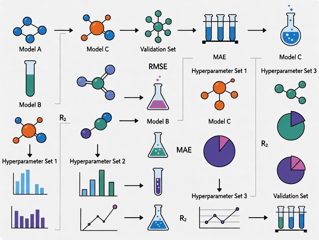
Hyperparameter Optimization Workflow: This diagram illustrates the three primary optimization methods compared in chemical ML applications, showing distinct approaches for efficient parameter tuning.
Research Infrastructure and Data Management
Effective ML implementation in chemistry requires robust data infrastructure and specialized software solutions.
FAIR Data Infrastructure for Chemical ML
The HT-CHEMBORD (High-Throughput Chemistry Based Open Research Database) project exemplifies modern research data infrastructure (RDI) designed specifically for ML-ready chemical data [1]:
Key Components:
- Automated Synthesis Platforms: Chemspeed systems for programmable chemical synthesis with parameter logging
- Multi-stage Analytical Workflow: LC-DAD-MS-ELSD-FC, GC-MS, SFC-DAD-MS-ELSD for comprehensive characterization
- Semantic Data Modeling: Converts experimental metadata to Resource Description Framework (RDF) using ontology-driven models
- Standardized Data Formats: ASM-JSON, JSON, or XML formats depending on analytical method
FAIR Principles Implementation:
- Findability: Rich metadata indexed in searchable front-end interface
- Accessibility: Controlled data access through licensing agreements
- Interoperability: Mapping to structured ontologies incorporating Allotrope Foundation Ontology
- Reusability: Detailed, standardized metadata with clear provenance
Chemical Data Analysis Pipeline: This workflow shows the automated, multi-stage process for chemical data generation and analysis, highlighting decision points that ensure comprehensive data capture including negative results.
Essential Software Solutions for Chemical ML
Table 3: Key Software Platforms for ML-Driven Chemical Research
| Software Platform | Primary Application | Key ML Features | Licensing Model | Reference |
|---|---|---|---|---|
| Schrödinger | Quantum Mechanics & Free Energy | DeepAutoQSAR, GlideScore | Modular | [9] |
| deepmirror | Hit-to-Lead Optimization | Generative AI Engine | Single Package | [9] |
| Chemaxon | Compound Design | Plexus Suite, Design Hub | Pay-per-use | [9] |
| Cresset | Protein-Ligand Modeling | Free Energy Perturbation (FEP) | Modular | [9] |
| BIOVIA | Molecular Modeling | AI-powered data analysis | Enterprise | [10] |
| Benchling | Biopharma R&D | AI-powered data insights | Subscription | [10] |
The Scientist's Toolkit: Essential Research Reagents and Solutions
Implementing ML-driven chemical research requires both computational and experimental resources:
Table 4: Essential Research Reagents and Solutions for ML-Chemistry Integration
| Reagent/Solution | Function | Application Example | Reference |
|---|---|---|---|
| Morgan Fingerprints | Molecular representation | Capturing structural features for odor prediction | [5] |
| SMILES Strings | Chemical structure encoding | Input for graph neural networks | [2] |
| Allotrope Foundation Ontology | Semantic data modeling | Standardizing experimental metadata | [1] |
| ASM-JSON Format | Analytical data storage | Instrument output standardization | [1] |
| RDKit Library | Molecular descriptor calculation | Feature extraction for QSAR models | [5] |
| Purchasable Building Blocks | Synthetic feasibility constraint | Ensuring tractable generative designs | [2] |
Machine learning has fundamentally transformed scalable chemical data analysis, enabling researchers to extract meaningful insights from increasingly large and complex datasets. Through comparative analysis of methods and applications, several key principles emerge:
First, model performance is highly dependent on appropriate molecular representations, with Morgan fingerprints demonstrating particular efficacy for sensory property prediction [5]. Second, hyperparameter optimization methods show domain-specific strengths, with Bayesian Optimization generally providing the best balance of performance and efficiency for chemical applications [7]. Third, successful ML implementation requires robust data infrastructure that adheres to FAIR principles and captures both positive and negative results [1].
Looking forward, several trends will shape the future of ML in chemical data analysis: increased integration of generative AI for molecular design [2], broader adoption of equivariant neural networks that respect physical symmetries [2], development of autonomous experimentation systems [1], and improved multi-omics data integration for drug discovery [9]. As these technologies mature, they will further accelerate the transition from data-rich to knowledge-rich chemical research, enabling more efficient discovery across pharmaceuticals, materials, and sustainable chemistry.
In the fields of cheminformatics and drug discovery, Graph Neural Networks (GNNs) have emerged as a powerful tool for molecular property prediction, drug-target interaction analysis, and reaction yield forecasting. Unlike traditional neural networks that process grid-like data, GNNs operate directly on graph-structured data, making them particularly suited for representing molecular structures where atoms serve as nodes and chemical bonds as edges. However, the performance of GNNs is highly sensitive to architectural choices and hyperparameters, making optimal configuration selection a non-trivial task that significantly impacts model accuracy, generalizability, and computational efficiency [11]. This sensitivity stems from multiple factors, including the fundamental trade-offs between different GNN architectures' expressive power, the complex interplay between hyperparameters, and the specific characteristics of chemical datasets, which are often smaller than typical deep learning benchmarks [12].
The challenge is particularly pronounced in chemistry applications, where researchers must navigate competing priorities: model expressiveness must be balanced against risks of overfitting on limited datasets, computational constraints must be considered alongside prediction accuracy requirements, and interpretability needs must be addressed without sacrificing performance. Understanding these configuration sensitivities is essential for researchers aiming to deploy GNNs effectively in molecular property prediction, drug discovery, and materials science applications [13].
Core Architectural Factors Influencing GNN Performance
Aggregation Mechanisms and Expressive Power
The core operation in GNNs is message passing, where information is aggregated from neighboring nodes to update each node's representation. The choice of aggregation function fundamentally impacts a GNN's discriminative power:
Sum aggregation provides injective multiset functions, enabling GNNs to distinguish different neighborhood structures. This approach is employed by Graph Isomorphism Networks (GINs), which achieve maximal expressive power within the conventional neighborhood aggregation paradigm, matching the ability of the 1-dimensional Weisfeiler-Lehman (1-WL) isomorphism test to distinguish non-isomorphic graphs [14].
Mean and max aggregation are not injective for multisets and can collapse non-isomorphic structures into identical embeddings. For instance, while Graph Convolutional Networks (GCNs) use mean aggregation, and some GraphSAGE variants employ max pooling, these approaches cannot capture fine-grained structural differences as effectively as sum aggregation [14].
The theoretical expressiveness directly translates to practical performance differences. In molecular classification tasks, GINs consistently achieve state-of-the-art or tied results on various benchmarks, including bioinformatics datasets like MUTAG (≈89%), PROTEINS (≈76%), and social networks like IMDB-BINARY (≈75%) [14]. However, this superior expressiveness comes with a cost: GINs require careful hyperparameter tuning and regularization, particularly in data-scarce regimes where they may be outperformed by less expressive but more stable architectures like GATs [14].
Attention Mechanisms and Neighborhood Prioritization
Graph Attention Networks (GATs) introduce attention mechanisms that assign differentiable weights to neighboring nodes during aggregation, allowing the model to focus on more relevant neighbors [15]. This dynamic weighting is particularly valuable in molecular graphs where certain atomic interactions exert stronger influence on molecular properties than others. However, the introduction of attention mechanisms adds additional parameters that require optimization and increases computational complexity [16].
The Message Passing Neural Network (MPNN) framework provides a generalized approach to message passing that encompasses many GNN variants. In comparative studies on cross-coupling reaction yield prediction, MPNNs achieved the highest predictive performance with an R² value of 0.75 across diverse datasets encompassing various transition metal-catalyzed reactions including Suzuki, Sonogashira, and Buchwald-Hartwig couplings [17]. This superior performance suggests that the flexible message functions and update mechanisms in MPNNs are particularly well-suited for capturing complex relationships in chemical reaction data.
Architectural Depth and Oversmoothing
Unlike convolutional neural networks for images, which benefit from substantial depth, most message-passing GNNs suffer from the oversmoothing problem – where node representations become indistinguishable as the number of layers increases [18]. This phenomenon fundamentally limits the effective depth of GNNs and varies in impact across architectures.
Table: Comparison of GNN Architectures and Their Sensitivity to Depth
| Architecture | Recommended Layers | Oversmoothing Sensitivity | Mitigation Strategies |
|---|---|---|---|
| GIN | 2-7 [14] | High with excessive stacking | Deeper MLPs within layers, jumping knowledge connections |
| GCN | 2-5 | Very high | Residual connections, dense connections |
| GAT | 2-5 | Moderate | Attention-guided neighborhood prioritization |
| DenseGNN | 5+ [18] | Low | Dense connectivity networks, hierarchical residual networks |
Novel architectures like DenseGNN address the depth limitation through Dense Connectivity Networks (DCN) and hierarchical node-edge-graph residual networks (HRN), enabling deeper GNNs without performance degradation [18]. This approach allows for more direct and dense information propagation throughout the network, reducing information loss during message passing and effectively combating oversmoothing. On several benchmark datasets including JARVIS-DFT, Materials Project, and QM9, DenseGNN achieved state-of-the-art performance while supporting substantially deeper architectures than conventional GNNs [18].
Hyperparameter Sensitivity and Optimization Strategies
Critical Hyperparameters and Their Impact
GNN performance depends on the careful configuration of numerous hyperparameters, each exhibiting complex interactions:
Learning Rate: Optimal values typically range between 0.01-0.02 for GINs, with Adagard often outperforming Adam optimizers in molecular property prediction tasks [14].
Embedding Dimension: Typical values range from 32-128 atoms, with higher dimensions increasing model capacity but also raising overfitting risks, particularly on small datasets [14].
MLP Depth within GIN Layers: Deeper MLPs (2-5 layers) within each GIN layer often yield more benefit than simply stacking more GIN layers [14].
Batch Normalization and Dropout: Essential for stabilizing training, especially for expressive models like GINs in small-data regimes [14].
The sensitivity of these hyperparameters is exacerbated by the characteristics of molecular datasets, which are often far smaller than typical deep learning benchmarks in other domains [12]. This data scarcity amplifies the variance introduced by suboptimal hyperparameter choices and necessitates careful regularization strategies.
Hyperparameter Optimization Methods
Given the multidimensional hyperparameter space and expensive evaluation costs, systematic Hyperparameter Optimization (HPO) is essential. Research has compared several HPO methods specifically for GNNs in molecular property prediction:
Table: Comparison of Hyperparameter Optimization Methods for GNNs
| Method | Key Principle | Strengths | Limitations |
|---|---|---|---|
| Random Search (RS) | Random sampling of hyperparameter space [12] | Good baseline, parallelizable | Inefficient for high-dimensional spaces |
| Tree-structured Parzen Estimator (TPE) | Sequential model-based optimization [12] | Efficient for limited budgets | Can get stuck in local minima |
| Covariance Matrix Adaptation Evolution Strategy (CMA-ES) | Evolutionary strategy [12] | Effective for ill-conditioned problems | Higher computational overhead |
No single HPO method dominates across all molecular tasks. Experimental studies on MoleculeNet benchmarks indicate that RS, TPE, and CMA-ES each have individual advantages for tackling different specific molecular problems [12]. The optimal choice depends on factors including dataset size, molecular complexity, and computational budget.
Experimental Protocols and Performance Benchmarking
Standardized Evaluation Methodologies
Robust evaluation of GNN configurations requires standardized protocols across several dimensions:
Dataset Partitioning: Molecular datasets are typically split using scaffold splitting, which groups molecules based on their Bemis-Murcko scaffolds, ensuring that structurally different molecules appear in training and test sets. This approach provides a more challenging and realistic assessment of generalization compared to random splitting [16].
Evaluation Metrics: Appropriate metrics must be selected based on task type:
- Regression Tasks (e.g., yield prediction, solubility): Mean Absolute Error (MAE), Root Mean Squared Error (RMSE), and R² [15]
- Classification Tasks (e.g., toxicity prediction): ROC-AUC, PRC-AUC, Balanced Accuracy [15]
- Generation Tasks (e.g., molecule generation): Validity, Uniqueness, Novelty, Quantitative Estimation of Drug-likeness (QED) [15]
Benchmark Datasets: Commonly used benchmarks include:
- MoleculeNet collections (ESOL, FreeSolv, Lipophilicity, Tox21) [15]
- Chemical Reaction Datasets encompassing various coupling reactions [17]
- Material Project datasets for crystal property prediction [18]
The following diagram illustrates a typical experimental workflow for evaluating GNN configurations in chemical applications:
Quantitative Performance Comparisons
Experimental studies consistently demonstrate significant performance variations across GNN architectures:
Table: GNN Architecture Performance on Chemical Tasks
| Architecture | Reaction Yield Prediction (R²) | Molecular Classification (AUC) | QSAR Regression (MAE) | Computational Cost |
|---|---|---|---|---|
| MPNN | 0.75 [17] | - | - | Medium |
| GIN | - | 0.793-0.849 [14] | 0.44 [14] | High |
| GAT | - | Moderate [14] | - | Medium-High |
| GCN | - | Lower than GIN [14] | - | Low |
| ECFP-MLP | - | - | 0.42 [14] | Low |
The performance hierarchy varies substantially across task types. For reaction yield prediction on heterogeneous datasets encompassing various cross-coupling reactions, MPNNs achieve superior performance [17]. For molecular classification tasks on toxicological assays, GINs typically outperform GCNs and GATs in data-rich environments [14]. However, in quantitative structure-activity relationship (QSAR) regression, classical ECFP-MLP baselines can sometimes outperform GIN-based models, highlighting that the optimal architecture is highly task-dependent [14].
Implementing and optimizing GNNs for chemical applications requires leveraging specialized tools, datasets, and methodologies:
Table: Essential Research Reagents for GNN Experimentation
| Resource Category | Specific Examples | Function | Access/Implementation |
|---|---|---|---|
| Molecular Datasets | ESOL, FreeSolv, Lipophilicity, Tox21 [15] | Benchmark performance across chemical domains | MoleculeNet |
| Chemical Features | Circular Atomic Features [16], Daylight atomic invariants [16] | Enhanced node/edge representations for molecules | RDKit, DeepChem |
| HPO Algorithms | TPE, CMA-ES, Random Search [12] | Efficient navigation of hyperparameter space | Optuna, Scikit-optimize |
| Interpretability Methods | GNNExplainer, Integrated Gradients [16] | Identify salient molecular substructures and features | PyTorch Geometric |
| Architecture Variants | DenseGNN, ALIGNN, GIN, MPNN [18] [17] [14] | Address specific limitations like oversmoothing | Various GitHub repositories |
The performance sensitivity of GNNs to their configuration is not merely an implementation challenge but stems from fundamental architectural trade-offs. The most expressive architectures (e.g., GINs) typically require the most careful regularization and hyperparameter tuning, particularly in the data-scarce environments common in chemical research. Meanwhile, architectures with inherent constraints may offer more stable performance at the cost of representational power.
Successful deployment of GNNs in chemical applications requires a methodical approach: (1) establishing clear performance requirements and constraints, (2) selecting architectures aligned with both data characteristics and task objectives, (3) implementing systematic hyperparameter optimization informed by dataset size and complexity, and (4) incorporating interpretability techniques to validate model behavior against chemical intuition.
As the field evolves, emerging techniques including automated Neural Architecture Search (NAS), self-supervised pretraining strategies, and novel architectures that explicitly balance expressiveness with stability are poised to reduce the configuration burden while maintaining performance. However, understanding the fundamental sources of configuration sensitivity will remain essential for researchers aiming to leverage GNNs effectively in drug discovery, materials science, and chemical synthesis prediction.
Defining Hyperparameter Optimization (HPO) and Neural Architecture Search (NAS)
In the competitive landscape of modern computational research, particularly in chemistry and drug development, the manual design and tuning of machine learning models are no longer sufficient. The pursuit of higher accuracy, greater efficiency, and more interpretable models has given rise to Automated Machine Learning (AutoML). Two core pillars of AutoML are Hyperparameter Optimization (HPO) and Neural Architecture Search (NAS). While often mentioned together, they address distinct aspects of the model creation process. This guide provides a definitive comparison of HPO and NAS, framing them within the context of chemistry model research. We will dissect their definitions, methodologies, and practical applications, supported by experimental data and protocols relevant to scientists and researchers in drug discovery.
Core Definitions and Comparative Framework
What is Hyperparameter Optimization (HPO)?
Hyperparameter Optimization (HPO) is the automated process of finding the optimal set of hyperparameters for a given machine learning algorithm. Hyperparameters are configuration settings that are not learned from the data but are set prior to the training process. They control the learning process itself, such as the learning rate, the number of layers in a neural network, or the batch size. The goal of HPO is to find the combination of these settings that results in the best model performance, typically measured by accuracy or another relevant metric on a validation set [19] [20]. In essence, HPO tunes the "knobs" of a fixed model architecture.
What is Neural Architecture Search (NAS)?
Neural Architecture Search (NAS) is the automated process of designing the architecture of a neural network. Instead of just tuning the parameters of a fixed structure, NAS searches for the structure itself. This involves making fundamental decisions about the network's composition, such as the types of operations (e.g., convolution, pooling, attention), how they are connected (e.g., sequential, residual, branching), and the overall depth and width of the network [11] [21]. NAS automates the design of the model's blueprint, a task that traditionally requires significant human expertise and trial and error.
HPO vs. NAS: A Side-by-Side Comparison
The table below summarizes the key distinctions between HPO and NAS.
Table 1: Fundamental Comparison Between HPO and NAS
| Aspect | Hyperparameter Optimization (HPO) | Neural Architecture Search (NAS) |
|---|---|---|
| Primary Goal | Tune the settings of a fixed model architecture [21]. | Find the optimal model structure itself [21]. |
| What is Searched | Learning rate, number of epochs, optimizer type, batch size, number of neurons in a fixed layer [20] [19]. | Types of layers (convolution, pooling), connectivity patterns (skip connections), number of layers [11] [21]. |
| Search Space | Often a predefined set of values or ranges for specific parameters. | A space of possible neural network architectures, often represented as a directed acyclic graph (DAG) [21]. |
| Typical Scope | A component of the model training process. | Encompasses model design and can include HPO within its process. |
| Computational Cost | Can be high, but generally lower than NAS. | Often very high, though advanced methods like weight-sharing aim to reduce this [21]. |
Diagram 1: HPO and NAS Decision Flow
Key Methodologies and Experimental Protocols
The effectiveness of HPO and NAS hinges on the strategies used to navigate their respective search spaces. The following section details common optimization methods and experimental frameworks.
Common HPO and NAS Search Strategies
Researchers and engineers employ various strategies to automate the search for optimal configurations.
Table 2: Comparison of Primary Search Strategies
| Search Strategy | Description | Typical Use Case |
|---|---|---|
| Grid Search | An exhaustive search that tests all possible combinations of hyperparameter values within a predefined set. It is guaranteed to find the best combination within the grid but is computationally very expensive [19]. | HPO with a small, well-defined search space. |
| Random Search | Randomly selects hyperparameter combinations from a defined range. It is more efficient than grid search and often finds good solutions faster, as it does not waste resources on evaluating every single combination [19]. | HPO with a larger search space where computational budget is limited. |
| Bayesian Optimization | A sequential model-based optimization technique. It uses the results of past evaluations to build a probabilistic model of the objective function and selects the next hyperparameters to evaluate that are most likely to improve performance [19]. | Both HPO and NAS for efficient search in complex, expensive-to-evaluate spaces. |
| Max-Flow Based Search (MF-NAS/MF-HPO) | A novel approach that formulates the search for an optimal architecture or hyperparameters as a max-flow problem on a graph. The "capacity" of edges represents the importance of different operations or hyperparameter intervals, guiding the search efficiently [21]. | NAS and HPO, particularly when the search space can be naturally represented as a graph. |
Diagram 2: Generic Search Strategy Workflow
Experimental Protocol: HPO for Chemical Reaction Prediction
A practical example of HPO in chemistry research comes from a study optimizing a neural network to predict coefficients for the decay plots of Methylene Blue (MB) absorbance during its reduction by Ascorbic Acid [22].
Objective: To predict the coefficients (A, B, C) in the exponential decay equation A + B · e^(-x/C) that describes the reduction reaction of Methylene Blue.
Methodology:
- Data Collection: 220 spectral files were obtained from reactions with varying concentrations of MB, Ascorbic Acid, and solvents. After filtering, 180 records were used for training.
- HPO Setup: A grid search was employed to explore the hyperparameter space.
- Search Space:
- Number of hidden layers: 1 to 5
- Number of neurons per layer: 16 to 256
- Activation function: ReLU, Sigmoid, Tanh, Leaky ReLU, ELU, Swish
- Training epochs: 50 or 100
- Batch size: Varied
Result: The optimal architecture identified was a network with five hidden layers, each containing sixteen neurons, and using the Swish activation function. This model achieved low normalized mean square errors (NMSE) for predicting the decay coefficients [22].
Experimental Protocol: NAS and Novel Architecture Design in Cheminformatics
NAS is increasingly used to develop novel, high-performing model architectures for molecular property prediction, a key task in drug discovery.
Objective: Design a Graph Neural Network (GNN) that surpasses the performance of manually designed architectures for molecular property prediction.
Methodology (KA-GNN):
- Search Space Definition: The search space integrates Kolmogorov-Arnold Networks (KANs) into the fundamental components of a GNN: node embedding, message passing, and readout [23].
- Architectural Innovation: The proposed KA-GNN replaces standard multi-layer perceptrons (MLPs) in GNNs with Fourier-series-based KAN modules. This enhances the model's ability to capture complex, non-linear patterns in molecular graph data [23].
- Evaluation: Two variants, KA-GCN and KA-GAT, were developed and evaluated across seven benchmark molecular datasets.
Result: The NAS-derived KA-GNN architectures consistently outperformed conventional GNNs in both prediction accuracy and computational efficiency. They also offered improved interpretability by highlighting chemically meaningful molecular substructures [23].
Performance Data and Comparison
The true value of HPO and NAS is demonstrated through quantitative performance gains. The table below summarizes key results from the cited experiments.
Table 3: Experimental Performance Comparison
| Experiment | Method | Key Performance Metric | Result | Comparative Outcome |
|---|---|---|---|---|
| Chemical Reaction Prediction [22] | HPO (Grid Search) | Normalized Mean Square Error (NMSE) | NMSE of 0.05, 0.03, and 0.04 for coefficients A, B, and C, respectively. | A 5-layer Swish network was optimal. |
| Molecular Property Prediction [23] | NAS (KA-GNN) | Prediction Accuracy & Efficiency | Consistently higher accuracy and better computational efficiency across 7 molecular benchmarks. | Outperformed conventional GNNs (GCN, GAT). |
| General AutoML [21] | MF-NAS / MF-HPO | Search Efficacy & Efficiency | Competitive results across diverse datasets and search spaces. | Matched or exceeded state-of-the-art methods. |
The Scientist's Toolkit: Essential Research Reagents and Materials
For researchers looking to replicate or build upon HPO and NAS experiments in chemistry, the following tools and "reagents" are essential.
Table 4: Key Research Reagents and Solutions for HPO/NAS Experiments
| Item / Tool | Function / Description | Example Use in Context |
|---|---|---|
| Benchmark Datasets | Standardized datasets used to evaluate and compare model performance fairly. | Molecular datasets (e.g., from MoleculeNet) for drug discovery [11]; ImageNet for computer vision [24]. |
| HPO/NAS Frameworks | Software libraries that automate the search process. | Optuna, HyperOpt, Ray Tune for HPO [20]; frameworks supporting DARTS or weight-sharing for NAS. |
| Graph Neural Network (GNN) | A deep learning model that operates directly on graph-structured data. | The base model for molecular property prediction, as molecules are naturally represented as graphs [11] [23]. |
| Methylene Blue (MB) & Ascorbic Acid (AA) | Chemical reagents in a model reaction system for kinetic studies. | Used to generate spectroscopic data for training the HPO-tuned neural network in [22]. |
| Spectrophotometer | An instrument that measures the absorption of light by a chemical substance. | Used to track the concentration of Methylene Blue over time by measuring absorbance at λ=665 nm [22]. |
In the field of chemical and molecular informatics, machine learning models are increasingly employed for critical tasks such as molecular property prediction, toxicity classification, and de novo molecular design. The performance of these models is highly sensitive to their hyperparameters—the configuration variables that govern the learning process itself. Hyperparameter optimization (HPO) is the systematic process of finding the optimal set of these hyperparameters to maximize model performance on a given task. However, HPO presents significant challenges in computational cost, scalability, and navigating the curse of dimensionality, particularly when dealing with the high-dimensional feature spaces common in chemical data. The curse of dimensionality refers to various phenomena that arise when analyzing data in high-dimensional spaces, including increased computational complexity and the counterintuitive nature of geometric relationships, which severely impact the performance of machine learning algorithms [25] [26].
This guide provides a comprehensive comparison of HPO methods specifically within the context of chemistry models, evaluating their performance against quantitative metrics and providing detailed experimental protocols. As the complexity of chemical datasets and models continues to grow, selecting an appropriate HPO strategy becomes paramount for researchers aiming to develop accurate, efficient, and scalable machine learning solutions for drug discovery and materials science.
Theoretical Foundations: The HPO Problem and Its Challenges
Defining the Hyperparameter Optimization Problem
In supervised machine learning, an algorithm ingests training data and outputs a predictor. The quality of this predictor is measured on validation data using an evaluation metric, such as error rate or accuracy. Since the predictor depends on the chosen hyperparameters, the validation performance also depends on those hyperparameters. The mapping from hyperparameter values to validation performance is termed the response function. HPO consists of finding the hyperparameters that optimize this response function [27].
The HPO problem is distinguished from conventional optimization by its nested structure: evaluating the response function for a given hyperparameter configuration requires executing the learning algorithm, which typically involves solving another optimization problem to fit a model to the training data. This characteristic means the response function is rarely available in closed form and is often stochastic, non-convex, and computationally expensive to evaluate—sometimes requiring hours or days of computation for a single configuration [27].
Key Challenges in High-Dimensional Spaces
The curse of dimensionality manifests in HPO through several interconnected challenges. As the number of hyperparameters increases, the search space grows exponentially, a phenomenon known as combinatorial explosion. For example, if each of 10 hyperparameters has just 5 possible values, the total number of combinations exceeds 10 million. This exponential growth makes exhaustive search strategies computationally infeasible [27] [26].
High-dimensional spaces also exhibit sparse sampling; data points tend to reside in the corners of the space rather than the center, and distance measures become less meaningful as dimensionality increases. These factors severely impact the performance of machine learning models applied to chemical data, such as molecular fingerprints, which are inherently high-dimensional [25]. Additionally, the hyperparameter search space is often complex and heterogeneous, containing continuous, integer, and categorical variables, some of which may only be relevant conditionally based on the values of others [27].
Comparative Analysis of Hyperparameter Optimization Methods
Traditional HPO Methods
Grid Search exhaustively explores a predefined set of hyperparameter values. For example, when tuning a Random Forest with three hyperparameters (nestimators, maxdepth, minsamplessplit), each with three possible values, Grid Search would train and evaluate 3×3×3=27 separate models [28]. While thorough, this approach becomes computationally prohibitive as the number of hyperparameters increases, failing to leverage information from previous evaluations.
Random Search randomly samples a fixed number of hyperparameter configurations from specified distributions. Rather than trying all combinations, it selects random combinations, which can be more efficient, especially with many parameters or large ranges. However, it performs a blind search with no learning from previous trials and may miss optimal configurations due to its random nature [28].
Bayesian Optimization and Modern Frameworks
Bayesian Optimization represents a more intelligent approach that builds a probabilistic model of the objective function to guide the search process efficiently. The core components include a surrogate model, typically a Gaussian Process or Tree-structured Parzen Estimator (TPE), which approximates the unknown objective function, and an acquisition function that determines the next hyperparameters to evaluate by balancing exploration and exploitation [28] [29].
Optuna is a powerful HPO framework that implements Bayesian optimization with several enhancements. It employs a "define-by-run" API that allows users to dynamically construct the search space and uses TPE for modeling the objective function. Optuna also incorporates pruning to automatically terminate unpromising trials early, significantly reducing computational waste [28].
Table 1: Comparison of Hyperparameter Optimization Methods
| Method | Search Strategy | Scalability | Best For | Key Limitations |
|---|---|---|---|---|
| Grid Search | Exhaustive search over predefined grid | Poor with high-dimensional spaces | Small search spaces with few hyperparameters | Computationally expensive; fails to leverage past evaluations |
| Random Search | Random sampling from distributions | Moderate improvement over Grid Search | Medium-dimensional spaces with limited budget | Blind search; may miss optima; performance depends on luck |
| Bayesian Optimization (e.g., Optuna) | Sequential model-based optimization using surrogate models and acquisition functions | Excellent for high-dimensional, complex spaces | Expensive black-box functions with complex search spaces | Overhead of maintaining model; can over-exploit |
Experimental Protocols and Performance Benchmarks
Protocol for Bayesian Optimization
A standardized protocol for implementing Bayesian Optimization with Optuna involves several key steps [28] [29]:
- Define the Objective Function: Create a function that takes a set of hyperparameters, builds and trains a model with those hyperparameters, and returns a validation performance metric.
- Configure the Tuner: Initialize the Bayesian optimization tuner, specifying parameters such as the number of initial random points and the total number of trials.
- Execute the Search: Run the optimization process, where the algorithm selects hyperparameters, evaluates them, and updates its probabilistic model.
- Retrieve Results: Extract the best-performing hyperparameters and the corresponding model.
Diagram Title: Bayesian Optimization Workflow
Quantitative Performance Comparison
In practical applications, Bayesian optimization consistently outperforms traditional methods. In a fraud detection case study, Bayesian optimization successfully tuned a deep learning model, significantly improving recall from 0.66 to 0.84, though with expected trade-offs in precision and accuracy [29].
Table 2: Performance Comparison of HPO Methods on Model Tuning Tasks
| Method | Best Validation Recall | Computational Time (Relative) | Number of Trials to Convergence | Key Hyperparameters Identified |
|---|---|---|---|---|
| Grid Search | 0.745 | 100% (baseline) | ~200 (exhaustive) | Fixed grid values |
| Random Search | 0.792 | ~65% | ~130 | Random sampling |
| Bayesian Optimization (Optuna) | 0.840 | ~45% | ~75 | neurons1: 40, dropoutrate2: 0.4, learningrate: 0.004 |
For chemical domain tasks, a study comparing embedding techniques for toxicity classification provides further evidence. When optimizing classifiers on different molecular representations, models leveraging modern HPO techniques demonstrated superior performance across multiple toxicity endpoints, with Matthews Correlation Coefficient values improving by 0.1-0.3 compared to baseline methods [25].
Specialized Applications in Chemical Informatics
Combating Dimensionality in Molecular Representation
Chemical datasets often suffer from extreme dimensionality, particularly when using molecular fingerprints or descriptor-based representations. Dimensionality reduction techniques serve as crucial preprocessing steps to mitigate the curse of dimensionality before model training and HPO. Principal Component Analysis provides a linear transformation that maximizes variance explanation but may miss nonlinear relationships. Uniform Manifold Approximation and Projection is a nonlinear method that utilizes local manifold approximations and topological representations. Variational Autoencoders employ deep learning to learn compressed representations in an unsupervised manner, often demonstrating advantages in maintaining chemical information [25].
In toxicity classification benchmarks, using VAE embeddings as features for optimized classifiers consistently showed advantages in accuracy over PCA and UMAP approaches, particularly for complex toxicity endpoints like NR-AR and NR-AR-LBD, where VAE-based models achieved MCC values above 0.60 [25].
Advanced Architectures for High-Dimensional Problems
Novel neural architectures specifically designed for high-dimensional problems have emerged recently. Anant-Net addresses the curse of dimensionality in solving high-dimensional partial differential equations by using tensor product structures and dimension-wise sweeps. This approach efficiently incorporates boundary conditions and minimizes PDE residuals at collocation points, successfully solving PDEs up to 300 dimensions on a single GPU [30] [26].
For molecular systems, AlphaNet represents a local-frame-based equivariant model for interatomic potentials that achieves both computational efficiency and predictive precision. By constructing equivariant local frames with learnable geometric transitions, AlphaNet enhances representational capacity while maintaining scalability across diverse system sizes [31].
The Scientist's Toolkit: Essential Research Reagents
Table 3: Essential Tools for Hyperparameter Optimization in Chemistry Research
| Tool Name | Type | Primary Function | Application in Chemistry Models |
|---|---|---|---|
| Optuna | Hyperparameter Optimization Framework | Implements Bayesian optimization with pruning and dynamic search spaces | Tuning neural networks for molecular property prediction and toxicity classification |
| Scikit-learn | Machine Learning Library | Provides implementations of GridSearchCV and RandomizedSearchCV | Baseline HPO for traditional QSAR models using random forests and SVMs |
| KerasTuner | Deep Learning HPO Library | Bayesian optimization for Keras/TensorFlow models | Architecture search for deep neural networks processing chemical structures |
| RDKit | Cheminformatics Library | Generates molecular fingerprints and descriptors | Creates high-dimensional features from molecular structures that require optimization |
| Dimensionality Reduction | Preprocessing | Techniques like PCA, UMAP, VAE to reduce feature space | Compresses molecular fingerprints before model training to mitigate curse of dimensionality |
The effective optimization of hyperparameters presents significant challenges in computational cost, scalability, and navigating the curse of dimensionality, particularly for chemistry models operating on high-dimensional molecular representations. Traditional methods like Grid Search and Random Search provide baseline approaches but become computationally prohibitive as model complexity increases. Bayesian optimization frameworks like Optuna offer substantial improvements in efficiency and effectiveness by leveraging probabilistic models to guide the search process intelligently.
When combined with dimensionality reduction techniques and specialized neural architectures, modern HPO methods enable researchers to develop more accurate and scalable models for chemical informatics tasks. As the field advances, the integration of these approaches will be crucial for tackling increasingly complex problems in drug discovery and materials science, where both data dimensionality and model complexity continue to grow exponentially.
A Deep Dive into HPO Algorithms: From Bayesian Optimization to Evolutionary Strategies
Bayesian Optimization (BO) is a powerful machine learning approach for finding the global optimum of black-box functions that are expensive, difficult, or noisy to evaluate [32] [33]. This makes BO particularly valuable for scientific and engineering applications where each function evaluation consumes substantial computational resources or requires physical experiments. In chemistry and drug discovery, BO has emerged as a transformative technology, enabling researchers to navigate complex experimental spaces—such as chemical synthesis parameters or molecular combinations—with dramatically fewer experiments than traditional approaches [34] [35] [36].
Unlike gradient-based optimization methods that require derivative information, BO constructs a probabilistic surrogate model of the objective function and uses an acquisition function to guide the search process [33] [37]. This sequential model-based optimization strategy is especially effective for problems with high-dimensional parameter spaces and costly evaluations, which are common in hyperparameter tuning for chemistry models and drug discovery pipelines [34] [35].
Core Principles of Bayesian Optimization
The Bayesian Optimization Framework
At its core, Bayesian Optimization operates on the principle of iterative refinement. The algorithm begins with an initial set of observations and progressively selects new evaluation points that balance exploration of uncertain regions with exploitation of known promising areas [37]. This process is formalized through Bayes' theorem, which describes the correlation between different events and enables the calculation of conditional probabilities [34]. The BO framework can be summarized as follows [34] [33]:
- Initialization: Start with a small set of initial observations of the objective function.
- Surrogate Modeling: Build a probabilistic surrogate model that approximates the objective function.
- Acquisition: Use an acquisition function to determine the most promising point to evaluate next.
- Evaluation: Evaluate the objective function at the selected point.
- Update: Incorporate the new observation into the surrogate model.
- Iteration: Repeat steps 2-5 until convergence or budget exhaustion.
The Exploration-Exploitation Tradeoff
A fundamental principle underlying BO is the exploration-exploitation tradeoff [37]. Exploitation involves sampling areas where the surrogate model predicts high performance, while exploration targets regions with high uncertainty where surprising improvements might be found [33] [37]. The acquisition function quantitatively balances these competing objectives, ensuring the algorithm neither converges prematurely to local optima nor wastes excessive resources on unpromising regions of the search space [37].
Surrogate Models in Bayesian Optimization
Gaussian Process Regression
The Gaussian Process (GP) is the most widely used surrogate model in Bayesian Optimization [32] [38]. A GP defines a distribution over functions, where any finite collection of function values follows a multivariate Gaussian distribution [38]. Formally, a Gaussian Process is fully specified by a mean function μ(·) and a kernel function K(·, ·):
f(·) ∼ GP(μ(·), K(·, ·))
The mean function is often set to zero or a constant, while the kernel function encodes assumptions about the function's smoothness and continuity [38]. Through Bayesian inference, the GP posterior distribution provides both mean predictions and uncertainty estimates for unseen data points, which is crucial for the acquisition function's decision-making process [33] [38].
Table 1: Common Kernel Functions in Gaussian Processes
| Kernel Name | Mathematical Form | Key Properties |
|---|---|---|
| Radial Basis Function (RBF) | ( k{\text{RBF}}(\bm{x},\bm{x}') = \theta{\text{out}}\exp\left(-\frac{1}{2}r(\bm{x}, \bm{x}')\right) ) | Infinitely differentiable, produces smooth functions |
| Matérn | ( k\nu(\bm{x}, \bm{x}') = \theta{\text{out}}\frac{2^{1 - \nu}}{\Gamma(\nu)}(\sqrt{2\nu}r)^\nu K_\nu(\sqrt{2\nu}r) ) | More flexible than RBF, with parameter ν controlling smoothness |
Alternative Surrogate Models
While Gaussian Processes are the standard choice for BO, other surrogate models can be employed, particularly in high-dimensional settings or with large datasets:
- Random Forests: Often used in the Sequential Model-Based Algorithm Configuration (SMAC) framework, random forests can handle categorical parameters more naturally than GPs [39].
- Bayesian Neural Networks: These provide greater scalability to high dimensions and large datasets, though they can be more complex to implement and train [32].
Acquisition Functions
Acquisition functions are the decision-making engine of Bayesian Optimization, quantifying the potential utility of evaluating different points in the search space [33]. They use the surrogate model's predictions to balance exploration and exploitation [37].
Common Acquisition Functions
Table 2: Comparison of Acquisition Functions
| Acquisition Function | Mathematical Form | Strengths | Weaknesses |
|---|---|---|---|
| Upper Confidence Bound (UCB) | ( a(x;\lambda) = \mu(x) + \lambda \sigma (x) ) | Simple, explicit exploration-exploitation parameter λ | Requires careful tuning of λ |
| Probability of Improvement (PI) | ( \text{PI}(x) = \Phi\left(\frac{\mu(x)-f(x^\star)}{\sigma(x)}\right) ) | Intuitive, focuses on probability of improvement | Tends to over-exploit, ignores improvement magnitude |
| Expected Improvement (EI) | ( \text{EI}(x) = \left(\mu- f(x^\star)\right) \Phi\left(\frac{\mu-f(x^\star)}{\sigma}\right) + \sigma \varphi\left(\frac{\mu - f(x^\star)}{\sigma}\right) ) | Considers both probability and magnitude of improvement | More computationally intensive than PI |
Optimization of Acquisition Functions
A critical step in the BO cycle is maximizing the acquisition function to select the next evaluation point [32]. While gradient-based methods like L-BFGS-B are commonly used, they can converge to local optima [32]. Recent research has explored mixed-integer programming (MIP) approaches that provide global optimality guarantees for acquisition function optimization [32]. The Piecewise-linear Kernel Mixed Integer Quadratic Programming (PK-MIQP) formulation, for example, introduces a piecewise-linear approximation for GP kernels and admits a corresponding MIQP representation for acquisition functions with theoretical regret bounds [32].
Performance Comparison of Optimization Methods
Comparative Studies in Healthcare and Chemistry
Multiple studies have systematically compared Bayesian Optimization against alternative hyperparameter optimization methods across different domains:
Table 3: Performance Comparison of Optimization Methods in Healthcare Applications
| Study Context | Optimization Methods | Key Performance Findings | Reference |
|---|---|---|---|
| Heart Failure Prediction | Grid Search (GS), Random Search (RS), Bayesian Search (BS) | BS had best computational efficiency; Random Forest with BS showed superior robustness with AUC improvement of 0.03815 | [8] |
| Predicting High-Need Healthcare Users | 9 HPO methods for XGBoost | All HPO methods improved AUC (0.82 to 0.84) and calibration vs. default parameters; similar gains across methods attributed to large sample size and strong signal-to-noise ratio | [39] |
| Mechanical Properties of Nanocomposites | BO, Simulated Annealing (SA), Genetic Algorithm (GA) | GA consistently outperformed BO and SA for most mechanical properties; BO achieved highest R² (0.9776) for modulus of elasticity prediction | [40] |
In chemistry and drug discovery, Bayesian Optimization has demonstrated remarkable efficiency. In one prospective study screening 206 drugs across 16 cancer cell lines, a Bayesian active learning platform (BATCHIE) accurately predicted unseen combinations and detected synergies after exploring only 4% of the 1.4 million possible experiments [36]. The platform identified a panel of effective combinations for Ewing sarcomas, including the clinically relevant combination of PARP plus topoisomerase I inhibition [36].
Multifidelity Bayesian Optimization
Multifidelity Bayesian Optimization (MF-BO) extends standard BO by incorporating information from experimental sources of differing cost and accuracy [35]. This approach mirrors the traditional experimental funnel in pharmaceutical discovery, where low-fidelity assays screen large compound libraries, and higher-fidelity assays validate promising candidates [35].
In drug discovery applications, MF-BO has been shown to outperform experimental funnels, transfer learning with low-fidelity data, and Bayesian optimization using only high-fidelity data [35]. By optimally allocating resources across docking scores (low-fidelity), single-point percent inhibitions (medium-fidelity), and dose-response IC₅₀ values (high-fidelity), MF-BO accelerates the discovery of potent drug molecules while reducing experimental costs [35].
Experimental Protocols and Methodologies
Standard Bayesian Optimization Workflow
Bayesian Optimization Workflow: This diagram illustrates the iterative process of Bayesian Optimization, showing how the surrogate model and acquisition function guide the selection of evaluation points until convergence.
Protocol for Comparative Studies
Robust experimental comparison of optimization methods requires careful protocol design. A typical methodology includes:
- Dataset Preparation: Use real-world datasets with known ground truth or well-established benchmarks [8] [35].
- Optimization Methods: Implement multiple optimization algorithms with appropriate hyperparameter spaces [8] [39].
- Evaluation Metrics: Define objective functions based on relevant performance metrics (AUC, RMSE, R², etc.) [8] [40].
- Validation: Employ cross-validation or hold-out test sets to assess generalization performance [8].
- Budgeting: Specify computational budgets (number of trials or function evaluations) for each method [39].
- Multiple Runs: Conduct multiple independent runs with different random seeds to account for stochasticity [40].
For example, in the heart failure prediction study, researchers evaluated GS, RS, and BS across SVM, RF, and XGBoost algorithms using real patient data with 167 features from 2008 patients [8]. The study implemented multiple imputation techniques for missing values and employed 10-fold cross-validation to assess model robustness [8].
The Scientist's Toolkit
Table 4: Essential Research Reagents and Computational Tools for Bayesian Optimization
| Tool Name | Type | Primary Function | Application Context |
|---|---|---|---|
| BoTorch | Software Library | Bayesian Optimization research framework with Monte Carlo acquisition functions | General-purpose BO, multi-objective optimization [32] |
| GPyTorch | Software Library | Gaussian Process modeling with GPU acceleration | Large-scale GP regression for BO [38] |
| BATCHIE | Software Platform | Bayesian active learning for combination drug screens | Adaptive design of drug combination experiments [36] |
| Optuna | Software Framework | Hyperparameter optimization with efficient sampling algorithms | Automated ML pipeline tuning [39] |
| Gaussian Process | Surrogate Model | Probabilistic function approximation with uncertainty quantification | Standard surrogate model for BO [33] [38] |
| Morgan Fingerprints | Molecular Representation | Molecular structure encoding using circular fingerprints | Chemical compound representation in drug discovery BO [35] |
Bayesian Optimization represents a powerful paradigm for optimizing expensive black-box functions, with particular relevance to chemistry and drug discovery applications. The method's strength lies in its principled balance of exploration and exploitation through acquisition functions, and its ability to quantify uncertainty through surrogate models, typically Gaussian Processes.
While comparative studies show that BO consistently outperforms simpler alternatives like Grid Search and Random Search, its performance relative to other sophisticated optimizers like Genetic Algorithms appears context-dependent [8] [40]. In scenarios with large sample sizes, low-dimensional feature spaces, and strong signal-to-noise ratios, multiple optimization methods may achieve similar performance [39]. However, BO's sample efficiency makes it particularly valuable for applications with expensive function evaluations, such as experimental chemistry and clinical prediction models.
Emerging directions in Bayesian Optimization include multifidelity approaches that leverage experiments of varying cost and accuracy [35], Bayesian active learning for large-scale experimental design [36], and improved global optimization of acquisition functions using mixed-integer programming [32]. These advances promise to further expand BO's applicability and effectiveness in chemical and pharmaceutical research.
In the field of computational intelligence, Evolutionary Algorithms (EA) provide powerful tools for solving complex optimization problems where traditional mathematical methods fall short. Among the most prominent EAs are Genetic Algorithms (GA) and Particle Swarm Optimization (PSO), which draw inspiration from different natural phenomena. GA mimics the process of natural selection and evolution, operating through selection, crossover, and mutation on a population of potential solutions. In contrast, PSO simulates social behavior, such as bird flocking or fish schooling, where particles navigate the solution space by adjusting their positions based on individual and collective experiences [41] [42].
These algorithms have found significant application in chemistry and drug discovery, where they help researchers navigate vast chemical spaces to identify compounds with desirable properties. The performance of these algorithms is highly dependent on their parameter configurations and problem-aware designs, making understanding their comparative strengths crucial for effective implementation in research settings [43] [11].
Algorithmic Fundamentals: How GA and PSO Work
Genetic Algorithm Workflow
GAs operate through a cycle inspired by biological evolution, maintaining a population of candidate solutions that undergo selective pressure and genetic operations over multiple generations [44] [41]:
- Initialization: Creating an initial population of random solutions (chromosomes)
- Evaluation: Assessing solution quality using a fitness function
- Selection: Choosing the fittest solutions as parents for reproduction
- Crossover: Combining parent solutions to create offspring
- Mutation: Introducing random changes to maintain diversity
- Replacement: Forming the next generation from parents and offspring
Particle Swarm Optimization Workflow
PSO operates through a different paradigm, where potential solutions (particles) fly through the solution space, adjusting their trajectories based on personal and collective experiences [42]:
- Initialization: Initialize particle positions and velocities randomly
- Evaluation: Calculate fitness for each particle
- Update Personal Best: Track best position encountered by each particle
- Update Global Best: Track best position found by entire swarm
- Velocity Update: Adjust velocity based on personal and global bests
- Position Update: Move particles to new positions
Position Update Mechanisms
The core PSO position update equations demonstrate how social information guides the search process [45]:
Velocity Update Equation:
Position Update Equation:
Where:
v_i(k)is particle i's velocity at iteration kx_i(k)is particle i's position at iteration kwis inertia weight controlling momentumc₁, c₂are acceleration coefficientsr₁, r₂are random numbers between 0 and 1pbest_iis particle i's personal best positiongbestis the swarm's global best position
Performance Comparison: Quantitative Analysis
Benchmark Performance Analysis
Extensive testing on standard benchmark functions reveals distinct performance characteristics for each algorithm. The following table summarizes key comparative metrics based on empirical studies:
Table 1: Performance Comparison on Standard Benchmark Functions
| Performance Metric | Genetic Algorithm (GA) | Particle Swarm Optimization (PSO) | Hybrid IGA-IPSO |
|---|---|---|---|
| Average Execution Time | 5.1059 seconds [46] | 4.5632 seconds [46] | 1.8527 seconds [46] |
| Friedman Rank | Not specified | Not specified | 1.2308 (top rank) [46] |
| Convergence Speed | Moderate [42] | Fast [42] | Fastest [46] |
| Global Search Capability | Good [41] | Good [41] | Superior [46] |
| Local Optima Avoidance | Mutation operators help escape local optima [41] | Social learning helps escape local optima [41] | Enhanced via constriction coefficient and chaotic search [46] |
Application-Specific Performance
The relative performance of GA and PSO varies significantly across application domains, with each demonstrating strengths in different contexts:
Table 2: Domain-Specific Performance Comparison
| Application Domain | Genetic Algorithm Performance | Particle Swarm Optimization Performance | Remarks |
|---|---|---|---|
| Optimal Power Flow | Slightly better accuracy [42] | Less computational burden [42] | Both offer remarkable accuracy [42] |
| High-Dimensional Feature Selection | Not specified | Superior balance between feature number and classification accuracy with PAPSO variant [43] | Problem-aware hyperparameter design crucial [43] |
| Molecular Optimization | Used in earlier de novo design approaches [47] | Effective in continuous latent spaces (Molecule Swarm Optimization) [47] | PSO enables flexible objective functions [47] |
| Stochastic Biochemical Systems | Suitable for parameter estimation [48] | More suitable for parameter estimation [48] | PSO reliably reconstructs system dynamics [48] |
Chemistry Applications: Case Studies and Experimental Protocols
Molecular Optimization with Particle Swarm Optimization
The application of PSO to molecular optimization, known as Molecule Swarm Optimization (MSO), represents a significant advancement in de novo drug design. This approach operates in a continuous latent space of chemical structures, allowing efficient navigation of the chemical landscape [47].
Experimental Protocol for MSO:
Latent Space Representation: Encode chemical structures into continuous vectors using a variational autoencoder trained on SMILES notations [47]
Swarm Initialization: Initialize particle positions randomly in the latent space, with each position decodable to a molecular structure [47]
Objective Function Definition: Define a composite objective function incorporating:
- Predicted biological activity from QSAR models
- ADME properties (solubility, metabolic stability)
- Drug-likeness metrics (QED)
- Synthetic accessibility scores
- Substructure constraints or penalties [47]
Iterative Optimization:
- Evaluate each particle's position by decoding to molecular structure and computing objective function
- Update personal best (pbest) and global best (gbest) positions
- Update particle velocities and positions using standard PSO equations [47]
Termination and Validation:
- Continue for fixed iterations or until convergence
- Validate top-ranking molecules through synthetic testing [47]
FACTS Device Optimization with Hybrid Approach
A hybrid Improved Genetic Algorithm-Improved Particle Swarm Optimization (IGA-IPSO) has demonstrated exceptional performance in optimizing Flexible AC Transmission Systems (FACTS) devices, showcasing how hybrid approaches can leverage the strengths of both algorithms [46].
Experimental Protocol for IGA-IPSO:
Algorithm Enhancement:
- Improve PSO using constriction coefficient for better convergence
- Implement chaotic search in PSO for enhanced exploration
- Enhance GA with improved genetic operators [46]
Validation:
- Test on 13 standard benchmark functions
- Evaluate on 4 CEC2020 test functions
- Apply to two engineering design problems [46]
Application:
- Optimize Static Synchronous Compensator (STATCOM) location and size
- Test on IEEE 33-, 69-, and 118-bus systems [46]
Performance Metrics:
- Measure power loss reduction
- Evaluate voltage profile improvement
- Compare computation time with other algorithms [46]
Results: The IGA-IPSO approach achieved power loss reductions of 21.09% (IEEE 33-bus), 43.34% (IEEE 69-bus), and 8.08% (IEEE 118-bus) while achieving the lowest average execution time across benchmarks (1.8527 seconds) compared to GA-PSO (4.0083 s), PSO (4.5632 s), and GA (5.1059 s) [46].
Advanced Hybridization Techniques
Problem-Aware Hyperparameter Design
Recent advances in PSO focus on problem-aware hyperparameter design that adapts to specific dataset characteristics rather than using predefined settings. The PAPSO (Problem-Aware PSO) variant introduces two key innovations [43]:
Dynamic Inertia Weight Adjustment:
- Inertia weight determined by evaluating feature importance based on partial instances and all instances
- Incorporates optimizable parameters that are refined during the PSO process
- Enables automatic refinement and improved search efficiency [43]
Statistical Initialization for Acceleration Coefficients:
- Coefficients derived from statistical properties of feature importance measures
- Uses ReliefF and Mutual Information (MI) metrics to guide initialization
- Assigns unique coefficients to each feature, enhancing convergence behavior [43]
Quantum-Inspired Hybrid Approaches
Quantum-inspired algorithms represent another frontier in evolutionary computation optimization. The Quantum-Inspired Gravitationally Guided PSO (QIGPSO) combines elements from Quantum PSO and Gravitational Search Algorithm to overcome limitations of conventional methods [45].
Key Innovations in QIGPSO:
- Replaces acceleration factors with absolute Gaussian random variables
- Modifies position update equations
- Uses contraction-expansion coefficient adaptive tuning
- Implements wrapper-based approach with Support Vector Machine for feature selection [45]
The Scientist's Toolkit: Essential Research Reagents
Table 3: Key Computational Tools for Evolutionary Algorithm Implementation
| Tool/Component | Function | Example Applications |
|---|---|---|
| Continuous Molecular Representation | Encodes discrete molecular structures into continuous vectors | Enables gradient-based optimization in chemical space [47] |
| Variational Autoencoder | Learns compressed latent representations of chemical structures | Creates continuous chemical space for molecular optimization [47] |
| QSAR Models | Predicts biological activity based on chemical structure | Provides objective function for optimization [47] |
| ADME Prediction Models | Estimates pharmacokinetic properties | Ensures drug-like characteristics in optimized molecules [47] |
| Synthetic Accessibility Score | Evaluates ease of molecule synthesis | Maintains practical utility of designed molecules [47] |
| Benchmark Function Suites | Standardized test problems for algorithm validation | Enables fair comparison between algorithms (e.g., CEC2020) [46] |
| Problem-Aware Hyperparameters | Algorithm parameters adapted to specific dataset characteristics | Improves performance on high-dimensional feature selection [43] |
The comparative analysis reveals that both Genetic Algorithms and Particle Swarm Optimization offer distinct advantages for different optimization scenarios in chemistry research:
Choose PSO when working with continuous representations, when computational efficiency is prioritized, and for problems where social information sharing can effectively guide the search process [42] [47].
Choose GA when dealing with highly discrete optimization problems, when maintaining population diversity is crucial, and when the problem benefits from genetic operators like crossover and mutation [44] [41].
Consider Hybrid Approaches like IGA-IPSO for superior performance on complex, multi-faceted optimization problems, as hybrids can leverage the strengths of both algorithms while mitigating their individual limitations [46].
Implement Problem-Aware Designs like PAPSO for domain-specific applications, as adaptive hyperparameters tuned to dataset characteristics consistently outperform fixed parameter configurations [43].
As optimization challenges in chemistry research continue to grow in complexity, the strategic selection and implementation of these evolutionary algorithms will play an increasingly important role in accelerating drug discovery and materials design.
Hyperparameter optimization (HPO) is a critical step in developing robust machine learning models, especially in scientific fields like chemistry and drug development where data is often limited and costly. While Bayesian optimization has been a popular choice for HPO in materials research, gradient-based methods offer a compelling alternative. This guide compares the performance of gradient-based HPO using reversible learning against other established methods, providing experimental data and implementation protocols to help researchers select the appropriate technique for their specific applications.
Understanding Hyperparameter Optimization Methods
Methodologies and Theoretical Foundations
Gradient-Based Hyperparameter Optimization with Reversible Learning represents a significant advancement in HPO methodology. Unlike conventional approaches that treat hyperparameter tuning as a black-box optimization, this method computes exact gradients of cross-validation performance with respect to hyperparameters by chaining derivatives backward through the entire training procedure. This approach enables optimization of thousands of hyperparameters simultaneously, including step-size and momentum schedules, weight initialization distributions, and richly parameterized regularization schemes [49] [50]. The core innovation lies in exactly reversing the dynamics of stochastic gradient descent with momentum, making it particularly valuable for complex neural network architectures common in chemical property prediction.
Bayesian Optimization (BO) operates on fundamentally different principles. As a sequential model-based optimization strategy, BO uses a surrogate function to estimate the posterior distribution of the objective function and an acquisition function to determine which hyperparameters to evaluate next. This process is particularly effective for optimizing black-box functions where derivatives are unavailable [34] [51]. In chemical applications, BO has demonstrated success in various domains, from materials discovery to battery aging diagnostics [34] [52].
Evolutionary Algorithms represent another important class of HPO methods. These population-based, nature-inspired metaheuristic approaches include Genetic Algorithms (GA), Differential Evolution (DE), and Covariance Matrix Adaptation Evolution Strategy (CMA-ES). They modify domain-specific knowledge into heuristics through exploration (diversification) and exploitation (intensification) procedures [51].
Comparative Workflow Visualization
The diagram below illustrates the fundamental differences in workflow between gradient-based HPO using reversible learning and Bayesian optimization:
Experimental Comparison and Performance Benchmarking
Quantitative Performance Analysis
Table 1: Comparative Performance of HPO Methods Across Different Domains
| Optimization Method | Application Domain | Performance Metric | Result | Computational Cost | Key Strengths |
|---|---|---|---|---|---|
| Gradient-Based (Reversible) | General DNN Training [49] | Hyperparameter Optimization Efficiency | Can optimize thousands of hyperparameters | Moderate | Exact gradients, handles complex hyperparameter spaces |
| Bayesian Optimization | Battery Aging Diagnostics [52] | Parameter Estimation Stability | Stable and reliable results | High (20-40x gradient descent) | Global optimization, handles noisy objectives |
| Gradient Descent | Battery Aging Diagnostics [52] | Parameter Estimation Speed | Fast but initially unstable | Low | Rapid convergence, computationally efficient |
| Evolutionary CMA-ES | AutoML Systems [51] | Image Classification Accuracy | Improves standard BO performance | High | Robust to noisy landscapes, parallelizable |
| Genetic Algorithm | AutoML Systems [51] | Image Classification Accuracy | Poorer BO performance | High | Global search, handles non-differentiable functions |
Table 2: Method Selection Guide for Chemical Applications
| Research Scenario | Recommended Method | Rationale | Implementation Considerations |
|---|---|---|---|
| Low-Data Chemical Regimes [53] | Bayesian Optimization with overfitting metrics | Effectively manages overfitting risk in small datasets (18-44 data points) | Incorporate combined RMSE metric for interpolation and extrapolation performance |
| High-Dimensional Hyperparameter Spaces [49] | Gradient-Based Reversible Learning | Efficiently optimizes thousands of hyperparameters simultaneously | Requires differentiable training procedures and reversible dynamics |
| Materials Discovery & Optimization [34] | Bayesian Optimization | Proven success in combinatorial chemical spaces with high evaluation costs | Use tree-structured Parzen estimator (TPE) for mixed parameter types |
| Battery Aging Diagnostics [52] | Hybrid: Gradient Descent + Bayesian Verification | Combines speed of gradient descent with stability of BO for parameter estimation | Use gradient descent for initial rapid analysis, BO for verification |
| Wind Power Prediction (Deep Learning) [54] | Optuna with TPE search | Optimal efficiency for CNN and LSTM hyperparameter tuning | Expected Improvement (EI) acquisition function provides best results |
Experimental Protocols and Methodologies
Gradient-Based HPO with Reversible Learning
Protocol Implementation:
- Model Definition: Define the complete machine learning model architecture with differentiable operations throughout the training procedure.
- Forward Pass Execution: Perform standard model training while tracking all operations for reversibility.
- Gradient Computation: Apply reverse-mode differentiation through the entire training history to compute exact gradients of validation performance with respect to hyperparameters.
- Hyperparameter Update: Update all hyperparameters using gradient-based optimization methods based on the computed gradients.
- Iteration: Repeat the process until convergence or maximum iterations reached.
Key Technical Considerations: The method requires that all training operations be reversible or differentiable. This enables computation of gradients with respect to hyperparameters by treating the entire training process as a differentiable graph [49].
Bayesian Optimization for Chemical Applications
Protocol Implementation:
- Surrogate Model Selection: Choose appropriate surrogate model (Gaussian Process, Random Forest, or TPE) based on parameter types and computational budget.
- Acquisition Function Configuration: Select acquisition function (Expected Improvement, Probability of Improvement) balancing exploration and exploitation.
- Iterative Optimization:
- Use surrogate model to predict promising hyperparameters
- Evaluate objective function with selected hyperparameters
- Update surrogate model with new results
- Convergence Checking: Monitor improvement in objective function or use fixed iteration budget.
Chemical Application Specifics: For low-data chemical regimes, incorporate a combined RMSE metric that accounts for both interpolation and extrapolation performance during hyperparameter optimization [53].
The Scientist's Toolkit: Essential Research Reagents
Table 3: Essential Software Tools for Hyperparameter Optimization in Chemical Research
| Tool/Platform | Primary Optimization Method | Key Features | Chemical Applications | License |
|---|---|---|---|---|
| ROBERT [53] | Bayesian Optimization | Automated workflows for low-data regimes, overfitting prevention | Chemical reaction optimization, small datasets (18-44 points) | - |
| Optuna [55] [54] | Tree-structured Parzen Estimator | Efficient sampling, pruning algorithms, define search spaces with Python syntax | Wind power prediction, deep learning model tuning | MIT |
| Ray Tune [55] | Multiple (Ax/Botorch, HyperOpt) | Distributed tuning, integrates with ML frameworks, scalable | Large-scale chemical property prediction | Apache 2.0 |
| HyperOpt [55] [51] | Tree of Parzen Estimators | Serial and parallel optimization, awkward search spaces | General ML model tuning for chemical datasets | BSD |
| Ax/Botorch [34] | Bayesian Optimization | Modular framework, multi-objective optimization | Materials discovery, high-dimensional optimization | MIT |
| Scikit-optimize [51] | Bayesian Optimization | Batch optimization, Gaussian processes | AutoML systems, image classification | BSD |
The comparative analysis reveals that gradient-based HPO using reversible learning offers distinct advantages for optimizing large numbers of hyperparameters in differentiable settings, particularly for complex neural architectures. However, Bayesian optimization remains the preferred choice for many chemical applications, especially in low-data regimes where overfitting is a significant concern.
For researchers in chemistry and drug development, the selection criteria should include: dataset size, computational budget, hyperparameter types, and model differentiability. Bayesian optimization with appropriate overfitting metrics demonstrates superior performance for small chemical datasets [53], while gradient-based methods provide efficiency advantages for high-dimensional hyperparameter spaces in differentiable models [49].
Hybrid approaches that combine the rapid convergence of gradient-based methods with the global optimization capabilities of Bayesian optimization offer promising directions for future research, particularly for complex chemical applications such as battery diagnostics [52] and materials discovery [34].
In fields such as chemical informatics and drug development, optimizing complex models—whether for predicting molecular properties or synthesizing new compounds—is computationally expensive. Each experiment or simulation can require significant time and resources, making exhaustive search for optimal parameters impractical. Hyperparameter optimization (HPO) is crucial for maximizing model performance but often demands substantial computational budget [56] [57].
Multi-fidelity optimization has emerged as a powerful strategy to address this challenge. These methods efficiently utilize constrained computational resources by trading off cheap approximations against expensive, high-fidelity evaluations [58] [59]. Instead of evaluating every configuration on the costly target task, they leverage lower-fidelity approximations—such as models trained on subsets of data or for fewer iterations—to identify promising hyperparameters. This approach allows researchers to explore a much wider hyperparameter space with the same computational budget [57].
This guide provides an objective comparison of key multi-fidelity methods, with particular focus on Hyperband and its hybrid successors, equipping researchers with the knowledge to select appropriate optimization strategies for computational chemistry applications.
Core Methodologies and Theoretical Foundations
The Multi-Fidelity Optimization Paradigm
Multi-fidelity optimization (MFO) operates on the principle of leveraging cheaper, lower-fidelity approximations of an objective function to guide the search for optimal configurations. In practical terms, fidelity can correspond to factors like the number of training iterations, subset size of training data, or complexity of a physical simulation [58] [59]. By strategically allocating resources across these fidelity levels, MFO methods can dramatically reduce the time and computational cost required to find high-performing configurations compared to traditional black-box optimization approaches that only use the highest fidelity [58].
The fundamental components of a multi-fidelity optimization system include:
- Fidelity dimensions: Parameters that control the cost and accuracy of evaluations
- Surrogate models: Statistical models that estimate the relationship between hyperparameters and performance across fidelity levels
- Fidelity management strategies: Algorithms that determine how to allocate resources across fidelity levels
- Optimization techniques: Methods for selecting promising configurations based on surrogate model predictions [59]
Hyperband: A Foundational Multi-Fidelity Algorithm
Hyperband addresses the exploration-exploitation trade-off in multi-fidelity optimization through a principled approach to resource allocation. The algorithm functions by successively eliminating poor-performing configurations through a series of rounds with increasing fidelity, a process known as successive halving [57].
The key innovation of Hyperband is its method for balancing the number of configurations against the resources allocated to each. Rather than relying on a fixed trade-off, Hyperband performs a grid search over different trade-off points, running multiple brackets with different initial configurations. This approach makes Hyperband particularly robust as it requires minimal hyperparameter tuning of the optimizer itself [7].
Table 1: Key Components of the Hyperband Algorithm
| Component | Function | Impact on Performance |
|---|---|---|
| Successive Halving | Eliminates worst-performing configurations at each fidelity level | Reduces computational waste on poor performers |
| Multiple Brackets | Runs different resource-configuration trade-offs | Ensures robustness across problem types |
| Fidelity Parameter | Controls evaluation cost (e.g., iterations, data subset) | Enables cheap early assessment of configurations |
Advanced Hybrid Methods
Building upon Hyperband's foundation, researchers have developed more sophisticated hybrid approaches that combine multi-fidelity techniques with Bayesian optimization and other strategies:
BOHB (Hybrid Bayesian Optimization and Hyperband) combines the strengths of Bayesian optimization with Hyperband's multi-fidelity approach. It uses Gaussian processes or random forest surrogates to model the objective function and guide the selection of configurations for evaluation, while maintaining Hyperband's successive halving structure for resource allocation [58].
DEHB (Differential Evolution Hyperband) incorporates evolutionary algorithms into the Hyperband framework, using differential evolution for configuration selection and Hyperband for resource allocation. This combination has shown strong performance across diverse benchmark problems [58].
PriMO (Prior Informed Multi-objective Optimizer) represents a recent advancement that incorporates multi-objective expert priors into Bayesian optimization while leveraging cheap approximations. This is particularly relevant for chemical applications where researchers often have prior knowledge about promising regions of hyperparameter space [60].
Performance Comparison and Benchmark Analysis
Experimental Protocols and Benchmarking Platforms
Rigorous evaluation of hyperparameter optimization methods requires standardized benchmarks and experimental protocols. The HPOBench platform provides a comprehensive collection of over 100 benchmark problems specifically designed for multi-fidelity optimization, featuring reproducible containers and unified interfaces [58].
In a typical benchmarking experiment, optimizers are allocated a fixed computational budget (e.g., wall-clock time or number of function evaluations). Performance is measured by tracking the best validation error achieved over time, with results averaged across multiple benchmark tasks and random seeds to ensure statistical significance [58]. For real-world validation, studies often employ domain-specific metrics, such as prediction accuracy for air quality forecasting models in environmental chemistry applications [7].
Table 2: Performance Comparison Across Optimization Algorithms
| Optimization Method | Multi-Fidelity Support | Average Rank (Early Budget) | Average Rank (Full Budget) | Key Strengths |
|---|---|---|---|---|
| Hyperband | Yes | 3.2 | 4.1 | Strong early performance, minimal configuration |
| BOHB | Yes | 2.1 | 2.3 | Excellent final performance, Bayesian guidance |
| DEHB | Yes | 1.8 | 1.9 | Top overall performer, evolutionary approach |
| Bayesian Optimization | No | 5.3 | 3.2 | Strong final performance, sample-efficient |
| Random Search | No | 6.1 | 5.8 | Simple implementation, parallelizable |
| PriMO | Yes | N/A | 1.5* | Multi-objective optimization with priors |
Note: Performance data based on HPOBench results [58] and specialized studies. PriMO represents a recent advancement showing promising results in specific contexts [60].
Comparative Performance Analysis
Empirical evaluations consistently demonstrate the superiority of multi-fidelity methods over traditional black-box optimization, particularly under constrained computational budgets. In large-scale benchmarking studies, multi-fidelity optimizers consistently outperform their black-box counterparts, with methods like DEHB and BOHB achieving the highest average ranks across diverse problems [58].
The performance advantage of multi-fidelity methods is most pronounced in the early stages of optimization. For example, in air quality prediction tasks using LSTM models, Hyperband demonstrated particularly strong performance for predicting NOX concentrations, while Bayesian optimization excelled for other pollutants [7]. This suggests that the optimal choice of optimizer may be problem-dependent, requiring consideration of the specific characteristics of the target application.
Recent advancements in algorithms that incorporate prior knowledge show particular promise for chemical applications. The PriMO algorithm, which can integrate multi-objective expert beliefs, has demonstrated up to 10x speedups over existing methods in some deep learning benchmarks, highlighting the value of incorporating domain expertise into the optimization process [60].
Workflow and Algorithm Visualization
Hyperband's Successive Halving Workflow
The following diagram illustrates Hyperband's core successive halving process across multiple brackets:
This workflow demonstrates Hyperband's approach to progressively allocating more resources to promising configurations while quickly eliminating poor performers. The algorithm runs multiple such "brackets" with different trade-offs between the number of configurations and resources allocated to each.
Multi-Fidelity Optimization in Chemical Research
The application of multi-fidelity optimization in chemical research follows an iterative cycle that integrates computational models with experimental validation:
This workflow highlights how multi-fidelity approaches can integrate diverse computational models at different levels of accuracy and cost, guiding the optimization process toward promising regions of the chemical space before committing to expensive high-fidelity evaluations or experimental synthesis.
The Researcher's Toolkit: Essential Software Solutions
Table 3: Key Research Software Tools for Multi-Fidelity Optimization
| Software Tool | Core Algorithms | Specialized Features | Chemical Applications |
|---|---|---|---|
| HPOBench [58] | BOHB, DEHB, Hyperband | Standardized benchmarking, containerized execution | Method evaluation and comparison |
| Optuna [61] | Hyperband, BOHB | User-friendly API, efficient pruning | General chemical ML models |
| SMAC3 [58] | Hyperband, Bayesian Optimization | Random forest surrogates | Materials property prediction |
| Dragonfly [34] | Multi-fidelity BO, Hyperband | Expensive optimization tasks | Molecular design |
| BoTorch [34] | Bayesian Optimization | GPU acceleration, compositional models | Quantum chemistry |
| PriMO [60] | Multi-objective with priors | Expert belief integration | Multi-property chemical optimization |
Based on the comprehensive performance analysis and methodological review, we provide the following recommendations for researchers selecting hyperparameter optimization methods for chemical applications:
For general-purpose chemical model optimization: DEHB and BOHB provide the strongest overall performance, combining the efficiency of multi-fidelity approaches with intelligent configuration selection.
When computational budget is severely constrained: Hyperband offers robust performance with minimal configuration overhead, making it suitable for initial explorations or when expert knowledge is limited.
For multi-objective optimization problems: PriMO represents the state-of-the-art when prior expert knowledge is available, particularly when optimizing for multiple competing objectives such as activity, selectivity, and synthesizability in drug discovery.
When integrating with automated research workflows: Consider tools like HPOBench for standardized evaluation and Optuna for user-friendly implementation, especially when developing custom optimization pipelines.
The continued advancement of multi-fidelity optimization methods holds significant promise for accelerating research in chemistry and drug development. By enabling more efficient navigation of complex parameter spaces, these methods help bridge the gap between computational models and experimental science, ultimately reducing the time and cost required to discover new materials and therapeutic compounds.
The identification of initial hit compounds is a critical and challenging stage in the drug discovery process. The emergence of "make-on-demand" ultra-large compound libraries, such as Enamine's REAL space containing billions of readily synthesizable molecules, presents a golden opportunity for this task [62] [63]. However, it also creates a significant computational hurdle. Performing an exhaustive virtual screen of billions of compounds, especially when accounting for crucial ligand and receptor flexibility, is often computationally prohibitive [62]. This case study examines RosettaEvolutionaryLigand (REvoLd), an evolutionary algorithm designed to efficiently navigate these vast combinatorial chemical spaces without the need for exhaustive enumeration [62] [64].
The REvoLd Algorithm: Mechanism and Workflow
REvoLd is an evolutionary algorithm integrated within the Rosetta molecular modeling suite. It is specifically engineered to exploit the combinatorial nature of make-on-demand libraries, which are built from defined lists of substrates (reagents) and chemical reactions [62] [65]. Its core purpose is to optimize a normalized fitness score, typically based on RosettaLigand flexible docking, which accounts for both ligand and protein flexibility [62] [65].
The algorithm follows a structured workflow, illustrated in the diagram below.
Initialization: REvoLd begins by generating a starting population of ligands (typically 200) through random combination of available substrates and reactions from the library definition files [62] [65].
Docking and Fitness Evaluation: Each ligand in the population is docked against the target protein structure using a flexible docking protocol in RosettaLigand. The complex is scored, and a fitness value is calculated. A key fitness metric is ligand_interface_delta_EFFICIENCY (lid_root2), which represents the binding energy normalized by the cube root of the ligand's heavy atom count, favoring efficient binders over merely large ones [65].
Selection and Reproduction: The population is subjected to selective pressure, often via a tournament selection method, to retain the top 50 scoring individuals. These "parent" molecules then produce the next generation through genetic operations [62] [65]:
- Mutation: A single fragment within a molecule is swapped for an alternative.
- Crossover: Fragments from two parent molecules are combined to create novel offspring.
Termination: This cycle repeats for a set number of generations (typically 30). The result is a curated list of top-scoring ligands and their predicted bound structures, achieved by docking only a tiny fraction (a few thousand) of the total library [62] [65].
Research Reagent Solutions
The following table details the essential components required to conduct a REvoLd screening campaign.
| Item | Function | Example Source |
|---|---|---|
| Target Protein Structure | A prepared 3D structure of the target protein (e.g., in PDB format) used for docking. | RCSB Protein Data Bank (e.g., PDB ID: 7LHT) [63]. |
| Combinatorial Library Definition | Two files defining the reactions (in SMARTS format) and reagents (in SMILES format) that constitute the make-on-demand chemical space. | Enamine REAL library (licensed via BioSolveIT or directly from Enamine) [65]. |
| Rosetta Software Suite | The molecular modeling platform that provides the REvoLd application and the RosettaLigand docking protocol. | RosettaCommons GitHub repository [65]. |
| RosettaScript | An XML file defining the specific docking and scoring protocol to be applied to each protein-ligand complex. | Customized version of the RosettaLigand script [65]. |
Performance Benchmarking: REvoLd vs. Alternative Strategies
To objectively evaluate REvoLd's performance, its developers conducted benchmarks against five different drug targets, screening a combinatorial space of over 20 billion compounds [62]. The results demonstrate its exceptional efficiency and effectiveness.
Table 1: Comparative performance of REvoLd against random screening and other computational methods.
| Method | Key Mechanism | Computational Load | Reported Enrichment / Performance |
|---|---|---|---|
| REvoLd | Evolutionary algorithm with flexible docking. | ~50,000-76,000 compounds docked per target [62]. | 869x - 1,622x higher hit rate vs. random [62] [64]. |
| Deep Docking | Active learning with QSAR models and docking [62]. | Docking of "tens to hundreds of millions" [62]. | Not quantified vs. REvoLd; requires significant docking. |
| V-SYNTHES | Hierarchical fragment-based docking [62]. | Avoids docking full molecules. | Similar conceptual approach; specific benchmark vs. REvoLd not provided. |
| Galileo | General evolutionary algorithm [62]. | Limited to ~5 million fitness calculations [62]. | Mixed success in structure-based design [62]. |
| Random Screening | Purely random selection from library. | N/A (Baseline) | Baseline (1x) for comparison. |
Key Insights from Benchmark Data:
- Efficiency: REvoLd achieved its high enrichments while docking only about 50,000-76,000 unique molecules per target, a minuscule fraction (0.00025%) of the 20-billion-compound space [62].
- Scaffold Diversity: Due to its stochastic nature, multiple independent runs of REvoLd reliably identified diverse molecular scaffolds rather than converging on a single solution [62].
Experimental Protocol: A Practical Workflow
A typical REvoLd experiment, as applied in a real-world drug discovery challenge (CACHE #1), follows a detailed protocol [63]:
- Target Preparation: The target protein structure (e.g., PDB ID: 7LHT) is refined using molecular dynamics (MD) simulations to generate an ensemble of conformations, accounting for inherent protein flexibility. Cluster analysis is performed on the MD trajectories to select representative models for docking [63].
- Input File Preparation: The required inputs are gathered:
- Execution: REvoLd is executed via the command line, typically using MPI for parallelization on a high-performance computing cluster. A standard command includes [65]:
- Analysis: The primary output file
ligands.tsvis analyzed. It contains all docked ligands sorted by their fitness score, allowing researchers to identify the most promising hit candidates for experimental testing [65].
Contextualizing REvoLd within Hyperparameter Optimization
The development and tuning of REvoLd itself involved a hyperparameter optimization process. Its performance is sensitive to settings such as population size (optimized at 200), number of individuals allowed to advance (50), and generations of optimization (30) [62]. The choice of an evolutionary algorithm for this task can be contrasted with other hyperparameter optimization methods used in machine learning for chemistry.
Table 2: REvoLd's evolutionary approach compared to other optimization strategies.
| Optimization Method | Principle | Advantages | Disadvantages |
|---|---|---|---|
| Evolutionary Algorithm (REvoLd) | Population-based stochastic search inspired by natural selection [62]. | Excellent for vast, complex search spaces; does not require gradient information. | May not guarantee global optimum; requires tuning of its own hyperparameters. |
| Grid Search | Exhaustive search over a predefined set of hyperparameters [8]. | Simple, comprehensive, guarantees best result from the set. | Computationally prohibitive for high-dimensional spaces. |
| Random Search | Randomly samples hyperparameters from a defined distribution [8]. | More efficient than Grid Search for spaces with low-effective dimensions. | Can miss important regions; less efficient than guided methods. |
| Bayesian Optimization | Builds a probabilistic model to guide the search for the optimum [8]. | Highly sample-efficient; well-suited for expensive-to-evaluate functions. | Overhead of building the model can be high; performance depends on surrogate model. |
For the specific problem of searching an ultra-large library, the evolutionary approach is particularly well-suited. Its balance between exploration (via mutation and random starts) and exploitation (via selection and crossover) allows it to efficiently navigate the "rugged landscape" of molecular docking scores [62].
Prospective Validation: The CACHE Challenge #1
The effectiveness of REvoLd was prospectively validated in the blind CACHE challenge #1, aimed at finding binders for the WDR40 domain of LRRK2, a target for Parkinson's disease [63] [66]. The pipeline involved:
- Screening a 19.5-billion-compound Enamine REAL library using REvoLd.
- Manually selecting top-scoring hits for experimental testing.
- A second-round using REvoLd for hit expansion based on the initial hit structure [63].
Result: This effort led to the identification of a novel binder. Subsequent optimization yielded a total of five molecules, with three exhibiting measurable dissociation constants (KD better than 150 μM), marking the first experimental validation of REvoLd and showcasing its practical utility in a competitive drug discovery setting [63].
REvoLd represents a significant advancement in virtual screening methodology. By leveraging an evolutionary algorithm to intelligently sample ultra-large combinatorial libraries, it overcomes the computational bottleneck of exhaustive docking while maintaining the critical inclusion of full ligand and receptor flexibility. Benchmarking studies and prospective validation confirm that REvoLd provides massive enrichment over random screening and can successfully identify novel, experimentally confirmed binders. For researchers facing the challenge of navigating billion-member chemical spaces, REvoLd offers an efficient, powerful, and validated tool for initial hit identification.
The discovery and synthesis of new materials are fundamental to technological progress, from developing better battery electrolytes to designing novel nanoporous materials. However, this process is often slow, resource-intensive, and relies heavily on expert intuition and trial-and-error. Bayesian Optimization (BO) has emerged as a powerful machine learning framework to overcome these challenges by efficiently navigating complex experimental spaces. This guide provides a comparative analysis of BO methods, focusing on their application in materials science and chemistry, with detailed experimental protocols and performance data to inform researchers and drug development professionals.
Bayesian Optimization: Core Framework and Components
Bayesian Optimization is a sequential design strategy for optimizing black-box functions that are expensive to evaluate [67]. It is particularly suited for materials discovery where each experiment (e.g., synthesizing a new nanoparticle or measuring a material property) is costly or time-consuming. The BO framework operates through two core components:
- A probabilistic surrogate model, typically a Gaussian Process (GP), that approximates the unknown relationship between experimental parameters (e.g., temperature, concentration) and the target outcome (e.g., yield, particle size). The GP provides a predictive distribution for every point in the design space, quantifying both the expected value and the uncertainty of the prediction [67] [68].
- An acquisition function that uses the surrogate's predictions to decide which experiment to perform next. It balances exploration (probing regions of high uncertainty) and exploitation (refining known promising regions) [69] [70]. Common acquisition functions include Expected Improvement (EI), Upper Confidence Bound (UCB), and Thompson Sampling [67].
The standard BO workflow is iterative: an initial set of experiments is performed, often selected via space-filling designs like Sobol sampling [68]. The surrogate model is then trained on all available data. The acquisition function evaluates all candidate experiments, and the one with the highest score is selected for the next iteration. The new result is added to the dataset, the model is updated, and the loop repeats until convergence or exhaustion of the experimental budget [68].
Diagram 1: Standard Bayesian Optimization Workflow.
Advanced BO Methods for Complex Goals
While standard BO excels at finding a single optimum, materials discovery often involves more complex goals, such as finding a set of conditions that meet multiple property targets or navigating constrained spaces. Several advanced methods have been developed for these scenarios.
Bayesian Algorithm Execution (BAX) for Target Subset Discovery
A recent framework, Bayesian Algorithm Execution (BAX), generalizes BO to find any user-defined subset of the design space, not just a global optimum [71]. The user specifies their goal via an algorithm (e.g., "find all synthesis conditions that produce nanoparticles between 300 nm and 3.0 μm"). BAX then automatically converts this algorithm into an acquisition function that guides experiments to uncover this target subset. Key implementations include:
- InfoBAX: Selects experiments that maximize information gain about the target subset.
- MeanBAX: Uses the mean of the model posterior to estimate the algorithm's output.
- SwitchBAX: A parameter-free strategy that dynamically switches between InfoBAX and MeanBAX, performing well across different data regimes [71].
Multi-Objective and Constrained BO
Materials applications frequently involve optimizing for multiple, competing objectives (e.g., maximizing yield while minimizing cost and impurity). Multi-objective BO (MOBO) identifies the Pareto front—the set of solutions where no objective can be improved without worsening another [71] [68]. Acquisition functions like q-Noisy Expected Hypervolume Improvement (q-NEHVI) and Thompson Sampling Efficient Multi-Objective (TSEMO) are designed for this task [67] [68].
For synthesis, conditions must often respect feasibility constraints (e.g., avoiding unsafe reagent combinations). Constrained Composite Bayesian Optimization (CCBO) integrates black-box constraints directly into the optimization process, ensuring only feasible conditions are proposed [72].
Adaptive Representation and Feature Selection
The choice of how to numerically represent a material (e.g., a molecule or crystal structure) is critical. The Feature Adaptive Bayesian Optimization (FABO) framework dynamically selects the most relevant features from a high-dimensional initial set during the BO campaign [69]. This is vital for materials like Metal-Organic Frameworks (MOFs), where different properties are governed by different chemical and geometric features.
Comparative Performance Analysis
The following tables summarize experimental data from recent studies, comparing the performance of various BO methods and baselines across different materials discovery tasks.
Table 1: Performance comparison of BAX methods for target subset discovery in TiO₂ nanoparticle synthesis and magnetic materials characterization [71].
| Method | Description | Target Set Missed Discovery Rate | Data Efficiency |
|---|---|---|---|
| SwitchBAX | Dynamically switches between InfoBAX and MeanBAX | Lowest | Highest (performs well across all data regimes) |
| InfoBAX | Maximizes information gain about target subset | Low | High in medium-data regime |
| MeanBAX | Uses model posterior mean | Low | High in small-data regime |
| State-of-the-Art BO | Standard methods (e.g., EI, UCB) | Higher | Lower (not tailored for subset discovery) |
Table 2: Benchmarking of multi-objective acquisition functions in a high-throughput emulated reaction optimization [68]. Performance is measured by hypervolume (%) after 5 iterations with a batch size of 96.
| Acquisition Function | Key Principle | Hypervolume (%) | Scalability to Large Batches |
|---|---|---|---|
| TS-HVI | Thompson Sampling with Hypervolume Improvement | ~98% | High |
| q-NParEgo | Scalarization-based approach | ~97% | High |
| q-NEHVI | Direct hypervolume improvement | ~92% | Lower (computationally expensive) |
| Sobol Sampling | Space-filling baseline (non-adaptive) | ~85% | High (but non-adaptive) |
Table 3: Comparison of BO frameworks in experimental synthesis case studies.
| Application / Framework | Method | Key Result | Performance vs. Baseline |
|---|---|---|---|
| Polymeric Nanoparticle Synthesis [72] | Constrained Composite BO (CCBO) | Successfully synthesized PLGA particles at target sizes (300 nm, 3.0 μm) under constraints. | Outperformed baseline BO methods; decisions were comparable to expert choices. |
| Ni-catalyzed Suzuki Reaction [68] | Minerva (with TS-HVI/q-NParEgo) | Identified conditions with 76% yield and 92% selectivity where human-designed experiments failed. | Surpassed chemist-designed HTE plates in finding successful conditions. |
| Pharmaceutical API Synthesis [68] | Minerva (with TS-HVI/q-NParEgo) | Identified multiple conditions with >95% yield and selectivity for Ni-Suzuki and Pd-Buchwald-Hartwig reactions. | Accelerated process development; scaled up improved conditions in 4 weeks vs. a previous 6-month campaign. |
Detailed Experimental Protocols
To ensure reproducibility, this section outlines the core methodologies from the cited case studies.
Protocol 1: Target-Driven Synthesis of Polymeric Nanoparticles using CCBO
This protocol is adapted from Wang et al. for the rational synthesis of poly(lactic-co-glycolic acid) (PLGA) particles with target diameters [72].
- Define Search Space and Objective: The design space (X) consists of synthesis parameters for electrospraying, such as polymer concentration, flow rate, and voltage. The objective is to minimize the absolute difference between the synthesized particle size and a target value (e.g., 300 nm). A black-box constraint is defined to filter out unsafe or infeasible conditions.
- Initial Data Collection: A small initial dataset (e.g., 10-20 data points) is collected using a space-filling design (e.g., Sobol sequence) across the feasible search space.
- CCBO Loop:
- Surrogate Modeling: Train two independent Gaussian Process (GP) models: one for the primary objective (particle size) and one for the constraint function.
- Constrained Acquisition: Use a composite acquisition function, like Expected Improvement with Constrained Penalty, which favors points with a high probability of feasibility and improved performance.
- Experiment Selection: The next experiment is the point that maximizes the constrained acquisition function.
- Validation and Update: Perform the selected electrospraying experiment, measure the resulting particle size, and add the new data point to the training set.
- Termination: The loop continues until a particle size within the desired tolerance of the target is achieved or the experimental budget is exhausted.
Protocol 2: High-Throughput Reaction Optimization with Minerva
This protocol is based on the "Minerva" framework for highly parallel optimization of chemical reactions, such as nickel-catalyzed Suzuki couplings [68].
- Reaction Space Definition: Enumerate a large, discrete combinatorial set of plausible reaction conditions (e.g., 88,000 combinations) including solvents, ligands, bases, and continuous parameters like temperature and concentration. An automated filter removes impractical combinations (e.g., temperature above solvent boiling point).
- Initial Batch Selection: Use Sobol sampling to select an initial batch of 96 diverse reaction conditions to maximize initial coverage of the reaction space.
- Multi-Objective BO Loop:
- Automated Experimentation: Execute the batch of 96 reactions using an automated high-throughput experimentation (HTE) platform.
- Outcome Analysis: Automatically analyze reaction outcomes (e.g., yield and selectivity via HPLC).
- Surrogate Model Training: Train a GP model on all accumulated data, using molecular descriptors for categorical variables (e.g., solvents, ligands).
- Batch Acquisition: Use a scalable multi-objective acquisition function (e.g., TS-HVI or q-NParEgo) to select the next batch of 96 experiments that maximizes the hypervolume improvement towards the dual objectives of high yield and high selectivity.
- Iteration: The process repeats for a predefined number of iterations (e.g., 4-5 cycles). The final output is a Pareto front of optimal conditions balancing yield and selectivity.
Diagram 2: Bayesian Algorithm Execution (BAX) framework for complex experimental goals.
The Scientist's Toolkit: Essential Research Reagents and Solutions
This table lists key computational and experimental resources referenced in the studies, which are essential for implementing BO in materials discovery.
Table 4: Key Research Reagents and Solutions for BO-Driven Materials Discovery.
| Tool / Resource | Type | Function in BO for Materials Discovery | Example Use Case |
|---|---|---|---|
| Gaussian Process (GP) Regressor | Computational Model | Serves as the surrogate model, providing predictions and uncertainty estimates for the black-box function (material property or reaction outcome). | Used in virtually all cited studies for regression tasks [71] [69] [68]. |
| Expected Improvement (EI) | Acquisition Function | Guides experiment selection towards points likely to improve upon the current best value. | Standard for single-objective optimization [67] [70]. |
| q-Noisy Expected Hypervolume Improvement (q-NEHVI) | Acquisition Function | Guides batch selection for multi-objective optimization by directly maximizing the dominated hypervolume. | Identifying Pareto-optimal conditions in reaction optimization [68]. |
| Thompson Sampling-HVI (TS-HVI) | Acquisition Function | A scalable alternative to q-NEHVI for large-batch, multi-objective optimization. | Highly parallel optimization in 96-well HTE platforms [68]. |
| Feature Selection (mRMR/Spearman) | Computational Method | Identifies the most relevant material features during BO cycles, reducing dimensionality and improving performance. | Adaptive representation in FABO for MOF discovery [69]. |
| High-Throughput Experimentation (HTE) Robotics | Laboratory Equipment | Enables automated, highly parallel execution of synthesis or characterization experiments proposed by the BO algorithm. | Running 96 reactions per batch in pharmaceutical process development [68]. |
| Constrained Composite BO (CCBO) | Computational Framework | Integrates unknown feasibility constraints into the optimization process to avoid impractical experiments. | Synthesizing polymeric nanoparticles within safe and feasible parameter windows [72]. |
Overcoming Practical Challenges in HPO for Chemical Workflows
Navigating Rugged Search Spaces and Avoiding Local Optima
In the domain of chemical and drug development research, machine learning models, particularly Graph Neural Networks (GNNs), have become indispensable for tasks such as molecular property prediction and ADMET (Absorption, Distribution, Metabolism, Excretion, and Toxicity) profiling [73] [11]. However, the performance of these models is highly sensitive to their architectural choices and hyperparameters [11]. The hyperparameter search spaces for these models are often complex and rugged, characterized by high dimensionality, a mix of continuous and categorical parameters, and conditional dependencies [57]. This ruggedness frequently leads optimization algorithms to become trapped in local optima—configurations that are better than their immediate neighbors but not the best possible solution overall. This guide provides an objective comparison of hyperparameter optimization (HPO) methods, equipping researchers with the knowledge to navigate these challenging landscapes effectively.
Understanding the HPO Problem in Cheminformatics
Formal Definition and Challenges
Hyperparameter optimization involves finding the optimal configuration λ for a machine learning algorithm A that minimizes a loss function evaluated on a validation dataset [57]. In cheminformatics, this translates to maximizing the predictive accuracy for a given chemical property. The key challenges include:
- Expensive Evaluations: Training complex GNNs or other deep learning models on large chemical datasets (e.g., from TDC or ChEMBL) is computationally costly [73] [57].
- Complex Search Spaces: These spaces are not only high-dimensional but also contain conditional parameters—hyperparameters that are only active when another hyperparameter takes a specific value (e.g., the per-layer hyperparameters of a neural network are only relevant if the network has at least that many layers) [57].
- Noisy and Non-Convex Surfaces: The relationship between hyperparameters and model performance is often non-convex, non-differentiable, and noisy, rendering gradient-based methods ineffective [57].
A Comparative Analysis of HPO Methods
The following table summarizes the core HPO approaches, their mechanisms, and their suitability for navigating rugged landscapes.
Table 1: Comparison of Hyperparameter Optimization Methods
| Method Category | Core Mechanism | Key Strengths | Key Weaknesses | Suitability for Rugged Chemistry Spaces |
|---|---|---|---|---|
| Model-Free (Grid/Random Search) [57] [74] | Exhaustive or random sampling of the search space. | Simple to implement and parallelize; non-parametric. | Curse of dimensionality (Grid); inefficient, may miss good regions (Random). | Low; ineffective in high-dimensional, complex spaces. |
| Bayesian Optimization (SMBO) [57] [74] | Builds a probabilistic surrogate model (e.g., Gaussian Process) to guide the search. | Sample-efficient; actively balances exploration and exploitation. | Overhead of model maintenance; performance depends on surrogate choice. | High; excels with expensive functions and complex, noisy landscapes. |
| Multi-Fidelity Methods [57] | Uses cheaper approximations (e.g., fewer epochs, data subsets) to evaluate hyperparameters. | Dramatically reduces computational cost. | Requires careful design of low-fidelity approximations. | High; crucial for costly GNN training on large molecular datasets [11]. |
| Population-Based (Evolutionary) [74] | Maintains and evolves a population of candidate solutions. | Robust; can escape local optima; inherently parallel. | Can require a large number of function evaluations. | Medium; good for global search but may be prohibitively expensive. |
| Gradient-Based [75] | Computes gradients of the validation loss with respect to hyperparameters. | Can converge quickly if gradients are available. | Not applicable to non-differentiable spaces or categorical parameters. | Low; many hyperparameters in GNNs are categorical or architectural. |
Experimental Protocols and Performance Benchmarks
Experimental Protocol for HPO in ADMET Prediction
To ensure reliable and reproducible comparisons of HPO methods in cheminformatics, a structured experimental protocol is essential [73] [74]. A recommended workflow is as follows:
- Data Curation and Splitting: Begin with rigorous data cleaning to address common issues in public ADMET datasets, such as inconsistent SMILES representations and duplicate compounds [73]. Subsequently, split the data into training, validation, and test sets.
- Baseline Establishment: Train a model using default hyperparameters or a simple heuristic to establish a baseline performance level [55].
- Hyperparameter Optimization: Apply the HPO methods (e.g., Bayesian Optimization, Random Search) to the training and validation sets. Each method is allotted an identical computational budget (e.g., a fixed number of model evaluations or wall-clock time).
- Statistical Validation: To robustly compare the methods, employ cross-validation combined with statistical hypothesis testing (e.g., a paired t-test) on the validation results, rather than relying on a single hold-out test score [73].
- Final Evaluation: The best hyperparameter configuration identified by each HPO method is used to train a final model on the entire training set, and its performance is measured on the held-out test set.
- Practical Scenario Testing: To assess generalizability, evaluate models trained on data from one source (e.g., a public database) on a test set from a different source (e.g., an in-house assay) [73].
The diagram below illustrates this sequential workflow.
Quantitative Performance Comparison
The table below synthesizes performance data from various studies, illustrating how different HPO methods perform in practical scenarios, including cheminformatics and other ML tasks.
Table 2: Experimental Performance Data of HPO Methods
| HPO Method | Model & Dataset | Key Performance Metric | Reported Result | Comparative Note |
|---|---|---|---|---|
| Bayesian Optimization | LSTM for Actual Evapotranspiration [76] | R² (5 predictors) | 0.8861 | Outperformed Grid Search in accuracy and speed. |
| Grid Search | LSTM for Actual Evapotranspiration [76] | R² (5 predictors) | Lower than BO | Achieved lower accuracy with higher computation time. |
| Manual Tuning | Classifier in Hackathon [55] | Accuracy | ~90% | Effective but required 7+ hours of expert effort. |
| Random Search | Classifier in Hackathon [55] | Accuracy | 86% | Faster than Grid Search, but not as good as final manual tune. |
| Automated HPO | GNNs for Molecular Property Prediction [11] | General Performance | High Sensitivity | GNN performance is highly sensitive to architecture and HPO. |
The Scientist's Toolkit: Essential Research Reagents & Software
Table 3: Key Tools and Platforms for HPO in Cheminformatics Research
| Tool Name | Type | Primary Function | Relevance to Rugged Landscapes |
|---|---|---|---|
| Ray Tune [55] | HPO Library | Scalable hyperparameter tuning supporting many algorithms. | Integrates advanced optimizers (e.g., BO, ASHA) for complex spaces; easy parallelization. |
| Optuna [55] | HPO Framework | Defines search spaces and runs optimization trials. | Features efficient pruning to automatically stop unpromising trials early. |
| HyperOpt [55] | HPO Library | Bayesian optimization using Tree-structured Parzen Estimator. | Well-suited for complex, conditional parameter spaces common in ML pipelines. |
| RDKit [77] | Cheminformatics Toolkit | Computes molecular descriptors and fingerprints. | Generates input features for models; foundational for building chemical ML datasets. |
| SPOT [74] | R-based HPO Toolbox | Surrogate-based optimization for tuning. | Provides statistical tools for understanding hyperparameter importance and interactions. |
Logical Workflow for Selecting an HPO Method
Given the array of available methods, selecting the right one depends on the specific research context. The following decision diagram outlines a logical pathway for choosing an HPO method based on project constraints and goals.
Navigating the rugged search spaces inherent in chemical AI models requires moving beyond manual tuning and simple search methods. Evidence indicates that Bayesian Optimization stands out for its sample efficiency in scenarios with expensive model evaluations [76] [57], while Multi-Fidelity Optimization provides a powerful strategy to reduce computational costs [57]. The ongoing integration of HPO with Neural Architecture Search (NAS) for Graph Neural Networks promises to further automate and enhance the design of high-performing models in cheminformatics [11]. By adopting these advanced, automated HPO methods, researchers and drug development professionals can systematically avoid local optima, accelerate their workflows, and more reliably unlock the full potential of their AI-driven discoveries.
Strategies for Dealing with Noisy, Small, or High-Dimensional Datasets
In data-driven chemistry and drug development, the quality and quantity of available data fundamentally constrain research outcomes. Researchers frequently grapple with imperfect datasets characterized by noise, small sample sizes, and high dimensionality, which can lead to misleading models, failed predictions, and costly experimental dead-ends. Within machine learning (ML) pipelines, hyperparameter optimization (HPO) methods play a crucial role in mitigating these data imperfections by configuring models to generalize well despite challenging data conditions. This guide provides a structured comparison of current strategies, focusing on their application in chemical research and molecular property prediction.
Understanding Dataset Challenges
Real-world data problems often manifest in three interconnected forms, each requiring specific handling strategies.
Noisy Data: This refers to data containing errors, inconsistencies, or irrelevant information that obscures underlying patterns. Noise can stem from sensor malfunctions, measurement errors, or human entry mistakes [78]. In chemical contexts, this might include instrumental artifacts in spectroscopy or impurities affecting reaction yield recordings. Noisy data can significantly degrade model accuracy, leading to erroneous predictions and misguided business or research strategies [78].
Small Datasets (Low-Data Regimes): Prevalent in chemistry due to the costly and time-consuming nature of experimental work, small datasets (e.g., 18-44 data points are common in research [53]) are highly susceptible to overfitting, where models memorize noise instead of learning generalizable trends, and underfitting, where overly simple models fail to capture underlying relationships [53].
High-Dimensional Data: Data with a vast number of features relative to observations—common in genomics, spectral analysis, and molecular descriptor sets—suffers from the "curse of dimensionality" [79] [80]. This phenomenon causes data sparsity, makes distance measures less meaningful, and increases the risk of models latching onto spurious correlations [80].
Preprocessing and Feature Engineering
Before model training, data must be cleansed and transformed to enhance signal quality.
Handling Noisy and Incomplete Data
Table 1: Techniques for Managing Noisy and Missing Data
| Technique | Description | Best Suited For | Considerations |
|---|---|---|---|
| Visual Inspection [78] | Using plots (scatter, box, histograms) to identify outliers and inconsistencies. | Initial exploratory data analysis on small to medium-sized datasets. | Relies on human expertise; not scalable to ultra-high dimensions. |
| Statistical Methods [78] | Using Z-scores or Interquartile Range (IQR) to detect outliers objectively. | Quantitative, normally distributed data. | Assumes a specific data distribution; can be sensitive to extreme outliers. |
| Automated Anomaly Detection [78] | Using algorithms like Isolation Forests or DBSCAN to identify anomalies in complex data. | High-dimensional data and large datasets. | Hyperparameters can be difficult to tune; may misclassify rare but valid events. |
| Imputation [81] [8] | Estimating missing values using mean, median, MICE, k-NN, or Random Forest. | Datasets where missingness is random and removing samples is too costly. | Can introduce bias if data is not missing at random; different methods perform variably. |
Dimensionality Reduction Techniques
Dimensionality reduction transforms the original high-dimensional space into a lower-dimensional one, preserving critical information while combating the curse of dimensionality [79].
Table 2: Comparison of Unsupervised Feature Extraction Algorithms (UFEAs)
| Algorithm | Type | Key Mechanism | Advantages | Limitations |
|---|---|---|---|---|
| PCA [79] | Linear, Projection-based | Finds orthogonal directions that maximize variance. | Simple, fast, interpretable. | Limited to capturing linear relationships. |
| Kernel PCA [79] | Non-linear, Projection-based | Uses kernel trick to perform PCA in a high-dimensional feature space. | Can capture complex non-linear structures. | Choice of kernel and its parameters is critical. |
| ISOMAP [79] | Non-linear, Manifold-based | Preserves geodesic distances (neighborhood relationships). | Effective for non-linear manifolds. | Computationally intensive for large datasets. |
| LLE [79] | Non-linear, Manifold-based | Preserves local linear relationships within data neighborhoods. | Good for highly non-linear data. | Sensitive to noise and the choice of neighbors. |
| Autoencoders [79] | Non-linear, Probabilistic/NN | Neural network that learns to compress and reconstruct data. | Highly flexible, can learn complex non-linear features. | Requires significant data for training; risk of overfitting. |
The following workflow illustrates how these techniques integrate into a broader machine learning pipeline for handling challenging datasets:
ML Workflow for Imperfect Datasets
Hyperparameter Optimization Methods
HPO is critical for tailoring models to imperfect data. It finds the optimal hyperparameters that control the learning process, which is especially vital for preventing overfitting in small datasets and managing complexity in high-dimensional data [53].
Core HPO Algorithms
The three primary HPO strategies are:
- Grid Search (GS): An exhaustive search over a predefined set of hyperparameters. It is simple to implement and guarantees finding the best combination within the grid but becomes computationally prohibitive as the hyperparameter space grows [8].
- Random Search (RS): Randomly samples hyperparameters from specified distributions. It is more efficient than GS for large spaces, as it often finds good parameters faster, but offers no guarantee of optimality and can miss important configurations [8].
- Bayesian Optimization (BO): Builds a probabilistic model of the objective function (like validation error) to guide the search toward promising hyperparameters. It is the most data-efficient method, requiring fewer evaluations, and is particularly well-suited for optimizing expensive-to-train models [8] [53].
Experimental Comparison in a Medical Context
A 2025 study on predicting heart failure outcomes provides a clear comparison of these HPO methods using real-world, imperfect clinical data [8].
Table 3: HPO Performance on Heart Failure Prediction (Adapted from [8])
| Model | Optimization Method | Accuracy | AUC Score | Computational Efficiency | Robustness (AUC Δ post-CV) |
|---|---|---|---|---|---|
| Support Vector Machine | Grid Search | 0.6294 | >0.66 | Low | -0.0074 (Potential overfit) |
| Random Forest | Bayesian Search | N/A | N/A | High | +0.03815 (Most robust) |
| XGBoost | Random Search | N/A | N/A | Moderate | +0.01683 (Moderate improvement) |
| Key Finding | Bayesian Search had the best computational efficiency, consistently requiring less processing time than Grid or Random Search. |
Experimental Protocol [8]:
- Dataset: 2008 patients with 167 features from a real-hospital cohort.
- Preprocessing: Missing values handled via mean, MICE, k-NN, and RF imputation; categorical features one-hot encoded; continuous features standardized using z-score normalization.
- HPO Comparison: GS, RS, and BS were evaluated across SVM, RF, and XGBoost algorithms.
- Validation: Models were rigorously assessed using a 10-fold cross-validation to test robustness, with the AUC score as a key metric.
Specialized Workflows for Small Data in Chemistry
Non-linear ML models traditionally struggle with small data due to overfitting. However, advanced HPO workflows now enable their application. A 2025 study introduced an automated workflow in the ROBERT software for chemical datasets as small as 18 points [53].
Methodology Detail [53]: The key innovation was using Bayesian hyperparameter optimization with a specialized objective function designed to explicitly penalize overfitting. This function combines Root Mean Squared Error (RMSE) from both:
- Interpolation: Assessed via 10-times repeated 5-fold cross-validation.
- Extrapolation: Assessed via a selective sorted 5-fold CV that tests performance on data outside the training value range.
This dual approach forces the model selection toward configurations that generalize well to unseen data, both within and beyond the training domain. The study benchmarked non-linear models (Random Forests, Gradient Boosting, and Neural Networks) against traditional Multivariate Linear Regression (MVL). The results demonstrated that properly tuned non-linear models could perform on par with or even outperform MVL in half of the tested chemical datasets, challenging the conventional preference for linear models in low-data regimes [53].
The following diagram illustrates this specialized Bayesian optimization loop:
Bayesian Optimization for Small Data
The Scientist's Toolkit: Essential Research Reagents
Table 4: Key Software and Methodological "Reagents" for Data Challenges
| Tool / Technique | Category | Primary Function | Relevance to Dataset Challenges |
|---|---|---|---|
| ROBERT Software [53] | Automated Workflow | Performs data curation, HPO, model selection, and evaluation automatically from a CSV file. | Crucial for small datasets; automates overfitting mitigation via specialized BO. |
| Bayesian Optimization [8] [53] | Hyperparameter Optimization | Efficiently finds optimal model settings using a probabilistic surrogate model. | Maximizes information gain from small data; computationally efficient for complex models. |
| Combined RMSE Metric [53] | Model Evaluation | An objective function that scores models based on both interpolation and extrapolation performance. | Directly penalizes overfitting, guiding HPO toward more generalizable models in low-data regimes. |
| Principal Component Analysis (PCA) [79] | Dimensionality Reduction | Linear transformation that reduces feature space while preserving maximum variance. | Mitigates the curse of dimensionality; simplifies models and reduces overfitting risk. |
| Autoencoders [79] | Dimensionality Reduction | Neural network that learns efficient, compressed data representations (encodings). | Handles non-linear relationships in high-dimensional data (e.g., spectral or molecular data). |
| MICE Imputation [8] | Data Preprocessing | A robust technique for estimating missing values by modeling each feature based on others. | Preserves dataset size and statistical power when dealing with incomplete data. |
Navigating noisy, small, and high-dimensional datasets requires a methodical approach that integrates robust preprocessing, strategic dimensionality reduction, and sophisticated hyperparameter optimization. Experimental evidence consistently shows that Bayesian Optimization excels in computational efficiency and finding robust model configurations, especially when tailored with domain-specific objective functions. For chemical researchers working in low-data regimes, automated workflows that leverage these advanced HPO techniques make non-linear models viable and competitive, enabling more powerful predictive insights from limited experimental data. The choice of strategy ultimately depends on the specific data characteristics, but a focus on generalizability and rigorous validation remains paramount.
Balancing Exploration and Exploitation in Sequential Model-Based Optimization
In the realm of hyperparameter optimization (HPO) for machine learning, particularly in computationally intensive domains like chemistry models research, Sequential Model-Based Optimization (SMBO) has emerged as a powerful strategy. SMBO addresses the fundamental challenge of balancing exploration (searching broadly through the hyperparameter space) and exploitation (refining known promising configurations) when evaluating expensive objective functions. This balance is crucial in scientific fields like drug development, where model training is time-consuming and resource-intensive, and optimal performance can accelerate research breakthroughs.
Unlike traditional methods such as Grid Search and Random Search, which lack a strategic approach to this balance, SMBO uses a surrogate model to approximate the objective function and an acquisition function to guide the search sequence intelligently [82] [83]. This guide provides a comprehensive comparison of SMBO and its variants, evaluating their performance through experimental data and detailing methodologies relevant to computational chemistry and drug discovery applications.
Core Components and Workflow of SMBO
The SMBO framework is built upon two core components that directly manage the exploration-exploitation trade-off:
Surrogate Model: This is a probabilistic model that approximates the true, expensive objective function (e.g., the validation loss of a model trained with a specific set of hyperparameters). As evaluations are completed, the surrogate is updated to reflect the accumulated knowledge, becoming a cheap-to-evaluate proxy for the costly function [82] [84]. Common choices include Gaussian Processes, Random Forest Regressions, and Tree Parzen Estimators [84] [85].
Acquisition Function: This function uses the surrogate's predictions to decide which hyperparameters to evaluate next. It balances the surrogate's predicted value (exploitation) with the uncertainty of its prediction (exploration) [83]. A common acquisition function is the Expected Improvement (EI), which prioritizes points that have a high probability of improving upon the current best observation [83].
The sequential workflow of SMBO, which integrates these components, is illustrated below.
Figure 1: The Sequential Model-Based Optimization (SMBO) workflow. The process iteratively refines a surrogate model based on historical data to intelligently select hyperparameters for evaluation, effectively balancing exploration and exploitation until a computational budget is exhausted [82] [83].
Comparative Analysis of SMBO and Alternative HPO Methods
This section objectively compares SMBO against other prevalent HPO techniques, with a focus on performance metrics and applicability to chemistry modeling.
Key HPO Methods and Their Characteristics
Table 1: Overview of Hyperparameter Optimization Methods
| Method | Core Mechanism | Exploration-Exploitation Balance | Key Advantages | Key Drawbacks |
|---|---|---|---|---|
| Sequential Model-Based Optimization (SMBO) [82] [83] | Iteratively updates a surrogate model (e.g., Gaussian Process, TPE) to guide the search. | Managed by the acquisition function (e.g., Expected Improvement). | Highly sample-efficient; effective for expensive functions. | Sequential nature can limit parallelization; model overhead. |
| Grid Search [84] | Exhaustive search over a predefined set of values. | No adaptive balance; purely explorative. | Simple to implement and parallelize. | Computationally prohibitive in high-dimensional spaces. |
| Random Search [84] | Randomly samples hyperparameters from defined distributions. | No adaptive balance; purely explorative. | More efficient than Grid Search; easy to parallelize. | No learning from past evaluations; can miss optimal regions. |
| Hyperband [84] | Uses early-stopping and random sampling to dynamically allocate resources to promising configurations. | Adaptive resource allocation; explorative via random sampling. | Very fast at identifying good configurations; suitable for large search spaces. | May discard promising but slow-to-converge configurations. |
| Population-Based Training (PBT) [84] | Trains and optimizes multiple models in parallel, allowing them to exploit each other's weights and hyperparameters. | Combines parallel exploration with asynchronous exploitation. | Simultaneously trains and optimizes; efficient use of resources. | High memory footprint; complex implementation. |
| BOHB (Bayesian Optimization and HyperBand) [84] [85] | Hybrid of SMBO and Hyperband; uses a probabilistic model to guide Hyperband's sampling. | Leverages Hyperband's resource efficiency and SMBO's informed search. | Robust performance; combines best of both worlds. | More complex than its individual components. |
| Status-based Optimization (SBO) [86] [87] | A metaheuristic inspired by human social status advancement, modeling elite engagement and resource acquisition. | Dynamic balance via a "status index" and "elite pool." [87] | Novel human-inspired approach; strong global search capabilities. | Relatively newer method with less established track record. |
Experimental Performance Benchmarking
Empirical benchmarks are critical for evaluating HPO methods. A large-scale benchmarking study for production ML applications confirmed the effectiveness of model-based approaches. Furthermore, a novel framework called SLLMBO, which leverages Large Language Models (LLMs) to enhance SMBO, was benchmarked across 14 tabular tasks for classification and regression [88]. The results below illustrate the comparative performance of various optimizers.
Table 2: Benchmarking Results of HPO Methods on Classification and Regression Tasks (Adapted from [88])
| Optimization Method | Average Rank (Across 14 Tasks) | Number of Tasks Where Method Was Top Performer | Key Characteristics |
|---|---|---|---|
| LLM-TPE (SLLMBO) | 1.6 | 9 | Combines LLMs' initialization and exploitation with TPE's exploration. |
| GP-BO (Standard SMBO) | 3.2 | 2 | Uses Gaussian Process as a surrogate; balanced and robust. |
| Random Search | 4.5 | 1 | Simple baseline; performance highly dependent on budget. |
| Fully LLM-based | 3.8 | 2 | Relies solely on LLM suggestions; can be unstable. |
The results indicate that hybrid approaches like LLM-TPE, which enhance SMBO with advanced initialization and exploitation strategies, can achieve superior performance, outperforming standard Bayesian Optimization (BO) in 9 out of 14 tasks [88]. This demonstrates the potential for further refining the exploration-exploitation balance within the SMBO paradigm.
Experimental Protocols for HPO Evaluation
To ensure reproducible and fair comparisons between HPO methods in a research setting, adhering to a standardized experimental protocol is essential. The following workflow outlines the key steps, from problem definition to analysis.
Figure 2: Generalized experimental protocol for benchmarking Hyperparameter Optimization methods. This workflow ensures a fair and reproducible evaluation across different algorithms [85].
Detailed Methodology:
- Problem Definition: Clearly specify the objective function (e.g., minimization of validation loss or maximization of AUC-ROC) and the hyperparameter search space (e.g., learning rate: log-uniform [1e-5, 1e-1], number of layers: [2, 5, 10]) [83] [85].
- Data Splitting: Partition the dataset into training, validation, and test sets. The validation set is used by the HPO to evaluate configurations during the search, while the test set is held out for the final, unbiased evaluation of the best-found model [83].
- HPO Configuration: For each method, set the computational budget (e.g., max number of iterations or wall-clock time). For SMBO, this includes choosing the surrogate model and acquisition function. For methods like Hyperband, the "budget" per configuration (e.g., number of epochs) must be defined [84].
- Execution: Run each HPO method multiple times (e.g., 10-50 independent runs) with different random seeds to account for algorithmic stochasticity. This allows for statistical significance testing [86] [85].
- Performance Assessment: The best hyperparameters identified in each run are used to train a final model on the full training set, which is then evaluated on the held-out test set. The key is to compare the test set performance of models resulting from different HPO methods, not the intermediate validation scores during the search.
- Analysis: Compare methods based on:
- Best Achieved Test Performance: The highest accuracy or lowest error found.
- Convergence Speed: How quickly the test performance improves over iterations or time.
- Statistical Significance: Use non-parametric tests like the Wilcoxon signed-rank test to confirm the significance of performance differences [86].
The Scientist's Toolkit: Essential Reagents for HPO Experiments
This section details key computational "reagents" and tools necessary for conducting HPO research, particularly in the context of chemistry-informed machine learning.
Table 3: Key Research Reagent Solutions for Hyperparameter Optimization
| Item / Tool | Function / Role in HPO Research |
|---|---|
| Surrogate Model (e.g., Gaussian Process, TPE) | Approximates the expensive objective function; the core of SMBO that enables sample-efficient optimization [82] [84]. |
| Acquisition Function (e.g., Expected Improvement) | Guides the selection of the next hyperparameters to evaluate by balancing exploration and exploitation [83]. |
| Benchmark Suites (e.g., IEEE CEC 2017) | Standardized sets of test functions used to validate and compare the general performance of optimization algorithms in a controlled setting [86]. |
| High-Dimensional Datasets | Real-world datasets used to test the scalability and practical effectiveness of HPO methods on problems with many features [86] [87]. |
| Statistical Test Suites (e.g., Wilcoxon, Friedman) | Used to perform statistical significance testing on the results of multiple HPO runs, ensuring findings are robust and not due to chance [86]. |
| Hyperparameter Search Space | The defined domain and distributions for each hyperparameter to be optimized; a carefully designed space is crucial for efficient search [84] [83]. |
The strategic balance between exploration and exploitation is the cornerstone of efficient Sequential Model-Based Optimization. As evidenced by experimental benchmarks, SMBO and its modern hybrids like BOHB and LLM-TPE consistently outperform simpler strategies by intelligently leveraging past evaluations to inform future searches.
For researchers in chemistry and drug development, where computational resources are precious and model accuracy is paramount, adopting advanced SMBO variants offers a significant advantage. These methods reduce the time and cost required to tune complex models, thereby accelerating the research lifecycle. Future work will likely focus on further improving the parallelism of SMBO and enhancing surrogate models with domain-specific knowledge for even greater efficiency in scientific computing.
Protocol and Hyperparameter Tuning for Meta-Heuristic Algorithms
In computational chemistry, accurately predicting molecular properties and reaction outcomes is paramount for accelerating drug discovery and materials science. Machine learning models have become indispensable for these tasks, yet their performance is highly dependent on the careful selection of hyperparameters [39] [89]. This creates a critical optimization challenge: how to most effectively tune these models to achieve reliable, high-fidelity results.
Hyperparameter optimization (HPO) methods can be broadly categorized into several groups. Bayesian optimization methods, such as those using Gaussian processes or tree-structured Parzen estimators, build a probabilistic model of the objective function to guide the search efficiently [39]. Metaheuristic algorithms include evolution-based strategies like genetic algorithms and differential evolution, swarm intelligence methods like particle swarm optimization and ant colony optimization, and physics-inspired algorithms like simulated annealing [90] [91]. Hybrid approaches combine the strengths of different methodologies, such as integrating metaheuristics with gradient-based optimizers to enhance both global exploration and local refinement [92].
This guide provides a systematic comparison of these HPO methods, with a specific focus on their application to chemistry models. We present experimental data, detailed protocols, and practical recommendations to help researchers select and implement the most appropriate tuning strategy for their specific computational chemistry challenges.
Comparative Performance Analysis of HPO Methods
Key Studies and Performance Metrics
The effectiveness of HPO methods varies significantly across different chemical informatics tasks. Below, we summarize key experimental findings from recent rigorous comparisons.
Table 1: Performance Comparison of HPO Methods in Chemical Informatics Applications
| Application Domain | Best Performing Method(s) | Key Performance Metrics | Comparative Methods | Reference |
|---|---|---|---|---|
| Soil Water Characteristic Curve Prediction (Support Vector Machine) | Bayesian Optimization (BO) | Average error: 0.057 cm³/cm³; 6.23-12.96% higher reliability than metaheuristics | CSO, GWO, Grid Search | [89] |
| Atom Classification in Molecules (Graph Convolutional Networks) | Hybrid Uniform Simulated Annealing + Gradient Optimizer | Lower loss, higher accuracy/AUC vs. standalone Adam, AdaDelta, SGD, Lion, DE, CMA-ES | Multiple Gradient and Heuristic Optimizers | [92] |
| Energy Cost Minimization (Solar-Wind-Battery Microgrid) | Hybrid Algorithms (GD-PSO, WOA-PSO) | Lowest average cost, strongest stability | Classical ACO, PSO, WOA | [93] |
| High-Need Healthcare Prediction (Extreme Gradient Boosting) | Multiple HPO methods (Random, BO, SA, etc.) | All methods improved AUC (~0.84) vs. default (~0.82) and improved calibration | Baseline (Default Hyperparameters) | [39] |
Analysis of Comparative Performance
The data reveals that no single algorithm dominates all scenarios. The superior performance of Bayesian Optimization for tuning Support Vector Machines [89] stems from its sample efficiency; it builds a probabilistic model to predict which hyperparameters will yield the best performance, minimizing the number of expensive model evaluations.
Hybrid metaheuristics demonstrate remarkable effectiveness in complex, non-convex search spaces. For instance, in energy cost minimization, GD-PSO (Gradient-Assisted Particle Swarm Optimization) combines PSO's global search with gradient-based local refinement, leading to faster convergence and superior solutions [93]. Similarly, the hybrid simulated annealing approach for graph neural networks leverages the metaheuristic's powerful global exploration to escape local minima, followed by a gradient optimizer's precise local tuning [92].
Notably, the choice of HPO method can be influenced by dataset characteristics. One study found that when the dataset has a large sample size, a small number of features, and a strong signal-to-noise ratio, the performance gains across different HPO methods can be similar [39].
Experimental Protocols for HPO Evaluation
To ensure fair and reproducible comparison of HPO methods, researchers should adhere to a structured experimental protocol. The following workflow outlines the key stages, from problem definition to final analysis.
Detailed Protocol Description
Problem Definition and Metric Selection
- Model and Task Specification: Clearly define the machine learning model (e.g., SVM, GCN, XGBoost) and the chemical informatics task (e.g., molecular property prediction, reaction yield estimation) [89] [94].
- Performance Metric Selection: Choose metrics that align with the scientific goal. Common choices include Root Mean Square Error (RMSE) for regression, Accuracy and Area Under the Curve (AUC) for classification, and metrics like calibration for assessing prediction reliability [39] [89].
Search Space Configuration
- Parameter Boundaries: Define realistic ranges for each hyperparameter. For example, when tuning an SVM, the penalty coefficient (C) might be searched on a logarithmic scale (e.g., (10^{-3}) to (10^{3})), while the kernel width (γ) could range from (10^{-5}) to (10^{2}) [89].
- Data Types and Scales: Specify whether parameters are continuous (e.g., learning rate), discrete (e.g., number of layers), or categorical (e.g., kernel type).
HPO Method Selection and Execution
- Algorithm Choice: Select a diverse set of HPO methods for comparison, such as Random Search, Bayesian Optimization (with Gaussian Processes or TPE), and metaheuristics like Particle Swarm Optimization or Simulated Annealing [39] [95].
- Experimental Budget: Set a fixed computational budget for all methods to ensure a fair comparison. This is typically defined as a maximum number of trials (e.g., 100-200 evaluations of the objective function) or a wall-clock time [39].
- Validation Framework: Use a robust validation method like k-fold cross-validation (e.g., k=5) within the training set to evaluate each hyperparameter configuration, mitigating overfitting [95].
Performance Evaluation and Statistical Analysis
- Statistical Significance Testing: Apply non-parametric tests like the Wilcoxon signed-rank test to determine if performance differences between the best HPO method and others are statistically significant [91].
- Generalization Assessment: Evaluate the final model, configured with the best-found hyperparameters, on a held-out test set or through external validation on a temporally independent dataset to assess real-world performance [39].
This section catalogs key computational tools and algorithms that form the essential "reagents" for conducting hyperparameter optimization research in chemical informatics.
Table 2: Key Research Reagents and Resources for HPO in Chemistry
| Category | Item Name | Function/Purpose | Exemplar Use Case |
|---|---|---|---|
| HPO Algorithms & Software | Bayesian Optimization (BO) | Efficient global optimization using surrogate models; highly sample-efficient. | Tuning SVM for Soil Water Characteristic Curve prediction [89]. |
| Optuna | A versatile hyperparameter optimization framework with pruning and visualization. | Tuning tree-based models and neural networks [95]. | |
| Hybrid Metaheuristics (e.g., GD-PSO) | Combines global search of metaheuristics with local refinement of gradient methods. | Energy management optimization in microgrids [93]. | |
| Metaheuristic Algorithms | Uniform Simulated Annealing | Probabilistic technique for global optimization, inspired by annealing in metallurgy. | Hybrid optimization of Graph Convolutional Network weights [92]. |
| Particle Swarm Optimization (PSO) | Swarm intelligence algorithm mimicking social behavior of bird flocking. | Component of hybrid optimizers; solving structural design problems [93] [91]. | |
| Grey Wolf Optimizer (GWO) | Swarm-based algorithm simulating the leadership hierarchy and hunting mechanism of grey wolves. | Comparative method for tuning SVM models [89]. | |
| Modeling Frameworks | ChemTorch | A unified deep learning framework for benchmarking chemical reaction property models. | Provides standardized environment for model development and evaluation [94]. |
| Graph Convolutional Network (GCN) | A neural network architecture for processing graph-structured data, like molecules. | Classifying atoms in molecules; requires sophisticated optimization [92]. | |
| XGBoost | An optimized gradient boosting library, often used for tabular data. | Predicting high-need high-cost healthcare users [39]. |
The systematic tuning of hyperparameters is a critical step in deploying robust and accurate machine learning models in chemistry and drug discovery. Experimental evidence indicates that while Bayesian optimization often provides superior sample efficiency, hybrid metaheuristic approaches excel in complex, noisy optimization landscapes, such as those encountered in training graph neural networks on molecular data.
The choice of the optimal HPO protocol is context-dependent. Researchers should consider factors such as the computational cost of evaluating the model, the dimensionality of the search space, and the presence of potential noise in the evaluation metric. Adopting the standardized experimental protocols and rigorous evaluation frameworks outlined in this guide will enable more reproducible, comparable, and impactful research in the field of chemical informatics. Future work will likely focus on developing more adaptive and resource-aware HPO methods, further blending the strengths of Bayesian and metaheuristic approaches to tackle the ever-growing complexity of chemistry models.
Managing Computational Budget and Time Constraints Effectively
In the field of cheminformatics, where researchers develop models for molecular property prediction, drug discovery, and material science, the effective management of computational budget and time constraints is a fundamental challenge. The performance of sophisticated machine learning models, particularly Graph Neural Networks (GNNs), is highly sensitive to architectural choices and hyperparameters, making optimal configuration selection a non-trivial task [11]. Hyperparameter Optimization (HPO) and Neural Architecture Search (NAS) are crucial for improving GNN performance, but their computational complexity and cost have traditionally hindered progress [11]. This guide provides a comprehensive comparison of mainstream optimization methods, evaluating their performance, computational efficiency, and practical implementation under constrained resources commonly faced by researchers, scientists, and drug development professionals.
The significance of this balance is underscored by real-world applications. For instance, in predicting heart failure outcomes—a domain with complexity parallels to chemical compound screening—studies have demonstrated that appropriate optimization method selection significantly impacts model performance and computational processing time [8]. Similarly, in direct arylation tasks (chemical reaction yield optimization), method selection has led to dramatic differences in outcomes, with some approaches achieving yields as high as 60.7% compared to only 25.2% with traditional methods [96]. This guide systematically compares these approaches to inform strategic decision-making in computationally intensive cheminformatics research.
Hyperparameter Optimization Methods: A Comparative Framework
Core Optimization Algorithms
Grid Search (GS): A traditional model-free optimization method that uses a brute-force approach to evaluate an entire given hyperparameter combination [8]. GS involves defining a set of possible values for each hyperparameter and exhaustively evaluating all combinations. While comprehensive and simple to implement, this method can be computationally expensive for large hyperparameter spaces [8].
Random Search (RS): Also called Randomized Search, this method performs random selection by evaluating given hyperparameters instead of testing them sequentially [8]. RS is more efficient than GS and requires fewer computational processing resources for large search spaces, though it may still be computationally intensive for very complex problems [8].
Bayesian Optimization (BO): Also known as Bayesian Search (BS), this approach builds a surrogate model (typically a Gaussian Process) to approximate the objective function based on observed data points [8] [96]. Unlike GS and RS, BO uses an iterative approach to evaluate previously obtained results for future evaluation through an acquisition function that determines the next parameter to evaluate [8]. This method is particularly valuable for optimizing expensive black-box functions common in scientific domains [96].
Reasoning BO: A novel framework that enhances traditional Bayesian Optimization by leveraging the reasoning capabilities of Large Language Models (LLMs) [96]. This approach incorporates natural language specifications, domain knowledge through knowledge graphs, and multi-agent systems to guide the sampling process while enabling online knowledge accumulation [96]. It addresses BO's limitations regarding susceptibility to local optima and lack of interpretable scientific insights [96].
Optimal Computing Budget Allocation (OCBA): A simulation optimization method designed to maximize the Probability of Correct Selection (PCS) while minimizing computational costs [97]. OCBA works by focusing computational resources on alternatives that are harder to evaluate (those with higher uncertainty or close performance to the best option), allowing researchers to achieve accurate results faster with fewer resources [97].
Performance Comparison Across Domains
Table 1: Comparative Performance of Optimization Methods in Healthcare Prediction Tasks
| Optimization Method | Model | Accuracy | AUC Score | Sensitivity | Computational Efficiency | Key Strengths |
|---|---|---|---|---|---|---|
| Grid Search (GS) | Support Vector Machine | 0.6294 | >0.66 | >0.61 | Low | Simplicity, comprehensive search [8] |
| Random Search (RS) | Random Forest | N/A | +0.03815* | N/A | Medium | Better performance than GS, less processing time [8] |
| Bayesian Search (BS) | XGBoost | N/A | +0.01683* | N/A | High | Best computational efficiency, requires less processing time [8] |
| Bayesian Search (BS) | Support Vector Machine | N/A | -0.0074* | N/A | High | Potential for overfitting with some models [8] |
Note: * indicates average AUC improvement after 10-fold cross-validation. Performance metrics derived from heart failure prediction study using real patient data [8].
Table 2: Performance in Chemical Reaction Yield Optimization
| Optimization Method | Final Yield (%) | Initial Performance (%) | Key Advantages |
|---|---|---|---|
| Traditional BO | 25.2% | 21.62% | Standard efficient framework [96] |
| Reasoning BO | 60.7% | 66.08% | Superior initialization, interpretable insights [96] |
| Advanced Reasoning BO | 94.39% | 76.60% | Knowledge accumulation, hypothesis evolution [96] |
Note: Performance data from Direct Arylation task (chemical reaction yield optimization) [96].
Experimental Protocols and Methodologies
Standardized Evaluation Framework
The comparative analysis of optimization methods requires a standardized experimental protocol to ensure fair evaluation. Based on comprehensive studies in both healthcare and chemistry domains, the following methodology provides a robust framework for assessment:
Dataset Preparation and Preprocessing:
- Utilize real-world datasets with sufficient complexity and size (e.g., the Zigong Fourth People's Hospital dataset containing 167 features from 2008 patients) [8].
- Implement multiple imputation techniques (mean, MICE, kNN, Random Forest) for handling missing values, applying them to continuous features with ≤50% missing values [8].
- Exclude features with >50% missing values [8].
- Apply one-hot encoding to categorical features to transform them into integer type [8].
- Standardize continuous features using z-score normalization: $z = \frac{x - \mu}{\sigma}$ to achieve a mean of 0 and variation of 1 [8].
Evaluation Methodology:
- Employ k-fold cross-validation (typically 10-fold) to assess model robustness and prevent overfitting [8].
- Use multiple performance metrics including accuracy, sensitivity, Area Under the Curve (AUC), and computational processing time [8].
- Conduct multiple runs with different random seeds to account for variability in stochastic methods [8].
- Compare both initial performance and performance after cross-validation to identify overfitting tendencies [8].
Workflow Visualization
Optimization Method Selection Workflow
Advanced Reasoning BO Methodology
The Reasoning BO framework incorporates several innovative components that enhance traditional Bayesian Optimization:
Reasoning Model Integration:
- Users describe experiments in natural language via the Experiment Compass to define the search space [96].
- The BO algorithm proposes candidate points, which are then evaluated by the LLM—leveraging domain priors, historical data, and knowledge graphs—to generate scientific hypotheses and assign confidence scores to each candidate [96].
- Candidates are filtered based on confidence and consistency with prior results to ensure scientific plausibility [96].
Dynamic Knowledge Management:
- Construction of a system that integrates structured domain rules in knowledge graphs and unstructured literature in vector databases [96].
- Enables both expert knowledge injection and real-time assimilation of new findings throughout the optimization process [96].
- Implements multi-agent systems for dynamic information extraction and storage [96].
Enhanced Sampling Strategy:
- Extracts structured notes from each round of Chain-of-Thought (CoT) data and stores them for future reference [96].
- During subsequent queries, relevant information is retrieved from the database using keywords extracted from the query [96].
- This mechanism ensures more effective utilization of CoT data compared to conventional methods that discard previous reasoning trails [96].
The Scientist's Toolkit: Essential Research Reagents and Solutions
Table 3: Essential Computational Tools for Efficient Hyperparameter Optimization
| Tool/Category | Primary Function | Application in Optimization | Key Benefits |
|---|---|---|---|
| Experiment Trackers (e.g., Neptune) | Compare training runs and metadata [98] | Track hyperparameters, metrics, and resource usage across experiments | Identify optimal training strategies, group experiments by characteristics [98] |
| Bayesian Optimization Frameworks | Implement surrogate models and acquisition functions [8] [96] | Efficient black-box function optimization for parameter tuning | Sample efficiency, theoretical foundations, balance exploration-exploitation [8] |
| LLM Integration Platforms | Incorporate reasoning capabilities into optimization [96] | Enhance BO with domain knowledge and hypothesis generation | Avoid local optima, interpretable insights, cross-domain adaptability [96] |
| Optimal Computing Budget Allocation (OCBA) | Allocate computational resources efficiently [97] | Focus simulation effort on promising or uncertain alternatives | Maximize Probability of Correct Selection (PCS), minimize computational costs [97] |
| Knowledge Graph Systems | Structure domain knowledge and experimental results [96] | Store and retrieve structured information for informed decision-making | Dynamic knowledge updating, contextual understanding of experiments [96] |
Strategic Implementation for Computational Efficiency
Resource Allocation Frameworks
Effective management of computational budget requires strategic allocation frameworks that maximize information gain per resource unit:
Optimal Computing Budget Allocation (OCBA) Principles:
- OCBA determines how many simulation runs or computational time each design alternative needs to identify the best option while using minimal resources [97].
- The core principle involves allocating more computational effort to alternatives that are harder to evaluate (higher uncertainty) or show promise of being optimal [97].
- The mathematical formulation aims to maximize the Probability of Correct Selection (PCS) subject to a total computational budget constraint: $\max{\tau1, \tau2, \ldots, \tauk} \mathrm{PCS}$ subject to $\sum{i=1}^k \taui = \tau$, where $\tau_i$ represents replications for design $i$ and $\tau$ is the total budget [97].
- The allocation ratio between alternatives follows: $\frac{N2}{N3} = \frac{\left(\frac{\sigma2}{\delta{1,2}}\right)^2}{\left(\frac{\sigma3}{\delta{1,3}}\right)^2}$, where $\sigmai$ is standard deviation and $\delta{1,i}$ is the performance gap between best and alternative $i$ [97].
Multi-Objective Extension (MOCBA):
- For problems with multiple objectives, Multi-Objective OCBA (MOCBA) extends the concept to identify Pareto-optimal solutions [97].
- MOCBA defines PCS as the probability of correctly identifying all Pareto-optimal designs and excluding all non-Pareto-optimal ones [97].
- The approach uses an asymptotic allocation rule that considers performance across all objectives when allocating computational resources [97].
Workflow for Resource-Constrained Optimization
Resource-Aware Optimization with Knowledge Integration
Practical Management Strategies for Time Constraints
Based on proven project management principles and computational experiment practices, researchers can implement several strategic approaches to time constraint management:
Proactive Deadline and Timeline Management:
- Set realistic deadlines with stakeholders through collaborative planning that accounts for computational complexity and resource availability [99].
- Create and map detailed project timelines using visualization tools (e.g., Gantt charts) to plot milestones, task dependencies, and deadlines [99].
- Assign specific time constraints to individual tasks to maintain focus and monitor progress, enabling early detection of potential delays [99].
Iterative Development and Flexibility:
- Implement short iterations (Agile approach) by segmenting projects into manageable sprints with specific objectives to be completed within fixed timeframes [99].
- Maintain flexibility for unforeseen delays by building buffer time into schedules and developing contingency plans for computational bottlenecks [99].
- Regularly monitor task progress and adjust allocations as needed, using tools that provide visibility into current status and enable real-time adjustments [99].
Workload Optimization:
- Balance team workloads and manage availability to prevent over-allocation that leads to burnout and suboptimal results [99].
- Delegate tasks strategically to optimize team productivity, ensuring the right individuals are assigned to appropriate computational tasks [99].
- Analyze tracked time data from completed experiments to inform future planning, identifying inefficiencies and improving time estimates for similar future tasks [99].
The comparative analysis of hyperparameter optimization methods reveals a complex landscape where method selection significantly impacts both computational efficiency and final model performance. For cheminformatics researchers operating under stringent computational budgets and time constraints, strategic approach selection is paramount.
Traditional methods like Grid Search provide comprehensive search capabilities but at prohibitive computational costs for complex spaces [8]. Random Search offers improved efficiency but may still require substantial resources [8]. Bayesian Optimization delivers superior computational efficiency and has demonstrated excellent performance in healthcare prediction tasks, requiring less processing time while maintaining competitive performance metrics [8].
The emerging approach of Reasoning BO represents a significant advancement, particularly for domains like chemistry with rich prior knowledge and complex constraints [96]. By incorporating LLM reasoning, knowledge graphs, and dynamic hypothesis evolution, this method achieves dramatically improved performance in chemical yield optimization tasks while providing interpretable scientific insights [96].
For researchers managing limited computational resources, Optimal Computing Budget Allocation principles provide a mathematical framework for maximizing information gain per computation unit [97]. When combined with appropriate optimization methods and strategic time management practices, cheminformatics researchers can navigate computational constraints effectively while advancing molecular modeling and drug discovery objectives.
Benchmarking HPO Techniques: How to Measure Success and Select the Right Tool
Key Performance Metrics for Evaluating HPO in Chemical Models
Selecting the right Hyperparameter Optimization (HPO) method is crucial for developing high-performing chemical models, such as those based on Graph Neural Networks (GNNs), as their performance is highly sensitive to architectural choices and hyperparameters [11]. This guide objectively compares prominent HPO methods by analyzing key performance metrics and experimental data relevant to chemical and cheminformatics research.
Core HPO Methods and Their Experimental Performance
The table below summarizes the performance of various HPO methods based on empirical comparisons.
| HPO Method | Reported AUC Performance | Key Strengths | Key Limitations / Context |
|---|---|---|---|
| SMBOX (Sequential Model-Based Optimization) | Outperformed SMAC & Random Search on 6/8 datasets (RF model, 5-min mark) [100]. | Quick convergence; efficient handling of categorical features with CatBoost [100]. | Performance gains more pronounced for less complex models like Random Forest vs. XGBoost [100]. |
| Bayesian Optimization (Gaussian Processes) | Consistent gains (AUC ~0.84) over default models in clinical prediction tasks [39]. | Sample-efficient; strong performance on continuous landscapes [101]. | Computationally costly for high-dimensional problems; training scales cubically with observations [101]. |
| Bayesian Optimization (Random Forests) | Consistent gains (AUC ~0.84) over default models in clinical prediction tasks [39]. | Suitable for discrete/categorical parameter spaces [101]. | Performance can vary with the nature of the response surface [101]. |
| Tree-Parzen Estimator (TPE) | Consistent gains (AUC ~0.84) over default models in clinical prediction tasks [39]. | Effective for complex, mixed-parameter spaces. | |
| Simulated Annealing | Consistent gains (AUC ~0.84) over default models in clinical prediction tasks [39]. | Capable of escaping local optima [34]. | Requires specification of a cooling schedule (annealing temperature) [39]. |
| Random Search | Competitive on 1/8 datasets vs. SMBOX/SMAC; generally worse performance [100]. | Highly parallelizable; simple to implement [102]. | Inefficient for high-dimensional, complex search spaces [100]. |
| Grid Search | Achieved high F1-Score (~0.837) in fraud detection case study [102]. | Exhaustive; good for small, well-defined search spaces [102]. | Does not scale well; number of combinations grows exponentially [102]. |
A key finding from a 2025 study on predicting healthcare users is that all advanced HPO methods provided similar performance gains (AUC ~0.84) over default models when applied to a dataset with a large sample size, few features, and a strong signal-to-noise ratio [39]. This suggests that for certain "easy" data contexts, the choice of HPO method may be less critical.
Experimental Protocols for HPO Evaluation
To ensure fair and reproducible comparisons of HPO methods, researchers should adhere to a structured experimental protocol.
Define the Optimization Problem
- Objective Function (
f(λ)): This is the performance metric to be optimized (e.g., AUC, F1-Score, validation loss) [39]. The problem is formally defined as finding the hyperparameter tupleλ*that maximizes or minimizes this function [39]. - Search Space (
Λ): The bounded domain of all possible hyperparameters to be explored, which can be a mix of continuous, discrete, and categorical variables [39].
Configure the HPO Experiment
- Budget: Define a strict limit on the optimization process, typically a wall-clock time (e.g., 10 minutes) [100] or a maximum number of trials/function evaluations (e.g., 100 trials) [39].
- Validation: Use a hold-out validation set or cross-validation (e.g., 5-fold CV) to evaluate the performance of each hyperparameter configuration, mitigating overfitting to the training data [102].
- Evaluation Dataset: Use a standard benchmark dataset for consistent comparisons. For chemical models, this could be a curated cheminformatics dataset for molecular property prediction [11].
Execute and Validate
- Internal Validation: Assess the final model, configured with the best-found hyperparameters (
λ*), on a held-out test set from the original data [39]. - External/Temporal Validation: For the strongest evidence of generalizability, evaluate the model on a completely independent dataset, ideally from a different time period or source [39].
Workflow for Bayesian Hyperparameter Optimization
Bayesian Optimization is a leading model-based approach that is particularly useful when evaluations (like experiments or simulations) are expensive and time-consuming [34] [101]. The following diagram illustrates its iterative workflow.
Workflow Description:
- Surrogate Model: A probabilistic model (e.g., Gaussian Process, Random Forest) is used to approximate the expensive-to-evaluate objective function based on all previous observations [34] [101].
- Acquisition Function: This function (e.g., Expected Improvement) uses the surrogate's prediction to decide the most promising hyperparameters to test next, balancing exploration of uncertain regions and exploitation of known promising areas [34] [101].
- Iteration: The process repeats, with each new evaluation updating the surrogate model, leading to progressively better hyperparameter suggestions until a stopping criterion is met [34].
The Scientist's Toolkit: Essential Research Reagents
The table below lists key software and data resources essential for conducting HPO in chemical informatics.
| Tool / Resource Name | Type | Primary Function in HPO | Relevance to Chemistry |
|---|---|---|---|
| SMBOX [100] | HPO Software Library | Lightweight Python library for efficient Sequential Model-Based Optimization. | Designed for tuning ML models, including those used on chemical data. |
| Phoenics [101] | Bayesian Optimizer | Addresses challenges of parallelization and efficiency in optimization. | Specifically designed for chemical problems (experiments/computations). |
| BoTorch [34] | HPO Software Library | Provides a modular framework for Bayesian Optimization, supporting multi-objective tasks. | Suitable for optimizing complex chemical models. |
| OMol25 [103] | Dataset | A massive dataset of molecular simulations for training machine learning interatomic potentials (MLIPs). | Serves as a benchmark for developing and evaluating chemical models, indirectly used in HPO. |
| GPyOpt [34] | HPO Software Library | Provides implementations of Bayesian Optimization with Gaussian Processes. | A general-purpose tool that can be applied to chemistry-related optimization tasks. |
Structured Benchmarking Approaches for HPO Techniques in Production
The performance of machine learning models in chemical property prediction is critically dependent on the effective tuning of model hyperparameters. Hyperparameter optimization (HPO) moves beyond manual tuning, which often introduces considerable randomness and requires significant computation time, toward systematic, automated processes for identifying optimal configurations [104]. For researchers in chemistry and drug development, selecting an appropriate HPO technique is complex, as these methods present individual strengths and weaknesses that interact with the specific characteristics of chemical datasets and models [85]. This complexity necessitates robust, structured benchmarking approaches to provide empirical decision support, ensuring that ML solutions for chemical reaction modeling, property prediction, and drug discovery realize their full potential [85] [105]. This guide provides a comprehensive comparison of HPO techniques, framing their evaluation within the context of chemical informatics to assist researchers in selecting and implementing the most suitable optimization strategies for their specific applications.
Foundations of Hyperparameter Optimization
Hyperparameter optimization algorithms aim to identify the optimal tuple of model-specific hyperparameters (λ) that maximizes a user-defined objective function, f(λ), which typically corresponds to a performance metric like validation accuracy or negative loss [39]. Formally, this is expressed as: λ = arg max f(λ) [39]
The search space (Λ) is a product space over bounded continuous and discrete variables, representing the permissible range for each hyperparameter [39]. In chemical informatics, where experiments and simulations are computationally expensive, the efficiency of this optimization process is paramount.
Bayesian Optimization (BO) has emerged as a particularly data-efficient strategy for navigating complex design spaces [106]. BO operates by building a probabilistic surrogate model that approximates the mapping from experiment parameters to the objective criterion. This surrogate model is sequentially updated with collected data, and an acquisition function uses the model's predictions to guide the selection of subsequent hyperparameter configurations by balancing exploration of uncertain regions with exploitation of known promising areas [106]. Common acquisition functions include Expected Improvement (EI), Probability of Improvement (PI), and Lower Confidence Bound (LCB) [106].
Structured Benchmarking Methodology
Core Benchmarking Principles
A rigorous benchmarking framework for HPO techniques must enable fair comparison and generate actionable insights for researchers. The core principle involves simulating materials optimization campaigns through a pool-based active learning approach [106]. In this framework, an existing dataset serves as a discrete representation of ground truth. The benchmarking process begins with a randomly selected set of initial experiments. Subsequently, the HPO algorithm iteratively selects the next experimental observation (hyperparameter set) based on all previously explored data points, emphasizing the optimization of scientific objectives over merely building an accurate regression model across the entire design space [106].
Key Performance Metrics
To quantitatively compare HPO performances, researchers should employ metrics that capture both efficiency and effectiveness.
- Acceleration Factor: Measures the speed at which an HPO technique finds the optimum compared to a baseline, such as random search [106].
- Enhancement Factor: Quantifies the improvement in the final objective value achieved by the HPO technique relative to a baseline [106].
- Consistency Rate: In benchmark-based evaluations, this reflects the rate at which an HPO technique identifies the same optimal hyperparameter values as those established by an exhaustive method like Grid Search [104].
Experimental Workflow for HPO Benchmarking
The following diagram illustrates the standardized workflow for conducting a rigorous HPO benchmark, adaptable to various chemical informatics tasks.
Figure 1: HPO Benchmarking Workflow
This workflow underpins the experimental protocols used to generate the comparative data in subsequent sections. For chemical applications, special attention must be paid to dataset splitting, ensuring rigorous out-of-distribution evaluation to assess model generalizability, a critical concern in molecular property prediction [105].
Comparative Analysis of HPO Techniques
Performance Across Diverse Tasks
Empirical benchmarks across scientific domains reveal consistent performance patterns among HPO techniques. The table below summarizes key findings from large-scale studies, providing a cross-domain perspective relevant to chemical informatics.
Table 1: Comparative Performance of HPO Techniques
| HPO Technique | Key Strengths | Optimization Efficiency | Robustness / Consistency | Computational Scalability |
|---|---|---|---|---|
| Random Search | Simple, embarrassingly parallel [107] | Lower than Bayesian methods [106] | High for large sample sizes [39] | Very High |
| Bayesian Optimization (GP) | High data efficiency, uncertainty quantification [106] | High, especially with anisotropic kernels [106] | Moderate (sensitive to kernels) [106] | Lower for large datasets [106] |
| Bayesian Optimization (TPE) | Handles complex search spaces, good for conditional parameters [104] | Very High [104] [108] | High (stable convergence) [104] | Moderate to High [108] |
| Evolutionary Strategies (e.g., CMA-ES) | Effective for non-convex, noisy objectives [39] | Moderate to High [39] | Moderate | Moderate (population-based) |
| Random Forest (SMAC) | No distribution assumptions, handles categorical features [106] | High, comparable to GP with ARD [106] | High, a close alternative to GP [106] | High [106] |
Benchmarking Results in Scientific Domains
The carps framework, one of the most comprehensive HPO benchmarking efforts to date, evaluated 28 variants of 9 optimizer families across 3,336 tasks [109]. Its key conclusion is that no single optimizer is best for all tasks, underscoring the need for domain-specific benchmarking [109]. Several focused studies provide actionable insights:
In surface water quality prediction (a task analogous to chemical regression), the Tree Parzen Estimator (TPE) demonstrated superior convergence and the highest consistency rates (73.3%-86.7% for key parameters) when validated against a Grid Search benchmark [104].
In materials science, Bayesian Optimization with anisotropic Gaussian Process kernels demonstrated remarkable robustness across five diverse experimental datasets, including polymer blends and perovskites. Random Forest-based SMAC was a close alternative, outperforming the commonly used GP with isotropic kernels [106].
In healthcare predictive modeling, a study tuning XGBoost found that while all HPO methods provided similar performance gains over default parameters in a strong-signal setting, this may generalize to other large-scale, high-signal datasets [39].
HPO for Chemical Informatics: Specialized Tools and Protocols
The ChemTorch Framework
For chemistry-specific applications, the ChemTorch framework provides a structured environment for model development, HPO, and rigorous benchmarking [105]. It standardizes the use of data splitters for both in-distribution and out-of-distribution evaluation, a critical feature for assessing the real-world applicability of models predicting chemical reaction properties [105]. Initial benchmarks within ChemTorch comparing fingerprint-, sequence-, graph-, and 3D-based approaches for barrier-height prediction have highlighted clear advantages of structurally informed models and significant performance drops under out-of-distribution conditions [105].
Addressing Data Imbalance in Chemical Workflows
Chemical datasets often suffer from class imbalance, such as in classification tasks where active compounds are rare. Techniques like the Synthetic Minority Over-sampling Technique (SMOTE) can mitigate this. Recent advancements, including Dirichlet ExtSMOTE, have proven effective by generating higher-quality synthetic samples and improving metrics like F1 score and MCC, even in the presence of abnormal minority instances [110]. Integrating such data balancing methods with HPO, as demonstrated in predictive maintenance research [108], is a promising approach for chemical discovery.
The Scientist's Toolkit: Essential Reagents for HPO Benchmarking
Table 2: Key Research Reagent Solutions for HPO Experiments
| Item / Software | Function in HPO Benchmarking | Relevance to Chemistry Models |
|---|---|---|
| ChemTorch [105] | Standardized framework for developing and benchmarking chemical reaction property prediction models. | Provides modular pipelines and built-in data splitters for rigorous in- and out-of-distribution evaluation of chemistry models. |
| Optuna [107] [108] | A define-by-run HPO framework that efficiently searches complex spaces, often outperforming others on CASH problems. | Ideal for tuning neural networks and ensemble methods on large-scale molecular datasets; minimizes computational burden. |
| HyperOpt [107] [39] | A Python library for serial and parallel HPO with various algorithms, including TPE and Random Search. | Useful for distributed optimization tasks in quantum chemistry or molecular dynamics simulation calibration. |
| SMAC [106] [107] | Sequential Model-based Algorithm Configuration using Random Forests as surrogate models. | Handles mixed parameter types (continuous/categorical) well, suited for optimizing molecular descriptor sets. |
| ADASYN [110] [108] | Adaptive Synthetic Sampling algorithm that generates data for the minority class to address imbalance. | Crucial for predictive toxicology or activity modeling where active compounds are rare, improving minority class sensitivity. |
Integrated Experimental Protocol for Chemistry
Implementing a successful HPO benchmark for a chemical prediction task involves a multi-stage process. The following protocol provides a detailed roadmap.
Problem Formulation and Dataset Curation:
- Define the Prediction Task: Clearly specify if the goal is regression (e.g., predicting reaction energy), classification (e.g., compound toxicity), or early classification in a time series (e.g., monitoring a reaction) [111].
- Curate and Preprocess Data: Assemble the dataset, ensuring careful representation of features (e.g., fingerprints, molecular graphs, 3D coordinates). Apply domain-specific cleaning and normalization.
- Implement Rigorous Data Splitting: Split data into training, validation, and held-out test sets. For generalizability, use scaffold splitting or temporal splitting to create meaningful out-of-distribution test sets that assess model performance on novel chemical structures or new time periods [105].
HPO Setup and Execution:
- Select HPO Techniques: Choose a diverse set of optimizers (e.g., TPE, GP-based BO, SMAC, Random Search) for comparison.
- Define the Search Space: Specify the hyperparameters to optimize and their ranges (e.g., learning rate: [1e-5, 1e-2], hidden layers: [1, 5], batch size: [32, 256]). Make spaces as informative as possible based on prior knowledge.
- Configure the Objective Function: The function should (a) take a hyperparameter set, (b) train the model on the training set, (c) evaluate it on the validation set, and (d) return the target metric (e.g., negative MAE for regression, F1-score for imbalanced classification).
- Run Benchmark: Execute each HPO technique with a fixed resource budget (e.g., 100 trials or 24 hours of wall time). Use frameworks like
carps[109] to standardize and parallelize runs.
Analysis and Decision:
- Collect Results: For each trial, log the hyperparameters, the validation performance, and the computational cost.
- Visualize and Compare: Create performance traces (validation metric vs. trial number) to analyze convergence speed. Use statistical tests to determine if performance differences are significant.
- Final Evaluation: Retrain the model with the best hyperparameters found by each HPO method on the combined training and validation set. Evaluate this final model on the held-out test set to report generalizable performance.
Structured benchmarking is not an academic exercise but a practical necessity for deploying effective machine learning models in chemical production and research. The empirical data consistently shows that while advanced Bayesian optimization methods like TPE and GP with anisotropic kernels often provide superior efficiency and robustness, the "best" technique is context-dependent [106] [104]. For the chemistry and drug development community, leveraging specialized frameworks like ChemTorch [105] and adhering to rigorous benchmarking protocols that account for domain-specific challenges—such as out-of-distribution generalization and data imbalance—is paramount. By adopting these structured approaches, researchers can make informed decisions in HPO technique selection, thereby accelerating the development of more accurate and reliable models for chemical prediction.
In the field of cheminformatics, the optimization of machine learning models presents a critical trade-off: the pursuit of higher predictive performance must be balanced against the computational cost required to achieve it. This balance is particularly crucial for researchers and drug development professionals working under resource constraints and tight timelines. Graph Neural Networks (GNNs) have emerged as a powerful tool for modeling molecular structures, as they naturally represent atoms as nodes and bonds as edges in a graph [11]. However, the performance of these models is highly sensitive to their architectural choices and hyperparameter settings, making optimal configuration a non-trivial task that directly influences both model accuracy and computational efficiency [11].
The broader context of artificial intelligence in 2025 reveals a rapid evolution of capabilities, with models mastering new benchmarks faster than ever before [112]. Despite these advances, complex reasoning remains a significant challenge, impacting the trustworthiness of these systems in high-risk applications like drug discovery [112]. This comparative guide objectively evaluates hyperparameter optimization methods for chemistry models, providing experimental data and methodologies to help researchers make informed decisions in their model development workflows.
Key Concepts and Definitions
Performance Metrics in Cheminformatics
In molecular property prediction and related cheminformatics tasks, model performance is quantified through several established metrics. The Root Mean Squared Error (RMSE) measures the standard deviation of prediction errors, providing a sense of typical error magnitude in the units of the target variable. For contexts requiring performance interpretation relative to the target value range, the scaled RMSE expresses RMSE as a percentage of the target value range [53]. Cross-validation (CV) performance, particularly through methods like 10-times repeated 5-fold CV, offers a robust measure of a model's interpolation capabilities, while extrapolation performance assesses how well models predict beyond the chemical space represented in their training data [53].
Efficiency Metrics for Model Training and Inference
Computational efficiency encompasses multiple dimensions critical for practical deployment. Training time refers to the total computational time required to train a model to convergence, while prediction time measures the speed of generating predictions on new data [113]. Memory usage quantifies the RAM requirements during both training and inference phases [113]. For hyperparameter optimization processes, time to convergence measures how quickly optimization algorithms identify high-performing configurations [11]. Together, these metrics provide a comprehensive picture of the computational resources needed to develop and deploy optimized chemistry models.
Experimental Comparison of Hyperparameter Optimization Methods
Quantitative Performance Comparison
Table 1: Performance and Efficiency Comparison of HPO Methods on Chemical Datasets
| Optimization Method | Dataset Size | Best Model Type | Scaled RMSE (%) | Overfitting Gap | Compute Cost |
|---|---|---|---|---|---|
| Bayesian Optimization (Non-linear) | 18-44 data points | Neural Network | Comparable or better than MVL [53] | Effectively controlled [53] | High [53] |
| Bayesian Optimization (Tree-based) | 18-44 data points | Random Forest / Gradient Boosting | Limited extrapolation [53] | Moderate [53] | Medium [53] |
| Traditional Manual Tuning | Varies | Multivariate Linear Regression | Baseline [53] | Low [53] | Low [53] |
| Automated NAS | Varies | Graph Neural Networks | High (with sufficient data) [11] | Varies | Very High [11] |
The comparative analysis of hyperparameter optimization methods reveals distinct trade-offs between performance and efficiency. For low-data regimes common in chemical research (datasets of 18-44 points), properly regularized non-linear models optimized via Bayesian methods can perform on par with or outperform traditional multivariate linear regression (MVL) [53]. This represents a significant advancement, as non-linear models were previously met with skepticism in low-data scenarios due to overfitting concerns. The critical factor enabling this performance is the incorporation of both interpolation and extrapolation metrics during the hyperparameter optimization process, which systematically reduces overfitting [53].
Among non-linear algorithms, neural networks demonstrate particularly strong performance when optimized with Bayesian methods, matching or exceeding MVL in half of the tested chemical datasets [53]. Tree-based methods like Random Forest and Gradient Boosting show limitations in extrapolation capability, though this can be mitigated through appropriate optimization objectives [53]. For larger chemical datasets, Neural Architecture Search (NAS) and Hyperparameter Optimization (HPO) for Graph Neural Networks can achieve high performance but at substantially greater computational cost [11].
Computational Efficiency Analysis
Table 2: Computational Efficiency Metrics Across Model Types
| Model Type | Training Time | Inference Speed | Memory Footprint | Scalability |
|---|---|---|---|---|
| Graph Neural Networks (GNNs) | High (with NAS) [11] | Medium [11] | Large [11] | Medium [11] |
| Neural Networks (NNs) | Medium [53] | Fast [53] | Medium [53] | High [53] |
| Tree-based Models | Fast [53] | Fast [53] | Low [53] | High [53] |
| Linear Models | Very Fast [53] | Very Fast [53] | Very Low [53] | High [53] |
Efficiency considerations extend beyond raw performance metrics to practical deployment concerns. In cheminformatics applications, the computational cost of hyperparameter optimization must be justified by corresponding gains in model performance [11]. The Ridge algorithm has demonstrated superior efficiency in predictive tasks, outperforming other algorithms like Lasso Regression, Elastic Net, Extra Tree, Random Forest, K Neighbors, and Orthogonal Matching Pursuit in terms of both accuracy and computational requirements [114].
Smaller, more efficient models have shown remarkable capabilities, with models like Microsoft's Phi-3-mini achieving performance thresholds that previously required models 142 times larger [112]. This trend toward parameter efficiency is particularly valuable for drug discovery researchers who may need to deploy models in resource-constrained environments or iterate quickly during early-stage research.
Detailed Experimental Protocols
Workflow for Low-Data Chemical Scenarios
Diagram 1: HPO Workflow for Chemical Models
The experimental protocol for low-data chemical scenarios follows a systematic workflow designed to maximize performance while controlling overfitting. The process begins with data curation and an even train-test split (typically 80-20%), ensuring balanced representation of target values [53]. The core innovation lies in the Bayesian hyperparameter optimization using a combined RMSE metric that incorporates both interpolation performance (measured via 10-times repeated 5-fold cross-validation) and extrapolation capability (assessed through selective sorted 5-fold CV where data is partitioned based on target value) [53].
This dual approach ensures selected models generalize well beyond their training data—a critical requirement for predicting properties of novel chemical structures. The optimization process iteratively explores the hyperparameter space, consistently reducing the combined RMSE score to minimize overfitting [53]. The best-performing model undergoes final evaluation on the held-out test set, with comprehensive reporting of performance metrics, validation results, feature importance, and a specialized scoring system that evaluates predictive ability, overfitting, prediction uncertainty, and robustness against spurious correlations [53].
Efficiency Evaluation Framework
Diagram 2: Efficiency Evaluation Framework
The efficiency evaluation framework employs a multi-step methodology that systematically compares computational requirements across different algorithms. The process begins with collecting raw metrics including training time, prediction time, memory usage, and computational resource utilization [113]. These metrics are normalized to standardized scales, then weighted using the Analytic Hierarchy Process (AHP) to reflect domain-specific priorities [113].
A composite efficiency score is calculated from the weighted metrics, enabling direct comparison between different optimization approaches and model architectures [113]. This framework has been validated across diverse domains including medical image analysis and agricultural prediction, demonstrating its robustness for assessing algorithms in resource-constrained environments [113]. For cheminformatics applications, the weighting can be adjusted to emphasize either accuracy (for late-stage drug candidate optimization) or speed (for high-throughput virtual screening).
The Scientist's Toolkit: Essential Research Reagents
Table 3: Key Research Reagents and Computational Tools
| Tool/Resource | Type | Primary Function | Application in Chemistry Research |
|---|---|---|---|
| ROBERT Software | Automated Workflow Tool | Performs data curation, HPO, model selection, and evaluation [53] | Automated ML model development from CSV files for chemical data |
| Cavallo Descriptors | Molecular Descriptors | Steric and electronic descriptors for chemical structures [53] | Represent chemical environment for molecular property prediction |
| Graph Neural Networks (GNNs) | Neural Architecture | Models molecules using graph structures [11] | Molecular property prediction, reaction modeling, de novo design |
| Bayesian Optimization | Optimization Algorithm | Efficient hyperparameter tuning with balanced metrics [53] | Prevents overfitting in low-data chemical scenarios |
| Combined RMSE Metric | Evaluation Metric | Incorporates interpolation and extrapolation performance [53] | Measures generalization capability on unseen chemical space |
| DiTing Dataset | Seismic Dataset (Analogous) | Large-scale benchmark for phase pickers [115] | Template for chemical dataset construction and model benchmarking |
The comparative analysis of computational efficiency versus model performance in hyperparameter optimization for chemistry models reveals a nuanced landscape where method selection must align with specific research constraints and objectives. For low-data scenarios common in early-stage drug discovery, Bayesian-optimized non-linear models now present a viable alternative to traditional linear regression, offering comparable or superior performance without prohibitive computational costs [53]. The key innovation enabling this advancement is the systematic control of overfitting through combined metrics that balance interpolation and extrapolation performance.
For larger-scale cheminformatics applications, Graph Neural Networks with automated architecture search offer substantial performance potential but require significant computational investment [11]. The emerging trend toward more efficient models, evidenced by systems achieving comparable performance with 142-fold parameter reduction, points to a future where this performance-efficiency trade-off becomes less constraining [112]. As hyperparameter optimization methods continue to evolve, integrating these approaches into accessible workflows will empower chemistry researchers to leverage advanced machine learning techniques while making informed decisions about their computational resource allocation.
The development of accurate machine learning (ML) models for chemistry research, such as those predicting molecular properties or reaction outcomes, is a complex process heavily dependent on the selection of appropriate hyperparameters. Hyperparameter optimization (HPO) has emerged as a critical step to ensure these models perform reliably. However, selecting the best HPO technique for a specific chemical informatics problem presents a significant challenge due to the diverse nature of both HPO methods and chemical datasets. HPO techniques possess individual strengths and weaknesses, while chemical ML use cases vary tremendously in their objectives, data characteristics, and computational constraints [85].
This comparison guide provides an objective analysis of prevalent HPO methods, focusing on their performance when applied to chemistry models. By integrating empirical benchmarking data into a structured decision framework, we aim to equip researchers, scientists, and drug development professionals with the evidence needed to select optimal HPO strategies. The guide synthesizes recent experimental findings from multiple studies, presenting quantitative performance comparisons, detailed experimental protocols, and practical tools to streamline the HPO selection process for chemical applications.
Comparative Analysis of HPO Method Performance
Quantitative Performance Metrics Across Domains
The performance of HPO methods can vary significantly depending on the application domain, model architecture, and available computational resources. The table below summarizes key findings from recent comparative studies in healthcare, materials science, and chemistry.
Table 1: Comparative Performance of HPO Methods Across Different Domains
| Application Domain | Best Performing Methods | Key Performance Metrics | Notable Findings | Source |
|---|---|---|---|---|
| Heart Failure Prediction (SVM, RF, XGBoost) | Bayesian Search | Accuracy: ~0.6294, AUC: >0.66 | Bayesian Search showed superior computational efficiency, requiring less processing time than Grid or Random Search. | [8] |
| LSBoost for Mechanical Properties of Nanocomposites | Genetic Algorithm (GA) | RMSE: 1.9526 MPa, R²: 0.9713 (for Yield Strength) | GA consistently outperformed Bayesian Optimization (BO) and Simulated Annealing (SA) for most properties. | [40] |
| Molecular Property Prediction (MPP) with DNNs | Hyperband | High prediction accuracy, optimal computational efficiency | Hyperband was most computationally efficient, providing optimal or nearly optimal prediction accuracy. | [116] |
| Clinical Prediction (XGBoost for patient outcomes) | Multiple (RS, SA, BO, TPE, etc.) | AUC: 0.84 (from baseline of 0.82) | All HPO methods provided similar gains in discrimination and calibration on a large, strong-signal dataset. | [39] |
Computational Efficiency and Practical Considerations
Beyond pure predictive accuracy, computational efficiency is a critical factor in HPO selection, especially for resource-intensive chemistry models like deep neural networks for molecular property prediction.
- Bayesian Optimization (BO) demonstrates greater efficiency than exhaustive methods like Grid Search by building a surrogate model to guide the search for optimal hyperparameters [8] [116].
- Hyperband excels in computational efficiency by leveraging multi-fidelity optimization, dynamically allocating resources to the most promising configurations and early-stopping poor ones [116].
- Genetic Algorithms (GA) can be computationally intensive but have proven effective in optimizing complex models for predicting mechanical properties in materials science, a domain closely related to chemical applications [40].
Table 2: Computational Characteristics of HPO Methods
| HPO Method | Search Strategy | Computational Efficiency | Best-Suited For |
|---|---|---|---|
| Grid Search | Exhaustive, brute-force | Low (becomes infeasible with many parameters) | Small, well-defined parameter spaces |
| Random Search | Random sampling | Moderate | Moderately sized parameter spaces |
| Bayesian Optimization | Surrogate model-guided (e.g., Gaussian Process) | High | Expensive-to-evaluate black-box functions |
| Genetic Algorithm | Population-based, evolutionary | Variable (can be high) | Complex, non-differentiable, or multi-modal spaces |
| Hyperband | Multi-fidelity, successive halving | Very High | Models where low-fidelity estimates are informative (e.g., neural network training) |
| Simulated Annealing | Probabilistic, single-solution | Moderate | Wider search spaces where a good initial point is known |
Experimental Protocols for HPO Benchmarking
Standardized HPO Evaluation Framework
To ensure fair and reproducible comparisons of HPO methods, a standardized experimental protocol is essential. The following workflow, derived from benchmark studies, outlines the core steps for evaluating HPO performance in a chemistry modeling context.
Workflow Description: The process begins by defining the machine learning task and the hyperparameter configuration space (Λ). Multiple HPO methods are then selected for evaluation under a fixed computational budget, which can be defined by a maximum number of trials or total wall time. For each HPO method, an iterative optimization loop is run: candidate configurations (λ) are proposed, evaluated on the objective function (f(λ))—typically the model's performance on a validation set—and the results are used to guide the subsequent search. Once the budget is exhausted, the best-found configuration (λ*) for each method is used to train a final model, which is assessed on a held-out test set for a fair comparison of HPO performance [39] [117].
Chemistry-Specific Benchmarking Considerations
Benchmarking HPO for chemistry models introduces unique requirements. Key considerations include:
- Dataset Curation: Using real-world, chemically relevant datasets with appropriate sizes and feature types is crucial. Examples include molecular structures represented as fingerprints or graphs, spectroscopic data, or reaction outcomes [116] [118].
- Performance Metrics: Selecting metrics that are meaningful in a chemical context is vital. For regression tasks (e.g., predicting properties like melting point or solubility), Root Mean Square Error (RMSE) and R² are common. For classification tasks (e.g., predicting toxicity or activity), Area Under the Curve (AUC) and accuracy are standard [40] [39].
- Robust Validation: Employing rigorous validation techniques like k-fold cross-validation (e.g., 10-fold) is necessary to ensure model robustness and prevent overfitting, which is especially important in chemistry where datasets can be small and noisy [8].
- Knowledge Integration: Advanced workflows may involve constructing knowledge graphs from chemical literature to generate complex, multi-hop questions that test a model's ability to integrate disparate facts, providing a more challenging benchmark for reasoning capabilities [118].
A Decision Framework for HPO Selection
Integrating benchmarking data into a logical decision pathway enables researchers to select the most suitable HPO method systematically. The following diagram outlines this process, prioritizing key decision criteria like dataset size, model complexity, and computational budget.
Framework Logic:
- For Expensive Models with Multi-Fidelity Potential: When training a model like a Deep Neural Network (DNN) is costly and its performance can be estimated with lower resources (e.g., fewer training epochs), Hyperband or BOHB (Bayesian Optimization and Hyperband) are recommended for their superior computational efficiency [116].
- For Expensive Models Without Multi-Fidelity: If the model is expensive to evaluate but lacks a clear low-fidelity approximation, Bayesian Optimization is the preferred choice, as it intelligently navigates the search space to find good configurations with fewer evaluations [8] [39].
- For Complex or Multi-Modal Search Spaces: For problems with rugged loss surfaces or complex parameter interactions, Evolutionary Algorithms like Genetic Algorithms (GA) or Covariance Matrix Adaptation Evolution Strategy (CMA-ES) can be effective due to their global search capabilities [40] [39].
- General-Purpose Recommendation: For a wide range of standard chemistry ML tasks (e.g., with tree-based models or smaller networks), Bayesian Optimization often provides an excellent balance of performance and efficiency, making it a strong default choice [39].
Essential Research Reagents and Computational Tools
Successful implementation of HPO requires a suite of robust software tools and libraries. The following table acts as a "Scientist's Toolkit," detailing key software "reagents" essential for conducting rigorous HPO experiments in computational chemistry.
Table 3: Research Reagent Solutions: Key Software for HPO
| Tool Name | Type/Function | Key Features | Ideal Use Case |
|---|---|---|---|
| carps [117] | HPO Benchmarking Framework | Unified access to diverse benchmarks & optimizers; proposes representative task subsets. | Systematic, large-scale comparison of new HPO methods against established baselines. |
| HPOBench [119] | Reproducible HPO Benchmarks | Containerized, multi-fidelity benchmarks; provides surrogate and tabular benchmarks for cheap evaluation. | Reproducible and isolated evaluation of HPO algorithms without massive computational resources. |
| Optuna [116] [20] | Hyperparameter Optimization Framework | Define-by-run API; supports various samplers (TPE, CMA-ES, etc.) and pruning algorithms. | Flexible and efficient optimization of ML workflows, especially with custom search spaces. |
| KerasTuner [116] | Hyperparameter Tuning Library | User-friendly, integrated with Keras/TensorFlow; easy to set up for DNNs. | Rapid hyperparameter tuning for deep learning models, suitable for users less familiar with HPO. |
| Hyperopt [39] | Distributed Hyperparameter Optimization | Supports various search algorithms, including TPE and adaptive TPE. | Distributed asynchronous optimization tasks, particularly with tree-structured Parzen estimators. |
| Scikit-learn | Machine Learning Library | Provides built-in GS and RS; simple API for basic tuning needs. | Quick and simple HPO for traditional ML models on smaller datasets. |
The integration of empirical benchmarking data into the HPO selection process is fundamental for developing high-performing machine learning models in chemistry. Evidence from recent studies indicates that no single HPO method dominates all others in every scenario. Instead, the optimal choice is contextual, depending on factors such as the model type (e.g., tree-based vs. neural networks), the cost of evaluation, the structure of the hyperparameter space, and the available computational budget.
For chemistry researchers, this underscores the importance of a principled, decision-support oriented approach. By leveraging standardized benchmarking frameworks like carps and HPOBench, and employing efficient optimization libraries like Optuna and KerasTuner, teams can make informed decisions that accelerate research and improve model reliability in drug development and molecular science.
Lessons from High-Energy Physics and Quantum Machine Learning HPO Applications
In the pursuit of high-performing machine learning models across scientific domains, from drug discovery to high-energy physics, hyperparameter optimization (HPO) has emerged as a critical, yet computationally demanding, step. The choice of HPO algorithm can significantly influence the predictive performance, resource efficiency, and ultimate success of a research project. This guide provides an objective comparison of HPO methods, drawing on rigorous benchmarks and experimental data from two computationally intensive fields: high-energy physics (HEP) and quantum machine learning (QML). By synthesizing findings from these frontier domains, we aim to equip chemistry and drug development researchers with the knowledge to select and implement the most effective HPO strategies for their own models.
Hyperparameter Optimization Methods at a Glance
Hyperparameter optimization algorithms automate the search for the best model configuration. They can be broadly categorized into several families, each with distinct operational principles.
The table below summarizes the key HPO methods discussed in this guide and their primary characteristics.
Table 1: Overview of Common Hyperparameter Optimization Methods
| Method Category | Specific Methods | Core Principle | Key Characteristics |
|---|---|---|---|
| Bayesian Optimization | Gaussian Processes (GPBO), Tree Parzen Estimator (TPE) [39] [120] | Builds a probabilistic surrogate model of the objective function to guide the search toward promising configurations. | Sample-efficient; effective for expensive-to-evaluate functions [121]. |
| Evolutionary Algorithms | Particle Swarm Optimization (PSO), Covariance Matrix Adaptation Evolution Strategy (CMA-ES) [121] [39] | Uses a population-based search inspired by biological evolution or swarm behavior. | Well-suited for parallel computing; can explore wide areas [121]. |
| Search-Based Methods | Random Search, Grid Search, Simulated Annealing [39] | Explores the hyperparameter space through systematic or stochastic sampling. | Grid search is exhaustive; random search is a simple, effective baseline [39]. |
| Multi-Fidelity Methods | Hyperband, ASHA [121] | Dynamically allocates resources to promising configurations by using lower-fidelity approximations (e.g., fewer training epochs). | Dramatically reduces computational cost for large-scale models [121]. |
To elucidate the typical workflow for an HPO study and the logical relationship between the key concepts, the following diagram outlines the general process.
Comparative Performance Analysis: Key Experimental Data
Direct comparisons of HPO methods provide the most valuable insights for selection. This section summarizes quantitative results from controlled benchmarking studies in HEP and QML.
Performance on High-Energy Physics and Standard Benchmarks
A direct comparison between Bayesian Optimization (BO) and Particle Swarm Optimization (PSO) was conducted on two benchmark tasks: minimizing the Rosenbrock function and the ATLAS Higgs boson machine learning challenge, a typical HEP data analysis task [121] [122].
Table 2: Comparison of BO and PSO in HEP Benchmarks [121]
| Benchmark Task | HPO Method | Key Performance Finding | Context & Notes |
|---|---|---|---|
| Rosenbrock Function | Bayesian Optimization (BO) | Outperformed PSO | Superior when the total number of function evaluations is limited to a few hundred [121]. |
| Rosenbrock Function | Particle Swarm Optimization (PSO) | Competitive with BO | Performance became comparable when a larger number of evaluations (thousands) was allowed [121]. |
| ATLAS Higgs Challenge | Bayesian Optimization (BO) | Achieved better results | Consistently found hyperparameter sets that led to better model performance [121]. |
| ATLAS Higgs Challenge | Particle Swarm Optimization (PSO) | Achieved good results | Found competitive models, though generally outperformed by BO [121]. |
Performance in Biomedical and Clinical Prediction Modeling
A broader study comparing nine HPO methods for tuning an eXtreme Gradient Boosting (XGBoost) model to predict high-need, high-cost healthcare users found that all HPO methods provided similar improvements in model performance relative to baseline models with default hyperparameters [39]. The model with default settings had reasonable discrimination (AUC=0.82) but was not well calibrated. Any HPO method improved discrimination (AUC=0.84) and resulted in near-perfect calibration [39]. The researchers concluded that for datasets with a large sample size, a small number of features, and a strong signal-to-noise ratio, the choice of HPO optimizer may be less critical [39].
A Critical Consideration: The Risk of Overfitting
The pursuit of optimal hyperparameters carries its own risk. A recent study on solubility prediction cautioned that intensive HPO can lead to overfitting on the test set, especially when the hyperparameter search space is large [123]. The authors demonstrated that for their tasks, using a set of sensible pre-set hyperparameters yielded similar performance to conducting a full HPO, while reducing the computational effort by approximately four orders of magnitude (around 10,000 times) [123]. This highlights the importance of using nested train-validation-test splits or employing careful cross-validation strategies during HPO to obtain unbiased performance estimates.
Experimental Protocols and Workflows
The reliability of HPO comparisons hinges on rigorous and reproducible experimental protocols. The methodologies from the cited studies provide a template for robust evaluation.
General HPO Benchmarking Framework
The "carps" framework outlines a standardized approach for comparing N optimizers on M benchmark tasks [109]. The process involves:
- Task Definition: Formulating the HPO task as an optimization problem: ( \lambda^{*} = \text{arg max}_{\lambda \in \Lambda} f(\lambda) ), where ( \lambda ) is a hyperparameter configuration, ( \Lambda ) is the search space, and ( f(\lambda) ) is the performance metric (e.g., validation AUC or negative loss) [39] [109].
- Optimizer and Benchmark Selection: Choosing a diverse set of HPO algorithms and benchmark tasks (e.g., black-box, multi-fidelity) to ensure comprehensive evaluation [109].
- Experimental Execution: Running each HPO method on each benchmark task with a fixed computational budget (e.g., a set number of trials or wall time) [121] [39].
- Performance Analysis: Evaluating the performance of the best-found configuration on a held-out test set and analyzing results across multiple seeds and tasks to draw statistically sound conclusions [109].
A Workflow for Quantum Machine Learning
In QML, where evaluations are exceptionally costly, a structured development cycle is crucial [120]. The workflow below, adapted from Amazon Braket's approach, illustrates this process, integrating HPO as a core component.
This workflow proceeds as follows [120]:
- Ideation: The QML algorithm is first tested and debugged at a very small scale (e.g., 4 qubits) using a local simulator on a notebook instance. This allows for rapid iteration of ideas with low cost.
- Scaling and HPO: The algorithm is scaled up using a high-performance, managed simulator (like DM1) that can handle more qubits and simulate quantum noise. In this stage, a large-scale HPO is run, often using distributed asynchronous frameworks like Ray Tune with a Bayesian optimization search algorithm (e.g., Tree-Parzen Estimator) to find the optimal hyperparameters efficiently [120].
- Verification: The best hyperparameter configuration identified in the previous step is validated by running the model on an actual quantum processing unit (QPU) to assess its performance under real hardware conditions.
Implications for Chemistry and Drug Development Research
The lessons from HEP and QML are directly transferable to computational chemistry and drug development, where machine learning models are increasingly vital for tasks like molecular property prediction and solubility estimation.
- Prioritize Bayesian Optimization for Sample Efficiency: For most chemistry ML applications where model training is computationally expensive, Bayesian Optimization methods (like GPBO or TPE) should be the first choice. Their sample efficiency, as demonstrated in HEP tasks, makes them highly suitable for finding good hyperparameters with a limited budget [121] [120].
- Leverage PSO and Evolutionary Methods for Parallelization: If you have access to massive parallel computing resources, population-based methods like PSO can be highly effective. They can evaluate dozens of hyperparameter sets simultaneously, potentially speeding up the overall search wall-time [121].
- Beware of Overfitting with Small Datasets: The warning from solubility modeling is critical [123]. When working with limited chemical data, an extensive HPO can inadvertently tune hyperparameters to the noise in a small validation set. In such scenarios, using established pre-set hyperparameters or severely constraining the HPO search space may be a more robust and computationally prudent strategy.
- Use Multi-Fidelity Methods for Early Stopping: For deep learning models in chemoinformatics, incorporate multi-fidelity HPO methods like Hyperband or ASHA [121]. These methods can quickly discard poorly performing configurations by evaluating them on a subset of data or for fewer training epochs, drastically reducing the computational cost of HPO.
This table details key software tools and computational resources essential for implementing HPO in a research environment, as featured in the cited studies.
Table 3: Key Research Reagents and Software Solutions for HPO
| Item Name | Function / Application | Relevant Context |
|---|---|---|
| Ray Tune with HyperOpt | A distributed framework for scalable HPO; often used with the HyperOpt library for Bayesian optimization via TPE [120]. | Used for efficient, distributed search in quantum machine learning hyperparameter spaces [120]. |
| Optuna | An automated HPO framework that supports various samplers (including Bayesian and evolutionary) and pruners for early stopping [20]. | Cited as a tool that can streamline the optimization process with minimal human intervention [20]. |
| XGBoost | An optimized gradient boosting library that is frequently the target of HPO due to its numerous hyperparameters and strong performance on tabular data [39]. | Was the model tuned in a large-scale comparison of HPO methods for clinical prediction modeling [39]. |
| carps Benchmarking Framework | A framework for comprehensively evaluating N hyperparameter optimizers on M benchmark tasks [109]. | The go-to library for standardized and large-scale evaluation of HPO methods [109]. |
| Amazon Braket Hybrid Jobs | A service for running hybrid quantum-classical algorithms, enabling scalable HPO for quantum machine learning models [120]. | Used to scale QML model training and HPO on dedicated classical and quantum resources [120]. |
| High-Performance Simulators (e.g., DM1) | Managed simulators that allow for the simulation of quantum circuits with noise, enabling HPO before running on real quantum hardware [120]. | Critical for the "Scaling and HPO" phase in the QML development cycle [120]. |
Conclusion
The effective application of hyperparameter optimization is no longer a luxury but a necessity for unlocking the full potential of machine learning in chemistry and drug discovery. This comparison underscores that no single HPO method is universally superior; the choice hinges on the specific problem constraints, such as the computational budget, the nature of the chemical space, and the model's architecture. Bayesian optimization excels with expensive, noisy black-box functions, evolutionary algorithms powerfully navigate vast combinatorial spaces like make-on-demand libraries, and gradient-based methods offer efficiency for differentiable parameters. Future progress will likely be driven by more sample-efficient, multi-objective, and hybrid algorithms that seamlessly integrate into automated research workflows. These advancements promise to accelerate the discovery of novel materials and therapeutic compounds, pushing the boundaries of predictive modeling in biomedical research.
References
- 1. A FAIR research data infrastructure for high-throughput digital ... [https://pubs.rsc.org/en/content/articlehtml/2025/dd/d5dd00297d]
- 2. Machine learning in chemistry - PMC - PubMed Central [https://pmc.ncbi.nlm.nih.gov/articles/PMC12541435/]
- 3. Machine learning for analysis of experimental scattering and ... [https://pubs.rsc.org/en/content/articlelanding/2023/sc/d3sc05081e]
- 4. Hot Topics in Chemistry 2025: New Directions in the DMTA ... [https://chemaxon.com/blog/hot-topics-in-chemistry]
- 5. A comparative study of machine learning models on ... [https://www.nature.com/articles/s42004-025-01651-7]
- 6. Review of the latest progress of AI and Machine Learning ... [https://www.sciencedirect.com/science/article/pii/S2949866X25000620]
- 7. A comparative analysis of hyperparameter optimization ... [https://www.sciencedirect.com/science/article/pii/S2090447925005271]
- 8. A Comparative Analysis of Hyper-Parameter Optimization ... [https://www.mdpi.com/2076-3417/15/6/3393]
- 9. Top Drug Discovery Software Solutions to Watch in 2025 [https://www.deepmirror.ai/post/top-drug-discovery-software-solutions-to-watch-in-2025]
- 10. Best Drug Development Software for Pharma Companies ... [https://medcontech.com/Blog/best-drug-development-software-for-pharma-companies-in-2025/]
- 11. Hyperparameter optimization and neural architecture ... [https://www.sciencedirect.com/science/article/pii/S0927025625002472]
- 12. A Systematic Comparison Study on Hyperparameter ... [https://arxiv.org/abs/2102.04283]
- 13. Knowledge mapping of graph neural networks for drug ... [https://pmc.ncbi.nlm.nih.gov/articles/PMC11116974/]
- 14. Graph Isomorphism Networks (GINs) [https://www.emergentmind.com/topics/graph-isomorphism-networks-gins]
- 15. A Survey of Graph Neural Networks for Drug Discovery [https://arxiv.org/html/2509.07887v1]
- 16. Drug discovery and mechanism prediction with explainable ... [https://www.nature.com/articles/s41598-024-83090-3]
- 17. Performance assessment of various graph neural network ... [https://pubs.rsc.org/en/content/articlehtml/2025/cp/d5cp01072a]
- 18. DenseGNN: universal and scalable deeper graph neural ... [https://www.nature.com/articles/s41524-024-01444-x]
- 19. A Beginner's Guide to Hyperparameter Optimization in ... [https://www.coursera.org/articles/hyperparameter-optimization]
- 20. AI Model Optimization Techniques for Enhanced ... [https://www.netguru.com/blog/ai-model-optimization]
- 21. On neural architecture search and hyperparameter ... [https://www.sciencedirect.com/science/article/abs/pii/S0893608025003867]
- 22. Optimizing Neural Networks for Chemical Reaction ... [https://www.mdpi.com/1422-0067/25/7/3860]
- 23. Kolmogorov–Arnold graph neural networks for molecular ... [https://www.nature.com/articles/s42256-025-01087-7]
- 24. Top 7 AI Benchmarks to Compare Deep Learning Frameworks ... [https://www.chatbench.org/what-are-the-most-widely-used-ai-benchmarks-for-comparing-the-performance-of-deep-learning-frameworks/]
- 25. Should We Embed in Chemistry? A Comparison ... [https://pmc.ncbi.nlm.nih.gov/articles/PMC8400160/]
- 26. Anant-Net: Breaking the Curse of Dimensionality with ... [https://arxiv.org/html/2505.03595v3]
- 27. Hyperparameter Optimization in Machine Learning [https://arxiv.org/html/2410.22854v3]
- 28. Hyperparameter Tuning for Smart People: Why Optuna ... [https://medium.com/@karanbhutani477/hyperparameter-tuning-for-smart-people-why-optuna-beats-gridsearchcv-and-randomizedsearchcv-9b9924620215]
- 29. Bayesian Optimization for Hyperparameter Tuning of Deep ... [https://towardsdatascience.com/bayesian-optimization-for-hyperparameter-tuning-of-deep-learning-models/]
- 30. Anant-Net: Breaking the curse of dimensionality with ... [https://www.sciencedirect.com/science/article/pii/S0045782525006759]
- 31. AlphaNet: scaling up local-frame-based neural network ... [https://www.nature.com/articles/s41524-025-01817-w]
- 32. Global Optimization of Gaussian Process Acquisition ... [https://arxiv.org/html/2410.16893v1]
- 33. Acquisition functions in Bayesian Optimization [https://ekamperi.github.io/machine%20learning/2021/06/11/acquisition-functions.html]
- 34. Bayesian optimisation for chemical problems - RSC Publishing [https://pubs.rsc.org/en/content/articlehtml/2024/dd/d3dd00234a]
- 35. Bayesian Optimization over Multiple Experimental Fidelities ... [https://pmc.ncbi.nlm.nih.gov/articles/PMC11869128/]
- 36. A Bayesian active learning platform for scalable ... [https://www.nature.com/articles/s41467-024-55287-7]
- 37. Why do we use Acquisition Functions? - Cross Validated [https://stats.stackexchange.com/questions/573336/why-do-we-use-acquisition-functions]
- 38. Bayesian Optimization using Gaussian Processes [https://www.miguelgondu.com/blogposts/2023-07-31/intro-to-bo/]
- 39. Comparison of methods for tuning machine learning model ... [https://bmcmedresmethodol.biomedcentral.com/articles/10.1186/s12874-025-02561-x]
- 40. Comparative performance analysis of optimization ... [https://www.sciencedirect.com/science/article/abs/pii/S0957417425017324]
- 41. (PDF) A comparative of study and... particle swarm optimization [https://www.academia.edu/119298518/A_comparative_study_of_particle_swarm_optimization_and_genetic_algorithm]
- 42. Review and Comparison of Genetic Algorithm and Particle ... [https://www.mdpi.com/1996-1073/16/3/1152]
- 43. Particle Swarm Optimization with Problem-Aware ... [https://www.sciencedirect.com/science/article/pii/S0020025525007716]
- 44. Hyperparameter Optimization with Genetic Algorithms [https://towardsdatascience.com/hyperparameter-optimization-with-genetic-algorithms-a-hands-on-tutorial-ef17e337eaad/]
- 45. Quantum-Inspired gravitationally guided particle swarm ... [https://www.nature.com/articles/s41598-025-14793-4]
- 46. Evaluation of the hybrid improved genetic algorithm ... [https://www.sciencedirect.com/science/article/pii/S2590123025018584]
- 47. Efficient multi-objective molecular optimization in a continuous ... [https://pubs.rsc.org/en/content/articlehtml/2019/sc/c9sc01928f]
- 48. A Comparison of Genetic and Algorithms ... Particle Swarm [https://link.springer.com/chapter/10.1007/978-3-642-01184-9_11]
- 49. Gradient-based Hyperparameter Optimization through ... [https://arxiv.org/abs/1502.03492]
- 50. [PDF] Gradient-based Hyperparameter Optimization through Reversible Learning | Semantic Scholar [https://www.semanticscholar.org/paper/Gradient-based-Hyperparameter-Optimization-through-Maclaurin-Duvenaud/e2820bffe5b42cb7d88b7f65c12171c62ab4aae2]
- 51. An improved hyperparameter optimization framework for ... [https://www.nature.com/articles/s41598-023-32027-3]
- 52. Benchmarking optimization methods for materials research [https://www.sciencedirect.com/science/article/abs/pii/S0378775325018853]
- 53. Machine learning workflows beyond linear models in low-data ... [https://pubs.rsc.org/en/content/articlehtml/2025/sc/d5sc00996k]
- 54. Advanced hyperparameter optimization of deep learning ... [https://www.sciencedirect.com/science/article/pii/S0960148123016154]
- 55. Best Tools for Model Tuning and Hyperparameter ... [https://neptune.ai/blog/best-tools-for-model-tuning-and-hyperparameter-optimization]
- 56. A review on multi-fidelity hyperparameter optimization in ... [https://www.sciencedirect.com/science/article/pii/S2405959525000244]
- 57. Hyperparameter Optimization [https://link.springer.com/chapter/10.1007/978-3-030-05318-5_1]
- 58. Compare Multi-fidelity Optimization Algorithms with Ease [https://www.automl.org/hpobench/]
- 59. Multi-Fidelity Methods for Optimization: A Survey 1 [https://arxiv.org/html/2402.09638v1]
- 60. Multi-objective Hyperparameter Optimization in the Age of ... [https://arxiv.org/html/2511.08371v1]
- 61. Fast Benchmarking of Asynchronous Multi-Fidelity ... [https://arxiv.org/html/2403.01888v3]
- 62. Ultra-large library screening with an evolutionary algorithm ... [https://www.nature.com/articles/s42004-025-01758-x]
- 63. Cache: Utilizing ultra-large library screening in Rosetta to ... [https://jcheminf.biomedcentral.com/articles/10.1186/s13321-025-01084-3]
- 64. Ultra-large library screening with an evolutionary algorithm in ... [https://pubmed.ncbi.nlm.nih.gov/41203805/]
- 65. RosettaEvolutionaryLigand (REvoLd) [https://docs.rosettacommons.org/docs/latest/revold]
- 66. CACHE: Utilizing Ultra-Large Library Screening in Rosetta ... [https://chemrxiv.org/engage/chemrxiv/article-details/68012c7ee561f77ed47f49ed]
- 67. Bayesian Optimization for Chemical Synthesis in the Era of ... [https://www.mdpi.com/2227-9717/13/9/2687]
- 68. Highly parallel optimisation of chemical reactions through ... [https://www.nature.com/articles/s41467-025-61803-0]
- 69. Adaptive representation of molecules and materials in ... [https://pubs.rsc.org/en/content/articlehtml/2025/sc/d5sc00200a]
- 70. Accelerating material discovery with a threshold-driven ... [https://www.sciencedirect.com/science/article/pii/S2213846324002414]
- 71. Targeted materials discovery using Bayesian algorithm ... [https://www.nature.com/articles/s41524-024-01326-2]
- 72. Constrained composite Bayesian optimization for rational ... [https://pubs.rsc.org/en/content/articlelanding/2025/dd/d5dd00243e]
- 73. Benchmarking ML in ADMET predictions: the practical ... [https://pmc.ncbi.nlm.nih.gov/articles/PMC12281724/]
- 74. Hyperparameter Tuning Approaches [https://link.springer.com/chapter/10.1007/978-981-19-5170-1_4]
- 75. Hyperparameter Optimization in Machine Learning [https://www.nowpublishers.com/article/Details/MAL-088]
- 76. Hyperparameter optimization of machine learning models ... [https://www.sciencedirect.com/science/article/pii/S2666827025000441]
- 77. A Comparative Analysis of Cheminformatics Platforms [https://intuitionlabs.ai/articles/cheminformatics-platforms-comparison]
- 78. Key Techniques for Dealing with Noisy Data [https://www.sapien.io/blog/key-techniques-for-dealing-with-noisy-data]
- 79. Exploring unsupervised feature extraction algorithms [https://www.nature.com/articles/s41598-025-07725-9]
- 80. Advances in statistical learning from high-dimensional data [https://link.springer.com/article/10.1007/s11135-025-02242-3]
- 81. Data Preprocessing in Machine Learning: Steps & Best ... [https://lakefs.io/blog/data-preprocessing-in-machine-learning/]
- 82. Sequential Model-Based Optimization for Hyperparameter ... [https://medium.com/@tareksalhi0/sequential-model-based-optimization-for-hyperparameter-tuning-a-comprehensive-guide-647a04ea2a07]
- 83. Understanding Sequential Model-Based Optimization for ... [https://stats.stackexchange.com/questions/614790/understanding-sequential-model-based-optimization-for-machine-learning]
- 84. Hyperparameters Optimization methods - ML [https://www.geeksforgeeks.org/machine-learning/hyperparameters-optimization-methods-ml/]
- 85. Benchmarking of hyperparameter optimization techniques ... [https://www.sciencedirect.com/science/article/pii/S2666912922000265]
- 86. The status-based optimization: Algorithm and ... [https://www.sciencedirect.com/science/article/abs/pii/S0925231225012755]
- 87. Status-based Optimization: Algorithm and comprehensive ... [https://aliasgharheidari.com/SBO.html]
- 88. Sequential Large Language Model-Based Hyper ... [https://arxiv.org/abs/2410.20302]
- 89. A comparison of metaheuristic optimizations with ... [https://www.sciencedirect.com/science/article/abs/pii/S0013795225002170]
- 90. An Effective Analysis of New Meta Heuristic Algorithms and Its Performance Comparison | SpringerLink [https://link.springer.com/chapter/10.1007/978-3-031-88188-6_9]
- 91. Recent metaheuristic algorithms for solving some civil engineering optimization problems | Scientific Reports [https://www.nature.com/articles/s41598-025-90000-8]
- 92. Heuristic optimization in classification atoms in molecules ... [https://www.nature.com/articles/s41598-025-00340-8]
- 93. Performance Comparison of Metaheuristic and Hybrid ... [https://www.mdpi.com/2071-1050/17/19/8849]
- 94. ChemTorch: A Deep Learning Framework for ... [https://chemrxiv.org/engage/chemrxiv/article-details/687556a4fc5f0acb52358b65]
- 95. Hyperparameter Tuning: Complete 2025 Guide To ML ... [https://www.futureskillguides.com/hyperparameter-tuning-guide-2025/]
- 96. Reasoning BO: Enhancing Bayesian Optimization with the ... [https://arxiv.org/html/2505.12833v2]
- 97. Optimal computing budget allocation [https://en.wikipedia.org/wiki/Optimal_computing_budget_allocation]
- 98. Compare experiments [https://neptune.ai/product/compare-experiments]
- 99. Time Constraints in Project Management [Complete Guide] [https://bordio.com/blog/time-constraints/]
- 100. SMBOX: Accelerating Hyperparameter Optimization for ... [https://medium.com/@tareksalhi0/smbox-accelerating-hyperparameter-optimization-for-machine-learning-acd3592896e4]
- 101. Phoenics: A Bayesian Optimizer for Chemistry - PMC [https://pmc.ncbi.nlm.nih.gov/articles/PMC6161047/]
- 102. A Guide to Hyperparameter Optimization (HPO) - - Maël Fabien [https://maelfabien.github.io/machinelearning/Explorium4/]
- 103. A Record-Breaking Dataset to Train AI Models has Launched [https://newscenter.lbl.gov/2025/05/14/computational-chemistry-unlocked-a-record-breaking-dataset-to-train-ai-models-has-launched/]
- 104. A benchmark-based method for evaluating hyperparameter ... [https://link.springer.com/article/10.1007/s11783-024-1814-5]
- 105. ChemTorch: A Deep Learning Framework for ... [https://chemrxiv.org/engage/chemrxiv/article-details/690357d9a482cba122e366b6]
- 106. Benchmarking the performance of Bayesian optimization ... [https://www.nature.com/articles/s41524-021-00656-9]
- 107. A Comparative study of Hyper-Parameter Optimization Tools [https://arxiv.org/abs/2201.06433]
- 108. Advanced hyperparameter optimization and adaptive ... [https://www.riejournal.com/article_229624.html]
- 109. A Framework for Comparing N Hyperparameter Optimizers ... [https://arxiv.org/abs/2506.06143]
- 110. Enhancing SMOTE for imbalanced data with abnormal ... [https://www.sciencedirect.com/science/article/pii/S2666827024000732]
- 111. A deep reinforcement learning approach to quality ... [https://www.sciencedirect.com/science/article/pii/S2772662225000992]
- 112. Technical Performance | The 2025 AI Index Report [https://hai.stanford.edu/ai-index/2025-ai-index-report/technical-performance]
- 113. A simplified approach for efficiency analysis of machine ... - PMC [https://pmc.ncbi.nlm.nih.gov/articles/PMC11623197/]
- 114. Efficiency and Accuracy Comparison of Machine Learning ... [https://www.sciencedirect.com/science/article/pii/S1026918525001143]
- 115. Benchmark on the accuracy and efficiency of several ... [https://www.sciencedirect.com/science/article/pii/S1674451922003573]
- 116. Methodology for hyperparameter tuning of deep neural ... [https://www.sciencedirect.com/science/article/abs/pii/S0098135424003466]
- 117. carps: A Framework for Comparing N Hyperparameter ... [https://arxiv.org/html/2506.06143]
- 118. Evaluating Multi-Hop Reasoning in Large Language Models [https://arxiv.org/html/2504.16414v2]
- 119. HPOBench: Reproducible Benchmarks for HPO [https://www.automl.org/hpo-overview/hpo-benchmarks/]
- 120. Hyperparameter optimization for quantum machine ... [https://aws.amazon.com/blogs/quantum-computing/hyperparameter-optimization-for-quantum-machine-learning-with-amazon-braket/]
- 121. Comparison of Bayesian and particle swarm algorithms for ... [https://www.sciencedirect.com/science/article/pii/S0010465523003004]
- 122. Comparison of Bayesian and particle swarm algorithms for ... [https://arxiv.org/abs/2201.06809]
- 123. Be aware of overfitting by hyperparameter ! | Journal of... optimization [https://jcheminf.biomedcentral.com/articles/10.1186/s13321-024-00934-w]