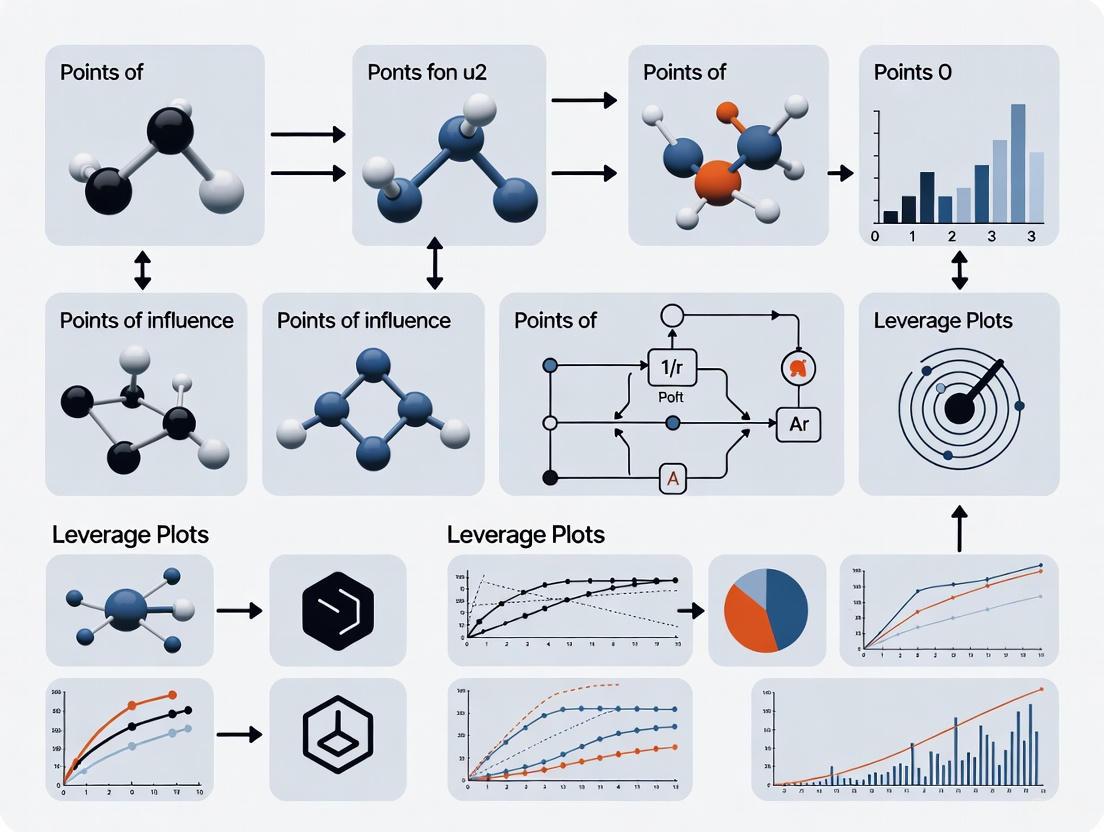
Leverage Plots: A Practical Guide for Identifying Influential Points in Biomedical Research
This guide provides researchers, scientists, and drug development professionals with a comprehensive framework for using leverage plots to detect influential observations in regression analysis.
Leverage Plots: A Practical Guide for Identifying Influential Points in Biomedical Research
Abstract
This guide provides researchers, scientists, and drug development professionals with a comprehensive framework for using leverage plots to detect influential observations in regression analysis. It covers foundational concepts distinguishing outliers, leverage, and influence, offers step-by-step methodologies for creating and interpreting diagnostic plots in statistical software, and presents troubleshooting protocols for addressing high-leverage points. The article also explores advanced validation techniques and compares leverage plots with other diagnostic measures, emphasizing their critical role in ensuring model robustness and data integrity for regulatory compliance and high-impact publications.
Understanding Leverage, Outliers, and Influence in Regression Diagnostics
FAQs on Unusual Observations in Linear Regression
Q1: What is the fundamental distinction between an outlier, a leverage point, and an influential observation?
An outlier is a data point whose response (y-value) does not follow the general trend of the rest of the data [1]. Its dependent variable value is unusual given its predictor values.
A data point has high leverage if it has an extreme or "unusual" predictor (x-value) [1]. In multiple regression, this can mean a value that is particularly high or low for one or more predictors, or an unusual combination of predictor values [1]. A leverage point can follow the regression trend and thus may not be an outlier in the y-direction [2].
An influential point is one that unduly influences any part of the regression analysis, such as the estimated slope coefficients, predicted responses, or hypothesis test results [1]. Its removal from the dataset would cause a substantial change in the fitted model [2]. Influential points are often both outliers and high-leverage points [1].
Q2: How can I statistically test for these unusual points in my dataset?
Diagnostic tests help identify different types of unusual observations [2].
- y-Outlier: Check the residual (RESI), standardized residual (SRES), or studentized deleted residual (TRES). A data point is generally considered an outlier if the absolute value of any of these is high compared to others [2].
- x-Outlier (Leverage): Calculate the diagonal elements of the hat matrix (HI or leverage). The sum of all HI values equals p (the number of parameters plus the intercept). A common rule is that any HI value exceeding
2*p/n(twice the average leverage) indicates a high-leverage point [2]. - Influential Point: Use DFIT or Cook's distance. For small to medium datasets, an absolute DFIT value greater than 1 suggests influence [2]. For Cook's distance, a larger value indicates greater potential influence. The associated p-value from an F-distribution can quantify this: a probability over 50% indicates a major influence, 20-50% a moderate to high influence, and 10-20% a very small influence [2].
Q3: A high-leverage point is not necessarily an influential point. Can you explain why?
Yes, a high-leverage point is not automatically influential [1]. A point with an extreme x-value has the potential to exert strong influence on the regression line. However, if its observed y-value is consistent with the trend predicted by the other data points (i.e., it sits on or near the regression line formed by the other points), then including it will not significantly alter the slope or intercept [1]. In this case, it is a non-influential high-leverage point. Its main effect might be to artificially inflate the R-squared value and the statistical significance of the relationship, making the model appear stronger than it actually is for the bulk of the data [2].
Q4: What is the single most critical check for an observation that is both an outlier and has high leverage?
An observation that is both an outlier (unusual y) and has high leverage (unusual x) has the highest potential to be influential [1]. The most critical check is to assess its Cook's Distance or DFITs to statistically confirm its influence on the entire regression model [2]. You should refit the regression model with and without this point and compare key outputs like the estimated slope, R-squared, and p-values for a comprehensive view of its impact [1].
Troubleshooting Guide: Diagnosing Unusual Observations
| Symptom | Potential Cause | Diagnostic Check | Next Steps / Resolution |
|---|---|---|---|
| A dramatic change in the slope coefficient when a single point is added/removed. | An influential point that is likely both an outlier and has high leverage [1]. | 1. Check Cook's Distance (large value) [2].2. Check Leverage (HI > 2p/n) [2].3. Check Standardized Residual (absolute value > 2 or 3). | Investigate the data point for measurement or data entry error. Report results with and without the point if its validity is uncertain. |
| A very high R-squared value, but the model predictions for most data seem poor. | One or more high-leverage points are artificially strengthening the apparent relationship [2]. | Examine a scatter plot for points isolated in the x-direction. Calculate leverage statistics (HI) [2]. | Consider whether the leverage point is within the relevant scope of your research question. Collect more data in the gap to reduce the point's undue influence. |
| The residual plot shows one point with a very large deviation from zero. | A y-outlier [1]. | Check the residual (RESI) and studentized deleted residual (TRES) for that observation [2]. | Verify the data source and process that generated the point. If it is a valid but extreme value, consider robust regression techniques. |
| The model meets all statistical significance criteria, but a single point is responsible for this conclusion. | An influential point that drives the model's significance [1]. | Check if the point is influential using DFITs. Check if the model remains significant without the point. | Transparency is key. Acknowledge the point's role in the analysis. The model may not be generalizable if it relies on a single observation. |
Quantitative Diagnostics Table
The following table summarizes key statistical measures used to identify unusual observations. These values are typically calculated using statistical software.
| Diagnostic Measure | What it Identifies | Common Interpretation Threshold | Statistical Test / Calculation |
|---|---|---|---|
| Standardized Residual (SRES) | y-Outliers | Absolute value > 2 or 3 suggests a potential outlier [2]. | Residual / Standard Error of Residuals |
| Leverage (HI) | x-Outliers / High-Leverage Points | HI > 2*p/n (where p = # of parameters + intercept, n = sample size) [2]. |
Diagonal element of the Hat matrix. |
| Cook's Distance (D) | Influential Points | D > 1, or a significantly larger D value than other points; or a p-value > 50% from F-distribution indicates major influence [2]. | Complex function of leverage and residual. Measures the change in all fitted values when the i-th point is omitted. |
| DFFITS | Influential Points on Fitted Value | Absolute value > 1 for small/medium datasets [2]. | Standardized difference between the fitted value with and without the i-th observation. |
Experimental Protocol: Identifying Influential Points with Leverage Plots
Objective: To systematically identify and evaluate the impact of outliers, high-leverage points, and influential observations in a linear regression analysis.
1. Data Preparation and Initial Model Fitting
- Collect your dataset and specify your linear regression model.
- Using statistical software (e.g., R, Python, Minitab), fit the initial regression model and obtain the results.
2. Calculation of Diagnostic Statistics
- For every observation in your dataset, calculate and store the following diagnostic statistics:
- Predicted Values (y-hat)
- Residuals (RESI)
- Standardized Residuals (SRES) or Studentized Deleted Residuals (TRES)
- Leverage values (HI) from the hat matrix.
- Cook's Distance
- DFFITS (if available in your software).
3. Graphical Analysis
- Create a residuals vs. fitted values plot to visually check for outliers (points with large vertical deviations from zero) and non-constant variance.
- Create a leverage plot (e.g., studentized residuals vs. leverage) to simultaneously assess outliers and high-leverage points.
- Create an index plot of Cook's Distance to quickly identify the most influential observations.
4. Statistical Threshold Testing
- Apply the interpretation thresholds from the Quantitative Diagnostics Table above:
5. Influence Assessment and Reporting
- Refit the regression model after excluding the flagged influential points.
- Compare the key model parameters (slope, intercept, R-squared, p-values) between the original and the new model.
- Document the changes. In your thesis or report, clearly state the diagnostic process undertaken and the impact of any unusual observations on your final conclusions.
Research Reagent Solutions: Key Statistical Diagnostics
| Item / Software | Function in Analysis |
|---|---|
| Statistical Software (e.g., R, Python with statsmodels, Minitab) | The primary platform for fitting regression models and computing all diagnostic statistics (residuals, leverage, Cook's D) [2]. |
| Hat Matrix (H) | A crucial mathematical construct whose diagonal elements (HI) are the direct measure of an observation's leverage on its own predicted value [2]. |
| Cook's Distance | A single metric that aggregates the overall influence of a single data point on all regression coefficients, used to flag points that disproportionately affect the model [2]. |
| Standardized & Studentized Residuals | Residuals that have been scaled by their standard error, making it easier to identify outliers in the y-direction by providing a common scale for comparison [2]. |
Visualizing the Concepts: A Diagnostic Workflow
The following diagram illustrates the logical process for diagnosing different types of unusual observations in a regression dataset.
Frequently Asked Questions
1. What is the fundamental difference between an outlier and a high leverage point? An outlier is a data point whose response (y-value) does not follow the general trend of the rest of the data, resulting in a large residual [1] [3]. A high leverage point is one that has "extreme" predictor (x-value) values, which may be unusually high, low, or an unusual combination of predictor values in multiple regression [1] [3] [4]. The key difference is that an outlier is unusual in the vertical (y) direction, while a high leverage point is unusual in the horizontal (x) direction.
2. Can a single data point be both an outlier and have high leverage? Yes. A data point that has both an extreme x-value and does not follow the general trend of the data (large residual) is considered both an outlier and a high leverage point [5]. Such a point has a high potential to be influential.
3. What is an influential point, and how does it relate to outliers and leverage? An influential point is a data point that unduly influences any part of a regression analysis if removed, such as the predicted responses, estimated slope coefficients, or hypothesis test results [1] [3]. While outliers and high leverage points have the potential to be influential, they are not always so. An influential point is one that, when removed, significantly changes the regression model [5]. An outlier that is also a high leverage point is the most likely to be influential [1] [5].
4. Why is it important to distinguish between these types of unusual points? Identifying and correctly classifying these points is crucial because they can skew the results of a regression analysis in different ways. Understanding whether a point is an outlier, has high leverage, or is influential helps a researcher decide the most appropriate course of action, whether it's investigating the data point for errors, using robust regression techniques, or reporting the findings with and without the point [1] [3].
5. What are some robust regression techniques to use when my data has outliers? Several robust regression techniques are less sensitive to outliers, including [6] [7]:
- Huber Regression: Uses a loss function that is less sensitive to outliers by combining squared loss for small residuals and absolute loss for large residuals.
- RANSAC Regression (RANdom SAmple Consensus): An iterative algorithm that fits a model to random subsets of data, identifying inliers and outliers.
- Theil-Sen Regression: Calculates the slope as the median of all slopes between pairs of points, making it robust to outliers.
Troubleshooting Guides
Guide 1: Diagnosing Unusual Observations in Your Regression
Use the following workflow to systematically identify and classify unusual points in your dataset. This process is integral to validating the assumptions of your leverage plots research.
Diagram 1: A diagnostic workflow for classifying unusual observations.
Experimental Protocol & Diagnostic Measures
After following the workflow, use these specific statistical measures to diagnose each type of point. The following table summarizes the key diagnostic statistics and their interpretation, which should be calculated as part of your experimental protocol.
Table 1: Diagnostic Measures for Unusual Observations [4] [8] [2]
| Point Type | Primary Diagnostic Measure | Interpretation & Common Threshold | Secondary Measures | ||
|---|---|---|---|---|---|
| High Leverage | Leverage ($h_{ii}$) [4] | $h_{ii} > 2p/n$ indicates high leverage, where $p$ is the number of parameters (including intercept) and $n$ is the number of observations [4] [2]. | Partial Leverage [4] | ||
| Outlier | Standardized Residual ($r_i$) [8] | $ | r_i | > 2$ or $3$ suggests an outlier. $ri = \frac{ei}{\sqrt{MSE(1-h_{ii})}$ [8]. | Studentized Residuals, Deleted Residuals [2] |
| Influential | Cook's Distance ($D$) [2] | Compare $D$ to an F-distribution with $p$ and $n-p$ degrees of freedom. A probability > 50% indicates major influence [2]. | DFITS [2] |
Protocol Steps:
- Fit the Model: Fit your initial regression model to the full dataset.
- Calculate Leverage: Compute the leverage statistic ($h_{ii}$) for each observation. This is typically the diagonal element of the hat matrix [4].
- Flag High Leverage: Identify points where $h_{ii} > 2p/n$ [4] [2].
- Calculate Residuals: Compute the standardized residuals for each observation [8].
- Flag Outliers: Identify points where the absolute value of the standardized residual exceeds your chosen threshold (e.g., 2 or 3) [8].
- Test for Influence: For points flagged as high leverage, outliers, or both, calculate Cook's Distance. A point is considered influential if its exclusion causes a substantial change in the regression coefficients [1] [2]. This can be tested by visually comparing regression lines with and without the point, or by using the statistical thresholds for Cook's D [2].
Guide 2: Addressing Influential Points in Analysis
Once you have diagnosed unusual points, follow this guide to address them.
Step 1: Investigate the Point
- Check for Data Errors: Verify the data was entered and processed correctly. Simple transcription errors are a common cause.
- Understand Context: Determine if the point represents a rare but valid biological event. In drug development, this could indicate a unique responder or a specific experimental condition.
Step 2: Choose an Analytical Strategy The appropriate strategy depends on whether the point is truly an error and the goals of your analysis.
Table 2: Strategies for Handling Unusual Points [6] [7] [9]
| Scenario | Recommended Strategy | Rationale & Implementation |
|---|---|---|
| Point is a data error | Remove the point | The point does not represent the underlying phenomenon and will bias the results. Re-fit the model without the point. |
| Point is valid but influential | Report analyses both with and without the point. | Provides transparency and allows readers to see the impact of a single observation on the conclusions. |
| Model must be robust to outliers | Use Robust Regression (e.g., Huber, RANSAC, Theil-Sen) [6] [7] | These algorithms are designed to be less sensitive to outliers, reducing their influence without manually removing them. |
| The point is a valid high leverage point | Retain the point and acknowledge it extends the model's scope. | A high leverage point that is not an outlier provides important information about the relationship at extreme X-values and improves the estimate of the slope [1]. |
Step 3: Document and Report Always document any unusual points found and the actions taken. In your thesis and publications, report:
- The number and nature of unusual points.
- Diagnostic statistics (e.g., leverage, Cook's D).
- A comparison of results with and without influential points.
- The final chosen model and the rationale for the choice.
The Scientist's Toolkit
Table 3: Key Research Reagent Solutions for Robust Analysis
| Tool / Solution | Function in Analysis |
|---|---|
| Statistical Software (R, Python) | Platform for calculating diagnostic statistics (leverage, residuals, Cook's D) and fitting robust regression models [6] [7]. |
| Leverage (Hat) Matrix | The mathematical matrix whose diagonal elements ($h_{ii}$) are the direct measure of leverage for each observation [4]. |
| Huber Loss Function | The core function used in Huber Regression, which combines squared and absolute loss to reduce the weight given to outliers during model fitting [6] [7]. |
| RANSAC Algorithm | A non-deterministic, iterative algorithm for separating inliers from outliers in a dataset, effective for datasets with a large proportion of outliers [6] [7]. |
| Cook's Distance Metric | A statistical measure that aggregates the influence of a single data point on all fitted values, used to flag points for further investigation [2]. |
FAQs and Troubleshooting Guide
This guide provides solutions to common issues researchers face when using leverage plots to identify influential points in statistical models, particularly in drug development.
Q1: What does a "Leverage of 1.0" mean in my plot, and is it a problem?
A leverage value of 1.0 indicates a point that has the maximum possible influence on the model's fit. This is often a sign of a perfect fit for that single point, which can distort the overall model.
- Troubleshooting Steps:
- Investigate the Point: Check your raw data for this observation. Look for data entry errors, measurement malfunctions, or a unique biological outlier that doesn't belong to the population you are modeling.
- Run Diagnostics: Fit your model with and without this high-leverage point. Compare the model coefficients, R-squared, and p-values. If they change dramatically, the point is highly influential.
- Document and Decide: Based on your investigation, decide if the point is a valid but extreme value (which you may keep, but note in your report) or an error (which you should correct or remove). Never remove a point solely for statistical reasons without a scientific justification.
Q2: My leverage plot shows a point with high leverage but a small residual. Should I be concerned?
A point with high leverage but a small residual (close to the regression line) is not necessarily a problem. It means this point is an extreme value in the predictor space, but the model's prediction for it is still accurate. It can strengthen the model's fit rather than distort it.
- Action: Monitor this point, but it typically does not require removal. Its primary effect is to reduce the standard errors of your coefficient estimates, increasing the precision of your model.
Q3: How do I handle a cluster of points with high leverage?
A cluster of high-leverage points suggests a subgroup within your data. This is common in drug development, for example, when data comes from different experimental batches or patient subpopulations.
- Troubleshooting Steps:
- Validate the Subgroup: Determine if the cluster represents a scientifically relevant category (e.g., responders vs. non-responders, a specific dosage group).
- Consider Model Expansion: Your current model might be oversimplified. You may need to include an additional factor or interaction term in your model to account for this subgroup.
- Check for Confounding: Ensure that the cluster is not an artifact of an uncontrolled experimental variable.
Q4: What is the difference between leverage and influence?
While often related, leverage and influence are distinct concepts, as shown in the table below.
- Table: Leverage vs. Influence
Feature Leverage Influence (e.g., Cook's Distance) Definition A point's potential to influence the model, based on its position in the predictor space. A point's actual impact on the model's coefficients and predictions. Depends On Only the values of the independent variables (X). The values of both independent (X) and dependent (Y) variables. What to Look For Points that are distant from the mean of the predictors. Points that have high leverage and a large residual (don't fit the trend). Primary Metric Hat values (diagonals of the hat matrix). Cook's Distance, DFFITS, DFBETAS.
The following table summarizes key thresholds for common diagnostic statistics used alongside leverage plots. These are rules of thumb; context is critical.
- Table: Key Diagnostic Statistics and Thresholds
Diagnostic Statistic Calculation Common Threshold for Concern Interpretation Leverage (h~ii~) Diagonal of hat matrix > 2p/n Potential for high influence. Cook's Distance (D) Combined measure of leverage and residual > 4/n Significantly influences model coefficients. Studentized Residual Residual scaled by its standard deviation > 2 A potential outlier in the Y-direction. DFFITS Change in predicted value when point is omitted > 2√(p/n) Influences its own fitted value.
Where *n is the number of observations and p is the number of model parameters.*
Experimental Protocol: Identifying Influential Points with Leverage Plots
Objective: To detect and diagnose data points that have a strong potential to influence a linear regression model, ensuring the model's robustness and validity.
Materials:
- Statistical software (e.g., R, Python with
statsmodels/scikit-learn, SAS, JMP). - Dataset with continuous outcome and predictor variables.
Methodology:
Model Fitting:
- Fit your initial linear regression model to the data:
Y ~ X1 + X2 + ... + Xp.
- Fit your initial linear regression model to the data:
Calculation of Diagnostic Statistics:
- Extract the following statistics for every observation in the dataset:
- Leverage (Hat Values): Measures the potential influence.
- Residuals: The difference between observed and predicted values.
- Cook's Distance: A combined measure of a point's leverage and the size of its residual.
- Extract the following statistics for every observation in the dataset:
Visualization with Leverage Plots:
- Create a Residuals vs. Leverage plot.
- On this plot, the size of each point can be mapped to its Cook's Distance, creating a bubble plot. This allows for the simultaneous assessment of all three key diagnostics.
Interpretation and Diagnosis:
- Identify points that fall above the leverage threshold.
- Among high-leverage points, focus on those that also have large residuals (far from zero on the y-axis) and/or a large bubble size (high Cook's Distance). These are your most influential points.
Sensitivity Analysis:
- Refit the regression model after removing the flagged influential points.
- Systematically compare the key outputs (coefficients, standard errors, R-squared) of the original and new model to quantify the influence.
The workflow for this protocol is outlined in the diagram below.
The Scientist's Toolkit: Research Reagent Solutions
- Table: Essential Materials for Statistical Analysis of Influential Points
Item Function/Brief Explanation R Statistical Software Open-source environment for statistical computing and graphics. Essential for advanced regression diagnostics. statsmodelsLibrary (Python)A Python module that provides classes and functions for estimating many different statistical models and conducting statistical tests and explorations. Diagnostic Plots Package (e.g., carin R,statsmodels.graphicsin Python)Specialized software libraries designed specifically for creating regression diagnostic plots, including leverage plots and plots of Cook's Distance. Cook's Distance Metric A quantitative measure that combines leverage and residual information to estimate a point's overall influence on the regression model. Data Visualization Library (e.g., ggplot2in R,matplotlib/seabornin Python)Libraries used to create custom, publication-quality plots for visualizing data distributions, model fits, and diagnostic statistics.
Frequently Asked Questions (FAQs)
1. What is the Hat Matrix in linear regression? The Hat Matrix, denoted as H, is a fundamental mathematical construct in linear regression that projects the vector of observed response values onto the space spanned by the model's predictor variables [10] [11]. It is defined by the formula ( H = X(X^{T}X)^{-1}X^{T} ), where ( X ) is the data matrix of predictor variables [4] [12]. This matrix puts the "hat" on the observed response vector ( y ) to generate the predicted values ( \hat{y} ) via the equation ( \hat{y} = Hy ) [12] [13]. Its diagonal elements, known as leverage scores, are critical for diagnosing potential influential points in regression analysis.
2. What is a leverage score and what does it measure? A leverage score is the ( i )-th diagonal element, ( h_{ii} ), of the Hat Matrix [10] [4]. It quantifies the potential influence of the ( i )-th observation on its own predicted value, based solely on its position in the predictor variable space [12] [13]. A high leverage score indicates that an observation has an unusual combination of predictor values compared to the rest of the data set, making it distant from the center of the other observations in the ( X )-space [10] [12].
3. What is the difference between a high-leverage point and an influential point? This is a critical distinction. A high-leverage point has an unusual or extreme value in its predictor variables (a high ( h{ii} )) [2] [14]. However, if its response value ( yi ) follows the general trend of the other data, its high leverage may not unduly affect the regression model. An influential point, on the other hand, is one that actually does exert a disproportionate effect on the regression results—such as the estimated coefficients, ( R^2 ), or p-values—when it is included or excluded from the analysis [2] [14] [13]. All influential points are high-leverage, but not all high-leverage points are influential.
4. How can I calculate leverage scores using statistical software?
After fitting a linear regression model (e.g., using fitlm or stepwiselm in MATLAB), the leverage values can be directly accessed as a diagnostic property of the fitted model object. For a model named mdl, the command would be mdl.Diagnostics.Leverage [10]. In many software environments, you can also use specialized diagnostic plotting functions, such as plotDiagnostics(mdl), to visually inspect the leverage values [10].
5. What are the key mathematical properties of leverage scores? The leverage scores, ( h_{ii} ), possess several key properties that are useful for diagnostics [4] [12] [13]:
- Bounded Range: Each ( h_{ii} ) is a value between 0 and 1, inclusive.
- Sum Equals Parameters: The sum of all ( h_{ii} ) equals ( p ), the number of parameters in the regression model (including the intercept). This implies that the mean leverage is always ( \bar{h} = p/n ).
- Distance Measure: ( h_{ii} ) is a standardized measure of the distance between the ( i )-th observation's predictor values and the mean predictor values of all ( n ) observations.
Troubleshooting Guides: Identifying and Handling High Leverage Points
Guide 1: How to Diagnose High Leverage Observations
Problem: A researcher suspects that a few observations in their dataset, due to their extreme values in predictor variables, might have an undue potential to influence the regression model.
Solution Protocol: Follow this step-by-step guide to calculate, visualize, and interpret leverage scores.
Step 1: Compute Leverage Scores Fit your linear regression model and extract the leverage values. These are the diagonal elements of the hat matrix ( H ) [10] [4].
Step 2: Visual Inspection Create a leverage index plot—a simple scatter plot with the observation index ( i ) on the x-axis and the leverage value ( h_{ii} ) on the y-axis [10]. This helps quickly spot observations with unusually high bars.
Step 3: Apply Decision Rules Use established statistical rules of thumb to flag high-leverage points. A common practice is to compare each leverage value to a multiple of the average leverage, ( \bar{h} = p/n ) [12] [13].
Table 1: Common Thresholds for Identifying High Leverage Points
| Threshold Rule | Formula | Interpretation |
|---|---|---|
| Common Cut-off [12] [13] | ( h_{ii} > 3 \times (p/n) ) | Observations exceeding this value are often flagged as "Unusual X" and warrant investigation. |
| Refined Cut-off [12] [13] | ( h_{ii} > 2 \times (p/n) ) | A more sensitive threshold. Often used to identify points that are both high-leverage and isolated from other data. |
Step 4: Contextual Analysis Examine the flagged observations in the context of your research. Are these values plausible, or could they be data entry errors? Do they belong to a known but rare sub-population? This step requires domain expertise [2].
Guide 2: How to Determine if a High-Leverage Point is Influential
Problem: A high-leverage point has been identified. The researcher needs to determine if this point is truly influential on the regression results.
Solution Protocol: Use deletion diagnostics to quantify the actual impact of removing the suspect observation.
Step 1: Calculate Influence Measures For each observation ( i ) flagged as high-leverage, compute one or more of the following influence measures. These metrics estimate the change in regression outputs when the ( i )-th observation is omitted.
Table 2: Key Influence Diagnostics for Regression Analysis
| Diagnostic Measure | What it Quantifies | Common Threshold |
|---|---|---|
| DFBETA / DFBETAS [15] | The change in each regression coefficient ( \beta_j ) when the ( i )-th observation is removed. DFBETAS is the standardized version. | ( \mid \text{DFBETAS} \mid > \frac{2}{\sqrt{n}} ) |
| Cook's Distance [2] | A combined measure of the influence of observation ( i ) on all fitted values. | A common rule is to flag points where Cook's D is greater than the 50th percentile of an F-distribution with ( p ) and ( n-p ) degrees of freedom [2]. |
| DFFITS [2] | The change in the predicted value for observation ( i ) when it is removed from the fitting process. | ( \mid \text{DFFITS} \mid > 1 ) (for small/medium datasets) |
Step 2: Fit Models with and Without the Point As a direct validation, refit the regression model after excluding the high-leverage observation(s). Compare key outputs like coefficient estimates, R-squared, and p-values between the two models [14]. Substantial changes indicate influence.
Step 3: Decision and Reporting
- If the point is not influential, it may be safe to retain it, but its existence should be noted as it can make the model's predictions less precise in its region of the predictor space [2].
- If the point is influential, investigate its origin. If it stems from a data error, correct it. If it is a valid but unusual observation, report your model results both with and without the point to ensure transparency about the fragility of your findings [15] [13].
Visualizing the Analytical Workflow
The following diagram illustrates the logical process for diagnosing and handling unusual observations in a regression analysis.
Table 3: Key Research Reagent Solutions for Leverage Analysis
| Tool / Resource | Function in Analysis | Implementation Example |
|---|---|---|
| Hat Matrix (H) | The core mathematical object whose diagonal elements are the leverage scores. It projects observed responses into predicted values [12] [11]. | ( H = X(X^{T}X)^{-1}X^{T} ) |
| Leverage Vector | A vector containing all diagonal elements ( h_{ii} ) of H. It is the primary input for identifying observations with extreme predictor values [10]. | Accessed via mdl.Diagnostics.Leverage in MATLAB [10]. |
| Index Plot | A simple visualization to quickly scan for observations with unusually high leverage scores compared to others [10]. | Use plotDiagnostics(mdl, 'Leverage') or equivalent in your software. |
| DFBETAS | Standardized values that measure the effect of deleting the ( i )-th observation on each regression coefficient ( \beta_j ). Crucial for pinpointing which parameters are affected [15]. | In R, use dfbetas(model). A common threshold is ( 2/\sqrt{n} ). |
| Cook's Distance | A single, overall measure of the influence of an observation on the entire set of regression coefficients and predictions [2]. | Available in most statistical software regression diagnostics. Flag points with a large Cook's D relative to others. |
Frequently Asked Questions
What is an influential point in regression analysis? An influential point is an observation that, individually, exerts a large effect on a regression model's results—the parameter estimates (β̂) and, consequently, the model's predictions. Influential points are not necessarily problematic, but they warrant follow-up investigation as they can signal data-entry errors or observations that are unrepresentative of the population of interest [15].
How can a single data point significantly change my regression results? A single point can be influential if it has high leverage (an unusual value for a predictor variable) and high outlyingness (an unusual value for the response variable). Such a point can "drag" the entire regression line toward itself. For example, a single misrecorded data point can change a slope estimate from positive to negative, fundamentally altering the interpretation of the relationship between variables [15].
What is the difference between DFBETA and DFBETAS? DFBETA and DFBETAS are metrics used to quantify a point's influence on a specific regression coefficient.
- DFBETA is the raw change in a regression coefficient when the ith observation is removed:
DFBETA_ij = β̂_j - β̂_(i)j[15]. - DFBETAS is a standardized version, calculated by dividing the DFBETA by the standard error of the coefficient estimate. This makes DFBETAS values comparable across different models and variables, as they are free from the scale of the variables [15].
How do I interpret an Effect Leverage Plot? An Effect Leverage Plot (also known as a partial regression plot) visualizes the influence of individual points on the test for a specific term in the model [16] [17].
- The Fitted Line (Red): Shows the model with the term included. Its slope is the coefficient estimate for that term.
- The Horizontal Line (Blue): Represents the model without the term (the hypothesis that the coefficient is zero) [16].
- Point Positions: Points that are far from the horizontal line exert more influence on the hypothesis test. A point far from the bulk of the data can have a large influence on the parameter estimate [17].
- Confidence Curves (Shaded Red): If these curves cross the horizontal blue line, the effect is statistically significant. If the blue line lies entirely within the confidence region, the effect is not significant [16].
Is there a definitive cut-off for identifying an influential point?
While no perfect cutoff exists, a common and size-adjusted threshold for |DFBETAS| is 2/√n, where n is the sample size. This threshold helps expose a similar proportion of potentially influential observations regardless of the sample size [15].
The table below shows how this threshold changes with sample size:
| Sample Size (n) | Threshold for |DFBETAS| |
|---|---|
| 50 | ~0.283 |
| 100 | 0.200 |
| 500 | ~0.089 |
| 1000 | ~0.063 |
Troubleshooting Guides
Issue: Suspecting that influential points are distorting regression coefficients
Investigation Protocol:
- Calculate Influence Statistics: Use statistical software to compute DFBETA or DFBETAS for each observation and each coefficient. Most software packages have built-in functions for this (e.g.,
dfbeta()anddfbetas()in R) [15]. - Visualize with Effect Leverage Plots: Generate a leverage plot for each predictor variable in your model. These plots will help you see which points might be exerting influence on the test for that specific variable [16].
- Compare to Threshold: Compare the absolute DFBETAS values to the
2/√nthreshold. Any observation with a |DFBETAS| value exceeding this threshold for any coefficient should be flagged for further investigation [15]. - Inspect Flagged Points: Manually examine the raw data for the flagged observations. Check for potential data entry errors, measurement errors, or unique characteristics that might make the observation fundamentally different from the rest of your dataset.
Resolution Actions:
- If a data error is found: Correct the error if possible, then re-run the analysis.
- If the point is valid but influential: It is critical to report your model results both with and without the highly influential points. This transparency shows the fragility of your model's results and allows readers to assess the impact of these points on your conclusions [15].
- Consider model re-specification: In some cases, the presence of influential points may indicate that your model is misspecified (e.g., missing a key variable or requiring a different functional form).
Issue: Diagnosing multicollinearity from a Leverage Plot
Symptoms: In an Effect Leverage Plot, the points appear to collapse toward a vertical line or cluster very tightly toward the middle of the plot. This indicates that the predictor variable is highly correlated with other predictors already in the model [16] [17].
Interpretation: This clustering shows that the variable adds little new information, making the slope of the fitted line unstable. The standard error for the coefficient will be inflated, and the parameter estimate can be unreliable [16].
Next Steps: Investigate variance inflation factors (VIFs) for a quantitative measure of multicollinearity. You may need to remove variables, combine them, or use regularization techniques like ridge regression.
Experimental Protocols & Methodologies
Protocol: Calculating and Interpreting DFBETAS
Objective: To quantitatively assess the influence of each observation on each estimated regression coefficient.
Procedure:
- Fit the Full Model: Regress the response variable Y on all predictor variables (X₁, X₂, ..., Xₚ) using all
nobservations. Obtain the coefficient estimates β̂_j for each predictor. - Fit the Reduced Models: For each observation
i(from 1 ton), fit the same regression model but with the ith observation omitted. Obtain the new coefficient estimates β̂_(i)j. - Compute DFBETA: For each observation
iand each coefficientj, calculate:DFBETA_ij = β̂_j - β̂_(i)j[15] - Compute DFBETAS: Standardize the DFBETA values. For linear regression, the formula is:
DFBETAS_ij = (β̂_j - β̂_(i)j) / SE(β̂_j)where the standard error is calculated using the mean squared error from the regression with the ith observation deleted [15]. - Identify Influential Points: Flag any observation where |DFBETAS_ij| >
2/√nfor any variablej[15].
Protocol: Constructing and Interpreting an Effect Leverage Plot
Objective: To visually assess the influence of individual points on the significance test for a specific model effect and to spot multicollinearity.
Construction Workflow for a Continuous Predictor X:
Interpretation Guide:
- Significance: The effect of variable X is statistically significant if the confidence curves for the fitted red line cross the horizontal blue line (which represents the hypothesis that the coefficient for X is zero) [16].
- Influence: Points that are horizontally distant from the center of the plot have higher leverage and exert more influence on the test for X. A high-leverage point that is also far from the fitted line can have a large influence on the parameter estimate itself [16] [17].
- Multicollinearity: If the points collapse toward a vertical line, it indicates that X is highly collinear with other predictors in the model [17].
The Scientist's Toolkit: Research Reagent Solutions
Essential materials and statistical measures for conducting influence analysis in regression modeling.
| Item / Solution | Function in Analysis |
|---|---|
| DFBETA | Measures the raw change in a coefficient when an observation is omitted; used for direct assessment of influence on parameter estimates [15]. |
| DFBETAS | The standardized version of DFBETA; allows for comparison across different coefficients and models via a common, scale-free threshold [15]. |
| Effect Leverage Plot | A diagnostic plot that visualizes the unique effect of a predictor and the influence of each data point on its significance test [16] [17]. |
| Size-Adjusted Threshold (2/√n) | Provides a sample-size-dependent cut-off for DFBETAS to identify potentially influential points in a consistent manner [15]. |
| Statistical Software (R, JMP, etc.) | Platforms with built-in functions (e.g., dfbetas()) and visualization tools (e.g., Effect Leverage Plots) to efficiently compute diagnostics and create plots [15] [16]. |
Creating and Interpreting Leverage Plots: A Step-by-Step Protocol
Table of Contents
- Introduction to Leverage Plots
- Implementation in SAS
- Implementation in R
- Implementation in Python
- Troubleshooting FAQs
- Research Reagent Solutions
Leverage plots are powerful diagnostic tools in regression analysis for identifying influential observations. Within the context of identifying influential points, it is crucial to distinguish between different types of "unusual" data: outliers (points with large residuals, extreme y-values), high-leverage points (points with extreme x-values), and influential points (points that significantly alter the regression model when removed) [18] [5]. An influential observation is often one that possesses both high leverage and a large residual [18] [19].
The following diagram illustrates the logical relationship between these concepts and the role of leverage plots in the diagnostic process.
Implementation in SAS
SAS provides a direct method for generating partial regression leverage plots through PROC REG, which visualizes the relationship between a specific predictor and the response variable after accounting for all other predictors [20].
Detailed Methodology:
- Data Preparation: Use a
DATA STEPto load and prepare your dataset. Ensure variables are appropriately labeled [20]. - Enable Graphics: Use
ods graphics on;to allow the production of graphical output [20]. - Run Regression Model: In
PROC REG, use thePLOTS(ONLY)=(PARTIAL)and thePARTIALoption in theMODELstatement to generate only the partial regression leverage plots [20]. - Interpretation: In each plot, the slope of the fitted line corresponds to the coefficient estimate for that variable in the full model. A near-horizontal line suggests the predictor may not be statistically significant [20].
Example Code:
Implementation in R
In R, you can calculate leverage statistics and create diagnostic plots using base R functions. The process involves fitting a model and then extracting leverage values from the model object [21].
Detailed Methodology:
- Fit Regression Model: Use the
lm()function to fit a linear regression model. - Calculate Leverage: The
hatvalues()function applied to the model object returns the leverage statistics for each observation [21]. - Visualize Leverage: Use the
plot()function withtype = 'h'to create a leverage index plot, which shows each observation's leverage value [21]. Observations with leverage greater than2*mean(leverage)or3*mean(leverage)are often flagged for further investigation [19]. - Comprehensive Diagnostics: The
plot(model)command automatically generates a series of four diagnostic plots, including a "Residuals vs Leverage" plot which is key for spotting influential points [22].
Example Code:
Implementation in Python
Python's statsmodels library offers a comprehensive suite for statistical modeling, including the creation of various regression diagnostic plots similar to R [22].
Detailed Methodology:
- Import Libraries: Key libraries are
statsmodels.api(for OLS regression) andmatplotlib.pyplot(for plotting) [22]. - Fit OLS Regression: Use
statsmodels.formula.api(orstatsmodels.api) to specify and fit an Ordinary Least Squares (OLS) model [22]. - Extract Diagnostic Variables: From the fitted model, extract components like residuals, fitted values, standardized residuals, and leverage values using
results.get_influence().hat_matrix_diag[22]. - Create Diagnostic Plots: Use
matplotlibto create a grid of plots, including a "Residuals vs Leverage" plot. Thestatsmodels.graphics.influence_plot()creates a specialized plot that combines information about leverage and influence (Cook's distance) [22].
Example Code:
Troubleshooting FAQs
FAQ 1: What is the difference between an outlier, a high-leverage point, and an influential point? These terms describe different types of "unusual" data in a regression context. An outlier has an extreme value for the response variable (Y), leading to a large residual as it does not follow the general trend of the data [5]. A high-leverage point has an extreme value for one or more predictor variables (X) [5]. An influential point is one that, if removed, substantially changes the estimate of the regression coefficients (e.g., the slope or intercept) [5]. An influential point is typically both an outlier and a high-leverage point [18].
FAQ 2: My leverage plot doesn't show a reference line for Cook's distance in Python. How can I add it?
The influence_plot in statsmodels automatically adds Cook's distance as concentric circles. For manual plots, you can calculate Cook's distance using results.get_influence().cooks_distance[0] and then add contour lines to your scatter plot. You would need to calculate the Cook's distance values for a grid of leverage and residual values, which is a non-trivial process. Using the built-in influence_plot is recommended for this purpose [22].
FAQ 3: How do I label specific influential points in my R or Python plot?
In R, after creating the base plot, you can use the text() or points() functions with a logical condition to label points with high leverage or influence. For example, text(leverage, residuals, labels=ifelse(leverage > threshold, row.names(mtcars), ""), pos=4).
In Python, when using matplotlib, you can loop through your data points and use ax.annotate() to add text labels for points that meet your criteria (e.g., high Cook's distance). The influence_plot from statsmodels automatically labels the most influential points [22].
FAQ 4: What are the common thresholds for identifying high-leverage points? There are several rules of thumb:
- A leverage value greater than
2 * (p / n)or3 * (p / n), wherepis the number of predictors (including the intercept) andnis the number of observations, is often considered a high-leverage point [19]. - Huber's guideline suggests that leverage values
pᵢᵢ ≤ 0.2are safe, values0.2 < pᵢᵢ ≤ 0.5are risky, and valuespᵢᵢ > 0.5should be avoided or investigated thoroughly [19]. - Note that leverage values always fall between
1/nand1[21].
Research Reagent Solutions
The table below lists key software and computational "reagents" essential for conducting research on influential points with leverage plots.
| Research Reagent | Function / Purpose | Key Features / Notes |
|---|---|---|
SAS PROC REG [20] |
Fits linear regression models and generates diagnostic plots, including partial regression leverage plots. | The PARTIAL option in the model statement is specific for creating partial leverage plots. Highly reliable in clinical and pharmaceutical research. |
R stats Package [21] |
Core statistical functions for model fitting (lm) and diagnostics (hatvalues, plot.lm). |
Provides fundamental tools for leverage and influence analysis. The base R diagnostic plots are a quick and standard way to assess a model. |
Python statsmodels [22] |
A comprehensive library for estimating and analyzing statistical models. | Its OLS implementation provides detailed summary tables and specialized diagnostic plots (influence_plot), closely mirroring the functionality of R. |
| Cook's Distance [22] [19] | A statistical measure that combines leverage and residual size to quantify an observation's overall influence on the model. | Implemented in both R (cooks.distance) and Python (results.get_influence().cooks_distance[0]). A larger value indicates a more influential point. |
| Hat Values (Leverage) [21] [19] | The diagonal elements of the "hat" matrix. Measure an observation's potential influence based solely on its position in the predictor variable space. | Calculated via hatvalues() in R and get_influence().hat_matrix_diag in Python. It is a key input for identifying high-leverage points. |
Constructing Effect Leverage Plots for Individual Model Terms
Understanding Effect Leverage Plots
An effect leverage plot, also known as a partial regression leverage plot or an added variable plot, is a diagnostic tool that shows the unique, marginal effect of a specific term in your regression model [17]. It answers the question: "What is the effect of adding this particular predictor to a model that already contains all the other predictors?"
The plot visualizes the relationship between the response variable and the predictor of interest, after both have been adjusted for, or "purified" of, the effects of all other predictors in the model [17]. This allows you to see the direct contribution of a single term.
- The Slanted Line: Represents the fitted regression line for the full model with the term included. Its slope is equal to the coefficient estimate for that term in your full model.
- The Horizontal Line: Represents the constrained model without the term. It has a slope of zero for the term in question [17].
- Data Points: These are the partial residuals for the term. The vertical distance from a point to the horizontal line shows the total effect. The vertical distance to the slanted line shows the residual after the term's effect is accounted for.
Points that are far from the horizontal line but close to the slanted line are well-explained by the term. Points that are far from the horizontal line and still distant from the slanted line are outliers for this specific relationship. Points that are distant from the bulk of the data along the x-axis have high leverage on the term's coefficient [17].
The following diagram illustrates the core logical process for creating and interpreting these plots.
Frequently Asked Questions (FAQs)
1. What is the difference between a point with high leverage and an influential point?
While these terms are related, they describe different characteristics of an unusual observation. The table below clarifies the distinctions.
| Feature | Leverage Point | Influential Point | ||
|---|---|---|---|---|
| Definition | A point with an unusual combination of values for the predictor variables (an x-outlier) [2]. | A point that, if removed, causes a substantial change in the regression coefficients, predictions, or other model statistics [15] [2]. | ||
| Primary Cause | Extreme value in one or more independent variables (high x-value) [2]. | A combination of high leverage and an outlying y-value that does not follow the overall trend [15] [2]. | ||
| Impact on Model | Increases the apparent strength of the model (can inflate R-squared) and can make the model overly broad. It has little impact on the coefficient estimates if it follows the overall trend [2]. | Unduly influences the model's outcomes, potentially altering the slope, intercept, p-values, and R-squared, which can lead to misleading conclusions [2]. | ||
| Detection Method | Hat Values (Leverage Statistics): The diagonal elements of the "hat matrix." A common rule of thumb is that a point has high leverage if its hat value exceeds ( \frac{2p}{n} ), where ( p ) is the number of model parameters and ( n ) is the sample size [2]. | DFBETAS: Measures the standardized change in a coefficient when the i-th point is removed. A threshold of ( | DFBETAS | > \frac{2}{\sqrt{n}} ) is often used to flag influence [15]. Cook's Distance: Measures the overall influence of a point on all fitted values. Larger values indicate greater influence [2]. |
2. How do I know if a term is significant based on its effect leverage plot?
If the confidence band around the slanted regression line in the effect leverage plot fully encompasses the horizontal reference line (the model without the term), you can conclude that the term does not contribute significantly to the model. This is visually equivalent to a non-significant F-test for the partial effect of that term [17].
3. My effect leverage plot shows points far from the rest. Should I remove them?
Not necessarily. The first step is to investigate [15]. Check for data entry errors or a valid scientific reason (e.g., a unique patient subgroup) that explains the point's unusual nature. Never remove points simply to improve model fit. Always report the presence of highly influential points and any actions taken, as this is key to research transparency. Consider presenting model results both with and without these points to demonstrate the robustness (or fragility) of your findings [15].
Experimental Protocol: Creating and Analyzing Plots
This protocol provides a step-by-step methodology for constructing effect leverage plots and diagnosing influential points, tailored for research in drug development.
Objective: To visualize the marginal effect of individual predictor variables in a multiple regression model and identify observations that unduly influence the parameter estimates.
Materials & Reagents:
- Statistical Software: R (recommended), SAS, or Python with
statsmodelslibrary. - Computing Environment: Standard desktop computer or server.
- Data: A cleaned dataset containing the continuous response variable (e.g., drug efficacy, IC50 value) and all predictor variables (e.g., dosage, patient biomarkers, chemical descriptors).
Procedure:
- Model Fitting: Fit your full multiple linear regression model containing all terms of interest to the dataset.
- Plot Generation: Use the appropriate function in your statistical software to generate the suite of effect leverage plots (one for each model term).
- In R: Use the
termplotfunction or theavPlotsfunction from thecarpackage.
- In R: Use the
- Visual Inspection: For each plot, examine the position of the slanted line relative to the horizontal line to gauge the term's significance.
- Leverage Diagnosis: Identify points with high leverage—those that lie far from the mean of the partial regressor values (along the x-axis).
- Influence Calculation: Calculate influence statistics. The table below outlines key metrics and their diagnostic thresholds.
| Diagnostic Metric | Formula / Rule of Thumb | Interpretation | R Function | ||
|---|---|---|---|---|---|
| Leverage (Hat Value) | ( h_{ii} > \frac{2p}{n} ) | Flags an observation as an x-outlier with potential to influence the model [2]. | hatvalues(model) |
||
| DFBETAS | ( \left | DFBETAS_{ij} \right | > \frac{2}{\sqrt{n}} ) | Flags an observation as significantly influencing the j-th coefficient estimate [15]. | dfbetas(model) |
| Cook's Distance | Visual inspection; compare distances. A probability >50% based on F-distribution indicates major influence [2]. | Measures the overall influence of an observation on all fitted values [2]. | cooks.distance(model) |
- Follow-up Analysis: For any observation flagged by the above diagnostics, return to the raw data to verify its accuracy and investigate its scientific validity before deciding on its inclusion or exclusion.
The analytical workflow for this protocol, from data preparation to final decision-making, is summarized in the diagram below.
The Scientist's Toolkit: Key Reagents & Solutions
The following table lists the essential "research reagents" — the statistical diagnostics and functions — required for a robust analysis of leverage and influence.
| Research Reagent | Function / Purpose |
|---|---|
| Effect Leverage Plot | Visually isolates the partial effect of a single model term, showing its unique contribution after accounting for all other variables [17]. |
| Hat Values (Leverage Statistics) | Quantifies how unusual an observation's predictor values are, identifying points with the potential to exert influence on the model fit [2]. |
| DFBETAS | A standardized measure of how much a specific regression coefficient changes when a particular observation is removed. It directly quantifies a point's influence on model parameters [15]. |
| Cook's Distance | Measures the combined influence of an observation on all fitted values across the entire model, providing a single metric for overall impact [2]. |
Frequently Asked Questions
How do I interpret the slope of the line in an effect leverage plot? The solid red line in a leverage plot represents the estimated coefficient for that specific effect in your model [16]. A slope of zero suggests the effect provides no linear explanatory power. A non-zero slope indicates that adding this effect to your model helps explain variation in the response variable. The steepness of the slope is directly related to the parameter estimate for that effect in your regression output [16].
What do the confidence curves tell me about the significance of my effect? The shaded red confidence curves are a visual hypothesis test [16]. To determine significance at your set alpha level (commonly 5%):
- Significant Effect: The confidence curves cross the horizontal blue line (which represents the model without the effect). This visually rejects the null hypothesis that the parameter is zero [16].
- Non-Significant Effect: The confidence region fully contains the horizontal blue line. This indicates there is insufficient evidence to conclude the effect is significant [16].
What does it mean if the points in my leverage plot are clustered tightly in the middle? Tight clustering of points around the center of the horizontal axis often signals multicollinearity [16]. This means the effect you are plotting is highly correlated with other predictors already in the model. In this situation, the slope of the fitted line can be unstable, and the standard errors for the parameter estimate can be inflated [16].
How can I identify which data points are most influential on the effect test? Points that are horizontally distant from the center of the plot exert more leverage on the test for that specific effect [16]. The leverage of a point quantifies how far its x-value is from the mean of all x-values [12]. Points with high leverage have a greater potential to influence the estimated regression coefficient.
Troubleshooting Guide
| Observation | Potential Cause | Next Steps for Investigation |
|---|---|---|
| The confidence curves contain the horizontal line. | The effect is not statistically significant at your chosen alpha level [16]. | Consider the practical relevance of the effect. You may want to remove it to simplify the model. |
| The confidence curves cross the horizontal line. | The effect is statistically significant [16]. | Examine the parameter estimate and p-value in your regression table to confirm. |
| Data points are clustered horizontally near the center. | Potential multicollinearity with other model effects [16]. | Check Variance Inflation Factor (VIF) values for the predictors in your model. |
| One or a few points are far from the others on the horizontal axis. | High-leverage points are present [12]. | Use diagnostics like Cook's distance to determine if these points are overly influential on the model fit [23]. |
The Scientist's Toolkit: Key Research Reagent Solutions
The following table details essential analytical components for conducting and interpreting leverage plot diagnostics.
| Item | Function |
|---|---|
| Effect Leverage Plot | A diagnostic plot that visualizes the significance and influence of a single model effect, conditional on all other effects already in the model [16]. |
| Hat Matrix (H) | The mathematical matrix used to calculate predicted values and leverages. The diagonal elements of this matrix ((h_{ii})) are the leverage values for each observation [12]. |
| Leverage ((h_{ii})) | A measure between 0 and 1 that quantifies how far an observation's predictor values are from the mean of all predictors. Points with high leverage can unduly influence the model fit [12]. |
| Confidence Curves | The shaded bands on a leverage plot that provide a visual confidence interval for the line of fit. Used to test the hypothesis that the effect's parameter is zero [16]. |
| Cook's Distance | A metric that combines a point's leverage and its residual to measure its overall influence on the regression model. Points with large Cook's distances warrant investigation [23]. |
Experimental Protocol: Visual Diagnosis with Leverage Plots
This workflow outlines the logical process for diagnosing model effects and data issues using a leverage plot. The diagram below provides a visual summary of this diagnostic pathway.
Within the framework of research focused on identifying influential points using leverage plots, calculating and correctly applying diagnostic thresholds is a fundamental skill. For researchers, scientists, and drug development professionals, statistical robustness is paramount. Whether analyzing high-throughput screening data in phenotypic drug discovery or refining clinical trial models, distinguishing between typical observations and statistically influential points ensures the integrity of your conclusions. Leverage, quantified by the hat value ((h_{ii})), measures how extreme an independent variable value is for a particular observation. This technical guide provides the methodologies and troubleshooting knowledge to master the application of the 2p/n rule, a key diagnostic threshold for hat values [4].
Core Concepts: Hat Values and the 2p/n Rule
What is a Hat Value?
In linear regression models, the leverage of the (i^{th}) observation is measured by its hat value, the (i^{th}) diagonal element of the hat matrix (H). The hat matrix is defined as [12]: [ H = X(X^{'}X)^{-1}X^{'} ] where (X) is the (n \times p) matrix of predictor variables (including a column of 1s for the intercept). The predicted response vector is then given by (\hat{y} = Hy), which is why (H) is called the "hat" matrix—it puts the hat on (y) [12].
The hat value (h{ii}) has a direct interpretation: it quantifies the influence of the observed response (yi) on its own predicted value (\hat{y}i) [12]. Key properties of (h{ii}) include [4]:
- Range: It is a number between 0 and 1, inclusive.
- Sum: The sum of all (h_{ii}) equals (p), the number of parameters (regression coefficients including the intercept). This means the average hat value is (\bar{h} = p/n) [12] [4].
The 2p/n Threshold Rule
A leverage value's raw magnitude is less important than its value relative to other observations. The 2p/n rule states that an observation with a hat value greater than (2p/n) should be considered a high-leverage point [4] [24].
- Purpose: This rule identifies observations whose predictor values are distant from the center of the predictor space, making them potentially influential on the model fit [4].
- Theoretical Basis: The threshold is derived from the mean hat value, (\bar{h} = p/n). A value of (2p/n) is twice the average, a commonly used benchmark for identifying unusual values [4].
- Comparison with Other Rules: Some texts suggest a more conservative threshold of (3p/n) for smaller samples (e.g., (n \leq 30)) [24], while others use (3p/n) as a default flag in statistical software [12]. The rule of thumb is therefore context-dependent. A refined approach is to use (3p/n) as a strict cutoff, and (2p/n) as a threshold for points that are also visually isolated in plots [12].
The table below summarizes these key thresholds.
Table 1: Diagnostic Thresholds for Hat Values
| Threshold | Condition | Interpretation |
|---|---|---|
| (2p/n) | General case | Observation is a high-leverage point [4] [24]. |
| (3p/n) | Small samples ((n \leq 30)) or strict flagging | Observation is a high-leverage point requiring close inspection [12] [24]. |
The following workflow diagram illustrates the logical process of calculating hat values and applying these diagnostic thresholds to identify high-leverage points.
Experimental Protocol & Calculation Methodology
This section provides a step-by-step protocol for calculating hat values and applying the 2p/n rule, suitable for replication in statistical software like R or Python.
Protocol: Identification of High-Leverage Points
1. Problem Formulation and Data Preparation
- Objective: To detect observations with extreme values in the predictor variable space that may disproportionately influence a linear regression model.
- Inputs: A dataset with (n) observations and (p) predictor variables (which will become (p) parameters in the model, including the intercept).
- Software Setup: Prepare your statistical computing environment (e.g., R with base stats package or Python with
statsmodels).
2. Model Fitting and Matrix Computation
- Step 1: Construct the (n \times p) design matrix (X). Ensure a column of 1s is included if an intercept is part of the model [12].
- Step 2: Compute the hat matrix (H) using the formula: [ H = X(X^{'}X)^{-1}X^{'} ] Implementation Note: In practice, most statistical software can compute the hat values directly without explicitly creating the full (H) matrix due to computational efficiency.
3. Hat Value Extraction
- Step 3: Extract the diagonal elements of (H), (h_{ii}), for (i = 1, ..., n). These are the hat values for each observation [4].
4. Threshold Calculation and Diagnostic Application
- Step 4: Calculate the mean leverage, (\bar{h} = p/n).
- Step 5: Calculate the diagnostic thresholds: (2\bar{h} = 2p/n) and (3\bar{h} = 3p/n) [4] [24].
- Step 6: Compare each (h{ii}) to the thresholds. Flag any observation where (h{ii} > 2p/n) as a high-leverage point. For a more conservative list, use (h_{ii} > 3p/n) [12].
5. Documentation and Visualization
- Step 7: Create a leverage plot (index plot of hat values) with horizontal lines at the (2p/n) and (3p/n) thresholds. This visually identifies outliers in the X-space.
- Step 8: Document all flagged observations for further investigation in the influence analysis phase.
Research Reagent Solutions
Table 2: Essential Components for Leverage Analysis
| Component | Function / Interpretation |
|---|---|
| Design Matrix ((X)) | The structured input of predictor variables. The foundation for all subsequent calculations [12]. |
| Hat Matrix ((H)) | The linear operator that projects the observed response vector (y) onto the predicted vector (\hat{y}). Its diagonal elements are the diagnostics of interest [12] [4]. |
| Hat Value ((h_{ii})) | The diagnostic metric. A value close to 1 indicates extreme leverage, meaning a small change in (yi) would cause a large shift in (\hat{y}i) [12]. |
| Threshold ((2p/n)) | The diagnostic criterion. Serves as a benchmark to objectively flag statistically unusual observations in the predictor space [4]. |
Frequently Asked Questions (FAQs)
Q1: An observation in my drug response dataset was flagged as a high-leverage point using the 2p/n rule. Should I automatically remove it? A: No. Removal is not automatic. A high-leverage point is not necessarily a "bad" point. It may be a highly informative observation, such as a sample with an unusually high dosage of an analyte in a calibration study. Investigate its influence further. If this point also has a large residual, it is likely a highly influential point that can distort your model. Its removal should be justified by domain knowledge and its impact on model parameters [24].
Q2: What is the difference between a high-leverage point, an outlier, and an influential point? A: These are distinct but often related concepts, summarized in the diagram below.
- High-Leverage Point: An outlier in the X-space (detected by (h_{ii} > 2p/n)) [24].
- Outlier: An outlier in the Y-space, meaning it has a large residual (difference between observed and predicted (y)) [24].
- Influential Point: A point that, if omitted, substantially changes the estimated regression coefficients. Such a point often combines high leverage with a large residual [24].
Q3: In the context of my research on clinical trial efficiency, how can I use this method? A: When using real-world evidence (RWE) to inform trial design or conducting pharmacogenomics analyses to identify patient subgroups, your regression models are key. Applying the 2p/n rule helps you audit your data. For example, you can identify if a small subset of patients with unique genomic markers or extreme baseline characteristics is having an outsized effect on the model predicting treatment response. This ensures your conclusions about patient stratification are robust and not driven by a few unusual cases [25].
Q4: The 2p/n and 3p/n rules give me different results. Which one should I use for my analysis? A: The choice can depend on your sample size and the desired sensitivity.
- For large samples, (2p/n) is commonly used [4].
- For smaller samples ((n \leq 30)), the (3p/n) rule is sometimes recommended as a more appropriate benchmark [24]. A best practice is to use the (3p/n) threshold as a strict cutoff for "unusual" points, and the (2p/n) threshold to flag points that are less extreme but still warrant attention, especially if they appear isolated in diagnostic plots [12]. Consistency within your field of research is also an important consideration.
Technical Support Center
Troubleshooting Guides & FAQs
This section addresses common challenges researchers face when performing leverage diagnostics in clinical trial data analysis.
FAQ 1: My leverage plot shows several high-leverage points. How can I determine if they are unduly influencing the model's conclusions?
Answer: A high-leverage point does not necessarily equate to a harmful influential point. Follow this diagnostic protocol:
- Calculate Influence Metrics: For each high-leverage point, compute its Cook's distance and DFFITS (Difference in Fits). These metrics quantify how much the regression model changes when a particular observation is omitted.
- Establish Thresholds: Use standard statistical thresholds to identify significantly influential points. A common rule of thumb is that an observation with a Cook's distance greater than 4/n (where n is the sample size) may be influential. For DFFITS, a value greater than ( 2 \sqrt{(k+1)/n} ) (where k is the number of predictors) is often used.
- Visual Inspection: Create a leverage-versus-residual-squared plot (or a similar diagnostic plot) to visualize the relationship between leverage and the goodness of fit for each point.
- Compare Models: Fit your model with and without the flagged points. Compare the coefficients, p-values, and overall model predictions. A significant change indicates that the points are influential and warrant further investigation into their clinical validity [26].
FAQ 2: What are the best practices for visualizing complex clinical data and diagnostic results to communicate findings clearly to a multidisciplinary team?
Answer: Effective visualization is key to communicating complex diagnostic information. The human brain processes images in as little as 13 milliseconds, and people learn more deeply from words and pictures than from words alone [27].
- Simplify and Clarify: Minimize cognitive burden by simplifying reports. Use clear legends, titles, and axis labels. Use color conservatively and purposefully to highlight key findings, not as mere decoration [28].
- Choose the Right Visual: Select visualization types that match your data and the story you need to tell. For hierarchical composite endpoints (HCEs), a Maraca plot can display all outcome components in a single, intuitive visual. To summarize adverse event data, including timing and distribution, the Tendril plot is highly effective [27].
- Ensure Accessibility: All visualizations must have sufficient color contrast. For standard text, the contrast ratio between foreground and background should be at least 4.5:1. For large-scale text, a minimum ratio of 7:1 is required for enhanced readability [29] [30].
FAQ 3: Which software tools are best suited for performing leverage diagnostics on large, complex clinical trial datasets?
Answer: The choice of software depends on your team's expertise and the specific analysis needs. The table below summarizes key tools used in clinical data management and analysis:
Table 1: Software Tools for Clinical Data Analysis and Diagnostics
| Tool Name | Type | Primary Function in Diagnostics |
|---|---|---|
| R Studio [31] | Integrated Development Environment (IDE) | Provides a flexible environment for statistical computing and graphics. Ideal for performing custom leverage diagnostics and creating sophisticated plots using packages like stats, influence.ME, and ggplot2. |
| JMP Clinical [32] | Clinical Data Analysis Software | Offers specialized tools for clinical trial safety and efficacy review. Includes capabilities for data visualization, pattern detection, and generating interactive reports that can help identify outliers and influential points. |
| Python with Pandas/Seaborn [31] | Programming Language & Libraries | Powerful for data manipulation (Pandas) and statistical data visualization (Seaborn, Matplotlib). Suitable for building custom diagnostic workflows from the ground up. |
| SAS [31] | Statistical Analysis System | A long-standing standard in the pharmaceutical industry for clinical trial analysis, offering robust procedures for regression diagnostics and influence analysis. |
| Tableau / Power BI [31] | Data Visualization Tools | Best for creating interactive dashboards to visually explore data, identify potential outliers, and share findings with stakeholders who may not have a statistical background. |
FAQ 4: My data comes from multiple sources (eCRF, ePRO, labs). How can I ensure data integrity before running diagnostic analyses?
Answer: Data integrity is the foundation of any valid diagnostic procedure. Implement a multi-layered approach:
- Use a Clinical Data Management System (CDMS): A robust CDMS provides automated data validation rules, ontology enforcement, and quality control processes to ensure accuracy, completeness, and consistency from the point of capture [31].
- Perform Risk-Based Monitoring: Utilize tools within your software (e.g., JMP Clinical) to identify data anomalies at the vendor, site, and patient level. This helps determine the factors responsible for lapses in data quality early on [32].
- Leverage Audit Trails: A CDMS with comprehensive audit trails tracks all data changes, which is crucial for regulatory compliance and for understanding the history of any potentially anomalous data point [31].
Experimental Protocol: Identifying Influential Points with Leverage Plots
This protocol provides a detailed methodology for conducting leverage diagnostics, framed within the context of clinical trial research.
Objective: To identify and assess influential data points in a clinical trial regression analysis that may disproportionately affect the model's parameters and conclusions.
Materials and Reagents: Table 2: Research Reagent Solutions for Data Analysis
| Item | Function |
|---|---|
| Clinical Dataset | The structured dataset from a clinical trial (e.g., from an EDC system or CDMS), containing patient outcomes, interventions, and covariates [31]. |
| Statistical Software | A computational environment capable of multiple linear regression and advanced diagnostics (e.g., R Studio or SAS) [31]. |
| Data Visualization Package | A software library (e.g., ggplot2 for R, Seaborn for Python) for creating high-quality leverage plots and other diagnostic visualizations [31]. |
Methodology:
Data Preparation and Model Fitting:
- Import Data: Load the cleaned clinical trial dataset from the clinical data repository or warehouse into your statistical software [31].
- Specify Model: Fit an initial multiple linear regression model relevant to your trial's objective (e.g., modeling the primary efficacy endpoint as a function of treatment group and key baseline characteristics).
Calculation of Diagnostic Metrics:
- For each observation
iin the dataset, calculate the following:- Leverage (
h_ii): Extract the hat-values from the fitted model. These values indicate the potential influence of an observation's independent variables. - Cook's Distance (
D_i): Compute to estimate the influence of observationion all fitted values. - DFFITS: Calculate to estimate the number of standard deviations that the fitted value for
ichanges wheniis omitted.
- Leverage (
- For each observation
Visual Diagnostics with Leverage Plots:
- Create a Residuals vs. Leverage plot, which is a cornerstone of diagnostic visualization. This plot will help visualize the relationship between a point's leverage and its influence on the model.
Interpretation and Iteration:
- Identify points with high leverage and large residuals as potentially influential.
- Cross-reference the visual findings with the calculated metrics from Step 2. Points that exceed the established thresholds for Cook's distance or DFFITS should be flagged.
- Investigate the clinical and data integrity context of flagged points. Are they data entry errors, protocol deviations, or valid but extreme patient responses?
- Based on the investigation, decide on the appropriate action (e.g., correction, exclusion, or using a robust regression method) and refit the model. The process is iterative until a stable and clinically defensible model is achieved.
Workflow Visualization
The following diagram illustrates the logical workflow for the leverage diagnostics protocol, from data preparation to final interpretation.
Diagram 1: Leverage Diagnostics Workflow
Addressing High-Leverage Points: Strategies for Robust Model Building
Identifying Multicollinearity Through Leverage Plot Patterns
FAQ: Multicollinearity and Leverage Plots
Q1: What is the fundamental difference between an outlier, a leverage point, and an influential point in regression diagnostics?
An outlier is an observation whose response (y) value does not follow the general trend of the rest of the data [14] [1]. A leverage point has extreme or unusual predictor (x) values compared to other observations [14] [1]. An influential point unduly influences the regression results—including coefficients, p-values, or predictions—when added or removed from the model [2] [14] [15]. A data point can be an outlier, have high leverage, be both, or be influential.
Q2: Can leverage plots directly reveal multicollinearity in a regression model?
Yes, leverage plots can help identify potential multicollinearity issues [33]. When multicollinearity exists, the points in a leverage plot may show an unusual spread or pattern, indicating that predictor variables are correlated and making it difficult to isolate their individual effects on the response variable.
Q3: What are the main symptoms of multicollinearity that researchers should recognize?
Multicollinearity presents several key symptoms in regression output [34] [35] [36]:
- Large standard errors of coefficient estimates
- Coefficient signs that contradict theoretical expectations
- Statistically non-significant predictors despite high overall model R-squared
- Dramatic changes in coefficients when adding or removing variables
Q4: When can multicollinearity be safely ignored in regression analysis?
Multicollinearity may not require corrective action in these scenarios [34] [37]:
- When your primary goal is prediction rather than interpreting individual coefficients
- When multicollinearity only affects control variables, not your primary variables of interest
- When the VIF values indicate only moderate multicollinearity (typically VIF < 5)
- When high VIFs are caused by including polynomial or interaction terms
Diagnostic Measures for Multicollinearity and Influence
Table 1: Key Diagnostic Measures for Regression Diagnostics
| Diagnostic Measure | Calculation | Interpretation | Threshold for Concern |
|---|---|---|---|
| Variance Inflation Factor (VIF) | VIF = 1/(1-Rⱼ²) where Rⱼ² is from regressing predictor j on other predictors [34] [36] | Measures how much variance of a coefficient is inflated due to multicollinearity [34] | VIF > 5-10 indicates problematic multicollinearity [34] [36] |
| Cook's Distance | Combines leverage and residual information to measure overall influence [2] [33] | Identifies observations that strongly influence the entire regression model [22] | Values > 1.0 or comparing against F-distribution (p > 0.5) [2] |
| DFBETAS | Standardized change in coefficient when observation i is removed [15] | Measures influence of individual observations on specific parameter estimates [15] | Absolute value > 2/√n [15] |
| Leverage (hᵢ) | Diagonal elements of hat matrix [2] [14] | Identifies extreme values in predictor space [14] | > 2(p/n) where p = number of parameters, n = sample size [2] |
Table 2: Comparison of Regression Diagnostic Patterns
| Observation Type | Leverage | Residual | Influence | Multicollinearity Indication |
|---|---|---|---|---|
| Regular Point | Low | Small | Minimal | No special pattern |
| Outlier Only | Low | Large | Variable | Not directly related |
| High Leverage Only | High | Small | Low | May appear in leverage plots |
| Influential Point | High | Large | High | Can exacerbate multicollinearity issues |
Experimental Protocol: Diagnosing Multicollinearity Using Leverage Plots
Objective: To identify multicollinearity and influential observations using leverage plots and associated diagnostics in multiple regression analysis.
Materials and Software Requirements:
- Statistical software (R, Python, JMP, Minitab, or similar)
- Dataset with continuous predictors and response variable
- Computational resources for matrix operations
Procedure:
Model Specification
- Fit your multiple regression model with all predictors of interest
- Include any interaction terms or polynomial terms if theoretically relevant
Generate Leverage Plots
Calculate Diagnostic Statistics
Interpret Leverage Plot Patterns
- Look for points with high leverage (far left or right in the plot)
- Identify points with large residuals (far from horizontal line)
- Note any systematic patterns that might indicate model misspecification
Address Identified Issues
Diagnostic Workflow for Multicollinearity Identification
Research Reagent Solutions: Statistical Diagnostic Tools
Table 3: Essential Statistical Tools for Regression Diagnostics
| Tool/Software | Primary Function | Key Features for Multicollinearity | Implementation Example |
|---|---|---|---|
| Variance Inflation Factor (VIF) | Quantifies multicollinearity severity [34] [36] | Identifies which predictors are involved in collinear relationships [34] | Available in most statistical software (R: vif() function; Python: varianceinflationfactor) |
| Leverage Plots | Visualizes relationship between each predictor and response [33] | Reveals unusual patterns suggesting multicollinearity [33] | JMP: Effect Leverage Plots; R: plot(model, which=5) |
| Cook's Distance | Measures observation influence on entire model [2] [33] | Identifies observations that disproportionately affect results [22] | R: cooks.distance(); Python: influence.plot_influence() |
| DFBETAS | Standardized measure of coefficient change when removing observations [15] | Pinpoints which observations affect which coefficients [15] | R: dfbetas(); Statistical software influence measures |
Leverage Plot Pattern Interpretation
Troubleshooting Guide: Addressing Multicollinearity Issues
Problem: High VIF values detected alongside unusual leverage plot patterns
Solution: Apply one of these evidence-based approaches:
Centering Variables (for structural multicollinearity)
Ridge Regression (for data multicollinearity)
Variable Selection Methods
Verification: After applying solutions, recheck VIF values and leverage plots to confirm multicollinearity reduction. Compare model performance metrics (R-squared, RMSE) before and after treatment.
Systematic Approaches for Investigating High-Leverage Observations
Frequently Asked Questions (FAQs)
Q1: What is the fundamental distinction between an outlier and a high-leverage observation? An outlier is a data point whose response (y) value does not follow the general trend of the rest of the data. In contrast, a high-leverage observation has "extreme" predictor (x) values. A data point can be an outlier, have high leverage, both, or neither. It is considered influential if it unduly influences any part of the regression analysis, such as the estimated coefficients or hypothesis test results [3].
Q2: What quantitative measures can I use to detect influential data points? The primary measures for detecting influential data points are leverage, Cook's Distance, and Studentized Residuals [38]. The table below summarizes these key metrics and their interpretation thresholds.
Table: Key Metrics for Identifying Influential Data Points
| Metric | Formula / Key Idea | Interpretation Threshold |
|---|---|---|
| Leverage (hᵢᵢ) | Measures how far an independent variable value is from the mean of other observations [38]. | > 3(k+1)/n (where k=number of predictors, n=number of observations) [38]. |
| Cook's Distance (Dᵢ) | Measures the influence of an observation on all fitted values. Combines its residual and leverage [39]. | > 0.5: Worthy of investigation. > 1: Quite likely influential [39]. |
| DFFITS | Measures the number of standard deviations that the fitted value changes when the data point is omitted [39]. | Absolute value > 2√((k+2)/(n-k-2)) is a common guideline [39]. |
| Studentized Residual | A residual scaled by an estimate of its standard deviation, used to identify outliers [38]. | Absolute value > 2 is often considered significant [38]. |
Q3: I've identified a high-leverage point. Does this automatically mean it's a problem? Not necessarily. A high-leverage point only has the potential to be influential [3]. Its impact depends on both its extreme x-value and its y-value. If the point follows the general trend of the data (i.e., it is not an outlier), it may not significantly alter the regression results. Its influence must be assessed using measures like Cook's Distance or DFFITS [3] [39].
Q4: What is the recommended protocol when I find an influential observation? First, do not automatically delete the point. Investigate it further. The core protocol is to perform the regression analysis twice—once with and once without the flagged data point [39]. Compare the outcomes, including the estimated regression coefficients, predicted values, and hypothesis test results. If the results change significantly, the point is influential, and you should report the findings of both analyses for transparency [39].
Troubleshooting Guides
Issue 1: Regression Model is Overly Sensitive to a Single Data Point
Problem Your regression coefficients or predictions change dramatically when a single observation is added or removed.
Diagnosis and Solution
- Calculate Influence Metrics: Compute leverage and Cook's Distance for every observation in your dataset [38].
- Identify Potential Culprits: Flag any observations where the leverage exceeds the threshold of
3(k+1)/nor where Cook's Distance is greater than 0.5 [38] [39]. - Compare Models: Refit your regression model after removing the flagged points one at a time.
- Assess Impact: If the model coefficients, significance tests (p-values), or model predictions change in a way that alters your scientific conclusions, the points are influential.
- Action:
- Investigate the Cause: Determine if the influential point is the result of a data entry error, measurement error, or represents a valid but unique biological phenomenon.
- Report Transparently: Always disclose the presence of influential points and how they were handled in your analysis. Presenting results from models both including and excluding these points is often the most robust approach [39].
Issue 2: High Leverage is Observed, but its Impact is Unclear
Problem You have identified data points with high leverage but are unsure if they are unduly influencing your model.
Diagnosis and Solution
- Visualize with Plots: Create scatter plots of your data, highlighting the points with high leverage.
- Use DFFITS: Calculate the DFFITS value for each high-leverage point. This metric specifically measures how much the predicted value for that point changes when the point itself is omitted from the model fitting [39].
- Apply the Guideline: An observation is often deemed influential if the absolute value of its DFFITS is greater than
2√((k+2)/(n-k-2))[39]. - Action:
- If the DFFITS value is large, the point has a strong local influence on the model's predictions.
- If the DFFITS value is small, the high-leverage point is not significantly distorting the predictions for other data points, and its impact may be minimal.
The following workflow diagram illustrates the systematic process for diagnosing and handling high-leverage and influential points.
Systematic workflow for diagnosing and handling high-leverage points.
Issue 3: Determining the Most Critical Influential Point in a Large Dataset
Problem With many observations and several potential influential points, you need to identify which one has the largest impact on the model.
Diagnosis and Solution
- Compute Cook's Distance: This is the most direct measure for comparing the influence of all observations on the overall regression model, as it summarizes how much all fitted values change when an observation is deleted [39].
- Rank and Plot: Rank all observations by their Cook's Distance value. Create an index plot (Cook's D vs. observation index).
- Identify the Worst Offender: The observation with the largest Cook's Distance is the one that, if removed, would cause the largest change in the model.
- Action: Focus your investigation on the point with the highest Cook's Distance. Follow the troubleshooting guide in Issue 1 to determine how to handle it.
The Scientist's Toolkit: Research Reagent Solutions
The following table details the key analytical "reagents" — the statistical metrics and software functions — essential for conducting a robust influence analysis.
Table: Essential Reagents for Influence Analysis
| Reagent (Metric/Test) | Primary Function | Typical Application in Analysis |
|---|---|---|
| Leverage (hᵢᵢ) | Flags observations with extreme or unusual predictor (x) values that can potentially exert a strong pull on the regression line [3] [38]. | Used as an initial diagnostic scan to identify points with high potential for influence. |
| Cook's Distance (Dᵢ) | Quantifies the overall effect of deleting a single observation on the entire set of regression coefficients and predicted values. It is a function of both the residual and the leverage of a point [39] [38]. | The key metric for ranking observations by their total influence on the model. Used to find the single most impactful data point. |
| DFFITS | Measures how many standard deviations the fitted value for the i-th observation changes when that observation is omitted from the model fit [39]. | Ideal for assessing the localized influence of a point on its own prediction. |
| Studentized Residual | Helps to formally identify outliers by scaling the residual by its standard deviation, making it easier to compare across observations [38]. | Applied after model fitting to detect observations that the model fits poorly (large prediction errors). |
The following diagram maps the logical relationships between the core statistical concepts in influence analysis, from raw data to final interpretation.
Conceptual relationship map for influence analysis.
In statistical research, particularly when identifying influential points with leverage plots, distinguishing true extreme values from data integrity errors is paramount. For researchers and scientists in drug development, this distinction protects against both the exclusion of valid, groundbreaking discoveries and the inclusion of flawed data that could compromise analysis and regulatory submission. This guide provides practical protocols and checks to ensure your data's integrity throughout the experimental lifecycle.
FAQs on Data Integrity in Statistical Analysis
What is data integrity and why is it critical for leverage plots?
Data integrity refers to the accuracy, consistency, and reliability of data throughout its entire lifecycle, from collection and processing to analysis and storage [40] [41]. In the context of leverage plots, which help identify points that exert disproportionate influence on a regression model, compromised data integrity can lead to two critical errors:
- Masking True Effects: Misclassifying a valid extreme value (a genuine discovery or a key influential point) as an error can lead to its removal, thereby masking a true biological or chemical effect.
- Generating False Leads: Failure to detect and remove an erroneous data point can cause that error to become an "influential point," skewing the regression model and generating false conclusions. This is a significant risk in preclinical research, where FDA guidance emphasizes that all data must be reliable and accurate [42].
Common threats to data integrity span technical, human, and process factors [40]:
- Human Errors: Manual data entry mistakes, accidental file deletions, or misconfigured security settings during data handling.
- Software and System Failures: Application crashes, failed software updates, or server outages that can corrupt or interrupt data processing.
- Inadequate Processes: Lack of data integration, insufficient auditing, and reliance on outdated legacy systems that introduce inconsistencies and technical debt.
- Data Collection Issues: Unreliable sources, missing key details, or non-standardized data entry that compromise quality from the start [41].
Troubleshooting Guides
Issue 1: Suspected Outlier in Leverage Plot
Symptoms
A single data point appears with exceptionally high leverage and a large residual, significantly pulling the regression line away from the rest of the data cloud.
Resolution Protocol
Follow this diagnostic workflow to determine the nature of the point:
Methodology for Key Checks
- Experimental Provenance Review: Trace the data point back to its raw data source, such as the original electronic lab notebook (ELN) entry, instrument printout, or audit trail. Cross-reference with the analyst's notebook for any documented deviations or unusual observations during the experiment [43]. This is a core expectation in data integrity guidance [42].
- Statistical Consistency Tests: Apply objective statistical tests to quantify the point's deviation.
- Cook's Distance: Measures the influence of each observation on the entire set of regression coefficients. A common cut-off is Di > 4/n, where n is the sample size.
- Grubbs' Test: A formal hypothesis test for a single outlier in a univariate dataset, assuming approximately normal distribution.
Issue 2: Inconsistent Replicate Measurements
Symptoms
High variance between technical or biological replicates for the same sample condition, making it difficult to determine the true central tendency and increasing model uncertainty.
Resolution Protocol
Methodology for Key Checks
- Data Transfer Error Check: Export raw data from the instrument and compare it value-by-value with the data in your analysis software. Automated data collection via APIs is recommended to reduce manual entry errors [41].
- Instrument Calibration: Perform a full calibration of the measuring instrument using certified reference standards. Review the instrument's maintenance and qualification logs to ensure it was within its calibration period during the experiment.
Data Integrity Check Tables
Table 1: Common Data Errors vs. Valid Extreme Values
| Feature | Data Error (Invalid) | Valid Extreme Value (True Outlier) |
|---|---|---|
| Source | Traceable to procedural mistake, instrument fault, or calculation error [41] | Plausible, if rare, outcome of the experimental system |
| Context | Inconsistent with sample metadata or experimental conditions | Consistent with documented sample traits or treatment group |
| Replicability | Fails to re-appear upon re-measurement or re-testing | Can be replicated with a new sample from the same cohort or condition |
| Statistical Pattern | May be a clear, isolated violation of distributional assumptions (e.g., far beyond other extremes) | Fits the "tail" of the underlying population distribution, though it is extreme |
| Impact on Model | Skews model parameters in a biologically implausible way | May lead to a revised, more accurate model that accounts for true variability |
| Check Type | Purpose | Common Tools & Methods |
|---|---|---|
| At Collection | Ensure accuracy from the source [41] | Standardized data entry forms, real-time validation rules, automated data collection (APIs) |
| Preprocessing | Clean and prepare data for analysis [41] | Remove duplicates, impute or remove missing values, detect and validate outliers |
| Consistency | Maintain alignment across systems [40] [41] | Use a single source of truth, enforce naming conventions, check referential integrity |
| Validation | Confirm insights are reliable [41] | Sanity checks (logical sense), peer review, testing with different models, data visualization |
| Governance | Ensure security and compliance [42] [41] | Limit data access, maintain audit trails, comply with regulations (e.g., FDA CGMP) |
The Scientist's Toolkit: Research Reagent Solutions
Table 3: Essential Materials for Data Integrity in Analysis
| Item | Function in Research |
|---|---|
| Electronic Lab Notebook (ELN) | Provides a secure, time-stamped environment for recording experimental provenance, which is crucial for tracing data points and meeting regulatory data integrity requirements [42] [43]. |
| Statistical Software (e.g., R, Python, JMP) | Enables the execution of objective consistency tests (like Cook's Distance and Grubbs' Test) and the generation of leverage plots for identifying influential points. |
| Reference Standards (Certified) | Used for instrument calibration to ensure the accuracy and precision of primary data collection, forming a reliable foundation for all subsequent analysis [42]. |
| Data Management Plan (DMP) | A formal document outlining policies for data collection, formatting, storage, and backup. It is a core component of strong data governance, ensuring consistency and security [41]. |
| Laboratory Information Management System (LIMS) | Automates data flow from instruments to databases, minimizing manual transfer errors and serving as a central, version-controlled source of truth for experimental data [40] [41]. |
| Audit Trail Software | Automatically logs all changes to electronic data, providing a transparent record for troubleshooting discrepancies and demonstrating data integrity during audits [41]. |
Frequently Asked Questions (FAQs)
Q1: In the context of my thesis on leverage plots, what are the core remediation strategies for influential points?
When your leverage plots and regression diagnostics identify influential observations, three primary remediation strategies can be employed:
- Winsorization: Limits the effect of extreme values by capping them at a specified percentile, preserving your sample size which is crucial for statistical power in drug development studies [44] [45].
- Transformation: Alters the scale of your data (e.g., using logarithms) to stabilize variance and reduce skewness, helping to meet the assumptions of linear regression [46] [47].
- Model Respecification: Involves reconsidering your model's structure, which can include adding or removing predictors, using different algorithms (like robust regression or tree-based models), or incorporating interaction terms to better capture the underlying relationship [47].
These strategies should be applied after a thorough diagnostic investigation using leverage plots, Cook's Distance, and residual analysis to ensure your conclusions are valid [48] [46].
Q2: How do I implement Winsorization on a dataset of molecular descriptor values?
Winsorization is a robust technique to handle extreme values in molecular descriptors without discarding valuable data points. Follow this protocol:
Experimental Protocol:
- Identify Target Variables: Select the numerical variables (e.g., molecular weight, binding affinity predictions) exhibiting extreme values based on prior EDA and leverage plots.
- Set Percentile Thresholds: Choose lower and upper percentiles for clipping. A common choice in pharmacological research is the 5th and 95th percentiles for a 90% Winsorization [44] [45].
- Compute Threshold Values: Calculate the actual data values at the chosen lower and upper percentiles.
- Apply Capping: Replace all values below the lower percentile threshold with the lower threshold value. Replace all values above the upper percentile threshold with the upper threshold value.
- Validate and Document: Re-examine the distribution of the Winsorized variable and document the thresholds applied for reproducibility, a key requirement in regulatory submissions [49].
Code Snippet (Python using SciPy):
Q3: When should I use data transformation versus Winsorization for skewed biological data?
The choice depends on the nature of your data and the goal of your analysis. The following table summarizes the key differences to guide your decision:
| Feature | Winsorization | Log Transformation |
|---|---|---|
| Core Principle | Caps extreme values at specific percentiles [44] [45]. | Applies a logarithmic function to all data points [47]. |
| Best Use Cases | Preserving sample size; when extreme values are likely errors or non-representative; dealing with normally distributed data with a few extremes [49]. | Addressing right-skewed data (e.g., enzyme concentrations, pharmacokinetic parameters); stabilizing variance across data ranges [46] [47]. |
| Impact on Data | Changes only the extreme values, preserving the structure of the central data. | Changes the scale of all data points, affecting the entire distribution. |
| Interpretation of Results | Results are on the original scale of the data, making interpretation straightforward. | Coefficients represent multiplicative effects on the original scale, which requires careful interpretation [46]. |
Q4: My QSAR model is heavily influenced by a few compounds. How can model respecification help?
In Quantitative Structure-Activity Relationship (QSAR) modeling, influential compounds can skew your results and reduce the model's predictive power. Model respecification offers several pathways to address this [50]:
- Incorporate Additional Descriptors: The influential point may represent a structural feature not captured by your current descriptors. Re-evaluating your descriptor pool using feature selection methods (like LASSO) can help include missing relevant predictors [50].
- Switch to Robust Algorithms: Instead of traditional Ordinary Least Squares (OLS) regression, consider using models less sensitive to outliers, such as:
- Add Interaction Terms: If the effect of a molecular descriptor on activity depends on another descriptor, including an interaction term can improve model fit and account for complex relationships that otherwise create influence [51].
Q5: What are the standard diagnostic thresholds for identifying points that require remediation?
Before applying remediation strategies, you must correctly identify influential points. The following thresholds for common diagnostic metrics are widely accepted in statistical practice for linear models [48] [46] [49]:
| Diagnostic Metric | Calculation / Interpretation | Common Threshold | ||||
|---|---|---|---|---|---|---|
| Leverage (hᵢ) | Measures how extreme an observation is in its predictor variable space; diagonal of the hat matrix [48] [46]. | ( hi > \frac{2(p+1)}{n} ) or ( hi > \frac{3(p+1)}{n} ) for a more conservative rule (where ( p ) = number of predictors, ( n ) = sample size) [46] [49]. | ||||
| Cook's Distance (D) | Measures the overall influence of an observation on the regression coefficients [48] [47]. | ( D_i > \frac{4}{n} ) [48] [47]. | ||||
| Standardized Residual | The residual divided by its standard deviation [46]. | ( | r_i | > 2 ) or ( | r_i | > 3 ) (potential outlier) [46]. |
Q6: Can you provide a workflow for diagnosing and remedying influential points in drug efficacy data?
The following workflow provides a structured approach for analyzing drug efficacy data, from diagnosis to remediation. Adhering to this protocol ensures rigorous and defensible analysis, which is critical for regulatory compliance.
The Scientist's Toolkit: Research Reagent Solutions
This table lists essential computational and statistical tools for diagnosing and remediating influential points in pharmacological research.
| Item | Function/Brief Explanation | Example Use Case |
|---|---|---|
| Statsmodels Library (Python) | A comprehensive library for statistical modeling, including regression diagnostics, outlier tests, and influence measures [48]. | Calculating leverage values (hat matrix diagonals) and Cook's Distance for a fitted regression model [48]. |
| Scipy Library (Python) | Provides algorithms for scientific computing, including the winsorize function for easy implementation of Winsorization [45]. |
Capping extreme pIC₅₀ values in a dataset of compound activities at the 90th percentile [45]. |
broom and car Packages (R) |
The broom package tidies model outputs, while car provides advanced regression diagnostics, including influence plots and outlier tests [49]. |
Generating a tidy dataframe of model fits and diagnostics for reporting. Creating an influence plot to visualize Cook's D vs. Leverage [49]. |
| LASSO Regression | A feature selection method that penalizes the absolute size of coefficients, helping to build parsimonious models and reduce the impact of spurious correlations [50]. | Selecting the most relevant molecular descriptors from a large pool in QSAR model building, thus simplifying the model and potentially reducing influence [50]. |
| Random Forest Algorithm | A robust, tree-based ensemble learning method that is less sensitive to outliers in predictor variables compared to linear regression [47]. | Developing a predictive model for biological activity that is stable in the presence of unusual molecular structures or measurement errors. |
Frequently Asked Questions (FAQs) on Regulatory Submissions
1. What is the main purpose of an Investigational New Drug (IND) application? The primary purpose of an IND is to provide data showing that it is reasonable to begin tests of a new drug on humans. It also serves as a means for the sponsor to obtain an exemption from federal law to ship the investigational drug across state lines for clinical investigations [52].
2. What are the different phases of a clinical investigation?
- Phase 1: Initial introduction of the drug into humans, usually in healthy volunteers (20-80 subjects) to determine safety, metabolic, and pharmacological actions [52].
- Phase 2: Early controlled clinical studies in patients with the disease (several hundred subjects) to obtain preliminary data on effectiveness and identify common short-term side effects [52].
- Phase 3: Expanded trials (several hundred to several thousand subjects) to gather additional information on safety and effectiveness needed to evaluate the overall benefit-risk relationship [52].
3. When is an IND required for a clinical investigation? An IND is required unless all of the following six conditions are met [52]:
- The study is not intended to be reported to the FDA to support a new indication or a significant labeling change.
- It is not intended to support a significant change in advertising.
- It does not involve a route of administration, dosage level, or subject population that significantly increases risks.
- It is conducted in compliance with Institutional Review Board (IRB) review and informed consent regulations.
- It is conducted in compliance with regulations concerning the promotion and sale of drugs.
- It does not invoke 21 CFR 50.24 (exception from informed consent requirements).
4. What are the best practices for ensuring precision in regulatory reporting?
- Transparency: Design systems where every calculation and transformation is visible, traceable, and explainable [53].
- Granular Data Analysis: Build capabilities to analyze data at a detailed level, enabling deeper insights and precise compliance [53].
- Robust Audit Trails: Implement mechanisms that document every significant action (who, what, when, where, why) in the reporting workflow [53].
- Data Quality Management: Treat data quality as a continuous process with preventive, detective, and corrective controls [53].
Troubleshooting Common Experimental Issues
Problem: Lack of Assay Window in TR-FRET Assays
- Cause & Solution: The most common reason is incorrect instrument setup, particularly the use of incorrect emission filters. Consult instrument setup guides to ensure the correct filters are used for your specific instrument [54].
Problem: Differences in EC₅₀/IC₅₀ values between labs
- Cause & Solution: The primary reason is often differences in the preparation of compound stock solutions. Standardize the preparation of stock solutions across laboratories [54].
Problem: Unexpected results in cell-based versus biochemical kinase assays
- Cause & Solution: In cell-based assays, the compound might not cross the cell membrane, may be pumped out, or may be targeting an inactive, upstream, or downstream kinase. Ensure the use of the active kinase form in biochemical assays [54].
Best Practices for Data Analysis and Visualization
Ratiometric Data Analysis in TR-FRET For TR-FRET assays, best practice is to use a ratio of the acceptor signal to the donor signal (e.g., 520 nm/495 nm for Terbium). This accounts for pipetting variances and reagent lot-to-lot variability [54]. The Z'-factor, which considers both the assay window and data variability, is the key metric for assessing assay robustness. A Z'-factor > 0.5 is considered suitable for screening [54].
Identifying Influential Data Points in Regression Influential points are observations that unduly affect regression model results. Use DFBETA/S statistics to detect them [15].
- DFBETA: The change in a regression coefficient when the ith observation is removed [15].
- DFBETAS: The standardized version of DFBETA, calculated by dividing the DFBETA value by the standard error of the coefficient estimate [15]. A common threshold for identifying an influential point is |DFBETAS| > 2/√n [15].
Summary of Key Quantitative Metrics
| Metric | Formula/Purpose | Interpretation | ||
|---|---|---|---|---|
| Z'-Factor | Z' = 1 - (3σ₊ + 3σ₋) / | μ₊ - μ₋ | [54] | Assesses assay robustness. Z' > 0.5 is suitable for screening. |
| DFBETAS | DFBETASᵢⱼ = (β̂ⱼ - β̂₍ᵢ₎ⱼ) / SE(β̂ⱼ) [15] | Standardized measure of a data point's influence on a regression coefficient. | ||
| Influence Threshold | 2 / √n [15] | A size-adjusted cut-off; observations with | DFBETAS | exceeding this value are considered influential. |
Visualizing Processes and Relationships
The following diagrams, created using Graphviz, illustrate key workflows and relationships relevant to regulatory research and data analysis.
Experimental Workflow for Assay Development and Validation
Diagram 1: A workflow for developing and validating robust assays for screening.
Detecting Influential Points in Regression Analysis
Diagram 2: A logical workflow for identifying and handling influential data points.
Regulatory Submission Pathway for an IND
Diagram 3: The key stages in the Investigational New Drug (IND) submission and clinical trial process [52].
The Scientist's Toolkit: Essential Research Reagent Solutions
| Item | Function |
|---|---|
| TR-FRET Assay Kits | Used to study biomolecular interactions (e.g., kinase activity); they rely on distance-dependent energy transfer between a donor and acceptor for high-sensitivity detection [54]. |
| LanthaScreen Eu Kinase Binding Assay | A specific type of binding assay that can be used to study both the active and inactive forms of a kinase, which is not always possible with activity assays [54]. |
| Instrument Setup Guides | Critical documents for ensuring that equipment, particularly microplate readers, is configured with the correct optical filters and settings to successfully run sensitive assays like TR-FRET [54]. |
| Development Reagents | Enzymes used in assays like Z'-LYTE to cleave specific peptide substrates, enabling the quantification of enzymatic activity by measuring emission ratio changes [54]. |
Advanced Diagnostics: Validating Findings and Comparing Methodologies
Troubleshooting Guides and FAQs
Frequently Asked Questions (FAQs)
Q1: What is the fundamental difference between what Cook's Distance and DFBETAS measure? Cook's Distance provides a single, overall measure of how much all the fitted values in the model change when the ith observation is deleted [39] [55]. In contrast, DFBETAS are more granular, showing the standardized change in individual regression coefficients (e.g., β₁, β₂) when an observation is removed [15] [56]. Cook's Distance is often more relevant for predictive modeling, whereas DFBETAS is crucial for explanatory modeling where understanding the influence on specific predictor variables is key [55].
Q2: I have an observation with a high Cook's Distance but no single DFBETAS value is large. What does this mean? This situation indicates that the observation has a global influence on the model as a whole, but its effect is spread diffusely across many coefficients rather than drastically altering any single one [56]. It is worthy of further investigation as it may be influencing the model's predictions in a way that is not captured by looking at individual parameters alone [39].
Q3: An observation has a DFBETAS value of 0.5 for a key predictor. Should I remove it? A DFBETAS value of 0.5 means that removing the observation changes that particular coefficient by half of its standard error. While this is above common thresholds [15] [56], removal is not automatic. The observation should be investigated for data entry errors or special circumstances [15]. The final analysis should involve a sensitivity analysis, reporting results both with and without the influential point to demonstrate the robustness (or fragility) of your findings [39] [56].
Q4: How do I know if a Cook's Distance or DFBETAS value is truly "large"? There are both objective thresholds and subjective guidelines [39]. The tables below provide common cutoffs. However, many statisticians recommend a more qualitative approach: look for values that "stick out like a sore thumb" from the majority of other values in your diagnostics [39] [56]. The most rigorous approach is to use these thresholds to flag points for further investigation, not as automatic deletion rules.
Troubleshooting Common Problems
Problem: Conflicting diagnostics between leverage, residuals, and influence measures.
- Issue: An observation may have high leverage but not be influential, or be an outlier (large residual) with low leverage and thus not influential [56].
- Solution: Refer to the diagram below. True influential points generally require a combination of high leverage and a large residual [56]. Use the workflow to systematically classify the point and determine the appropriate action.
Problem: Uncertainty about how to handle an identified influential point.
- Issue: The goal is not to blindly remove points but to ensure the model is robust and conclusions are sound [15].
- Solution:
- Investigate: Check for data entry errors or unique biological/technical artifacts [15].
- Sensitivity Analysis: This is the most important step. Refit your model with and without the flagged observations [39] [56].
- Report: Document both analyses. If conclusions change meaningfully, you must report this fragility. If they are robust, your findings are stronger for it [15].
Quantitative Thresholds for Diagnostics
The following tables summarize common quantitative guidelines for identifying influential points.
Table 1: Global Influence Measures
| Metric | Common Cut-off Guideline | Interpretation |
|---|---|---|
| Cook's Distance | > 0.5 (investigate), > 1 (likely influential) [39] | Measures the overall influence of a point on all fitted values. |
| > ( \frac{4}{n-k-1} ) [55] | A size-adjusted threshold, where n is the sample size and k is the number of predictors. | |
| DFFITS | > ( 2 \sqrt{\frac{k+2}{n-k-2}} ) [39] | Measures the number of standard deviations that the fitted value changes when the point is omitted. |
| > ( 2 \sqrt{\frac{k}{n}} ) [57] | A similar size-adjusted threshold. |
Table 2: Coefficient-Specific Influence Measure (DFBETAS)
| Metric | Common Cut-off Guideline | Interpretation |
|---|---|---|
| DFBETAS | > ( \frac{2}{\sqrt{n}} ) [15] | A size-adjusted threshold to identify points that influence a specific coefficient. Belsley et al. (1980) recommend this to expose a consistent proportion of influential points regardless of sample size. |
| > 0.2 [56] | A simpler, alternative threshold suggested by Harrell (2015). |
Experimental Protocol for Identifying Influential Points
This protocol provides a step-by-step methodology for a comprehensive influence analysis using Cook's Distance and DFBETAS.
1. Model Fitting and Diagnostic Calculation
- Fit your primary regression model using all n observations.
- Using statistical software (e.g., R
stats::influence.measures, Pythonstatsmodels.get_influence), calculate the suite of diagnostic statistics for each observation:- Leverage (Hat values)
- Studentized Residuals
- Cook's Distance
- DFBETAS for each model coefficient
2. Visualization and Flagging
- Create a index plot of Cook's Distance values. Overlay relevant threshold lines (see Table 1).
- Create plots of DFBETAS for each coefficient against observation index. Overlay the threshold line at ( \pm 2/\sqrt{n} ) [15].
- Flag all observations that exceed the chosen thresholds for Cook's Distance or any of the DFBETAS values.
3. Investigation and Sensitivity Analysis
- For each flagged observation, investigate its raw data and study context to rule out simple data errors.
- Perform a sensitivity analysis by refitting the regression model n times, each time excluding one of the flagged observations, or by fitting one model with all flagged observations removed.
- Compare the key outcomes (coefficient estimates, their standard errors, p-values, and R²) between the full model and the reduced models.
4. Reporting
- In your research findings, clearly state the influence diagnostics used and the thresholds applied.
- Report the results of your sensitivity analysis. A summary table comparing the primary model with key alternative models is often the most effective way to present this.
- Justify the final model used and discuss the impact (or lack thereof) of influential points on your conclusions.
Workflow for Diagnosing Influence
The diagram below outlines the logical workflow for diagnosing and acting upon different types of influential points, integrating the concepts of leverage, residuals, Cook's Distance, and DFBETAS.
The Scientist's Toolkit: Research Reagent Solutions
Table 3: Essential Statistical Tools for Influence Analysis
| Tool / Reagent | Function / Purpose |
|---|---|
| Cook's Distance | A global influence metric quantifying the overall effect of a single observation on all model predictions [39] [56]. |
| DFBETAS | A local influence metric diagnosing the specific change to individual regression coefficients when an observation is omitted [15]. |
| Leverage (Hat Value) | Measures how unusual an observation is in its predictor variable space, indicating its potential to influence the model [56] [57]. |
| Studentized Residual | A standardized measure of how much an observation is an outlier in the dependent (Y) variable, accounting for its leverage [57]. |
| Sensitivity Analysis | The core methodological practice of comparing statistical outcomes (e.g., coefficients, p-values) with and without influential points to assess conclusion robustness [39] [56]. |
| Statistical Software (R/Python) | Platforms with dedicated libraries (e.g., statsmodels in Python, car & stats in R) to compute all diagnostics and facilitate visualization [57] [58]. |
Frequently Asked Questions
Q1: I've confirmed my model meets the linearity and normality assumptions. Why do I need to check a leverage plot?
While Q-Q and Scale-Location plots verify key regression assumptions, they may not fully reveal influential points—observations that disproportionately impact the model's parameters [23] [59]. The Residuals vs. Leverage plot specifically identifies these points. An observation can be an outlier (visible on a Q-Q plot) without being influential, and it can have high leverage without being an outlier. A complete diagnostic assessment requires checking for all these conditions [60].
Q2: My Residuals vs. Leverage plot shows a point outside the Cook's distance contour lines. What is the immediate implication for my research findings?
This indicates an influential point; the regression results (like slope coefficients and R-squared values) are strongly dependent on that single observation [23]. In drug development, this could mean a key conclusion is driven by one atypical subject or measurement. You should not automatically remove the point but must investigate it thoroughly for data entry errors, measurement anomalies, or unique biological characteristics [23]. Reporting your findings with and without this observation is often necessary to demonstrate robustness.
Q3: How do I quantitatively confirm the influence of a point identified in a leverage plot?
The primary metric is Cook's distance [23] [59]. You can calculate it for each observation, and a common rule of thumb is that values larger than 1 (or sometimes 4/n, where n is the sample size) warrant attention. The plot's Cook's distance contour lines provide a visual representation of this metric [23].
The Scientist's Toolkit: Key Diagnostic Concepts
The table below details the core components of a diagnostic analysis for identifying influential points.
| Research Concept | Function in Analysis |
|---|---|
| Leverage | Identifies observations with extreme combinations of predictor variables that hold potential to influence the model fit [60]. |
| Residual | The difference between the observed and predicted value, helping to identify outliers (observations poorly explained by the model) [61]. |
| Cook's Distance | A combined measure of an observation's leverage and the magnitude of its residual, quantifying its overall influence on the model's predictions [23] [59]. |
| Influential Point | An observation whose removal from the dataset would cause a significant change in the model's parameters or predictions [59]. |
Diagnostic Plot Comparison and Interpretation
The following table provides a summary of the three primary diagnostic plots, their purposes, and how to interpret them.
| Plot | Primary Function | What to Look For | Healthy Pattern | Problematic Pattern |
|---|---|---|---|---|
| Scale-Location | Checks homoscedasticity (equal variance of residuals) [23]. | Spread of residuals across fitted values. | A horizontal line with randomly spread points [23]. | A fanning or funnel shape where the spread of residuals increases/decreases with fitted values [23] [61]. |
| Q-Q (Quantile-Quantile) | Assesses normality of residuals [23]. | Alignment of points with the diagonal line. | Points closely follow the straight dashed line [23]. | Points systematically deviate from the line (e.g., an S-curve or tails away from the line) [23]. |
| Residuals vs. Leverage | Identifies influential data points [23]. | Points in the upper or lower right corners, beyond Cook's distance lines. | All points are clustered near the origin and well within the Cook's distance contours [23]. | Points located in the upper/lower right corner, outside the Cook's distance dashed lines [23]. |
Experimental Protocol for Diagnostic Workflow
The following diagram maps the logical workflow for a comprehensive regression diagnostic analysis using the three plots.
Frequently Asked Questions (FAQs)
FAQ 1: What is the core objective of performing a sensitivity analysis with and without influential points? The primary objective is to determine the robustness of your research findings. It assesses how much your statistical results and conclusions are affected by observations that have a disproportionately large influence on the model. If the key conclusions do not change after removing influential points, your results are considered robust and credible. Conversely, if results change dramatically, it indicates fragility that must be reported and addressed [62] [63].
FAQ 2: How do I define an "influential point" in the context of my regression analysis? An influential point is an observation that, individually, exerts a large effect on the model's parameter estimates and predictions. Its influence is a combination of two key properties:
- Leverage: This measures how far an observation's predictor values are from the mean of all predictors. A point with high leverage is an outlier in the predictor space [64].
- Outlyingness: This refers to how much the observed outcome value deviates from the model's prediction [15]. A point must be investigated if it possesses both high leverage and a large residual.
FAQ 3: What is the practical difference between leverage and influence? Leverage is the potential for a point to influence the model, determined solely by its position in the predictor space. Influence is the actual effect the point has on the model's coefficients. A point can have high leverage but low influence if its observed outcome value aligns well with the model's prediction [64].
FAQ 4: My model results are sensitive to influential points. What steps should I take? First, do not automatically remove influential points. Follow a systematic troubleshooting guide:
- Verify Data Integrity: Check for data entry errors (e.g., a misplaced decimal). Correcting a simple mistake is the best outcome [15].
- Investigate Context: Is there a substantive, scientific reason for the point's unusual nature? For example, was a subject in your trial on a unique medication that could explain an anomalous measurement? [15]
- Choose a Path:
- If the point is a data error, correct it.
- If it is a valid but unique observation, consider reporting results from both models (with and without the point) to provide a transparent view of your model's fragility [15].
- In some cases, if the point is not representative of the population you wish to model, exclusion may be justified. This decision must be documented and justified transparently in your report [64].
FAQ 5: How should I report the results of this sensitivity analysis in a scientific publication? When reporting, you should:
- State clearly that a sensitivity analysis was conducted to assess the impact of influential points.
- Describe the method used to identify them (e.g., DFBETAS, leverage plots).
- Report the key model estimates (e.g., coefficients, p-values) from both the primary analysis and the sensitivity analysis.
- Discuss the implications. Note whether the overall conclusions of the study remained unchanged or were altered [63].
Troubleshooting Guide: Common Issues and Solutions
| Problem | Symptom | Diagnostic Method | Solution |
|---|---|---|---|
| Unstable Model Coefficients | Parameter estimates change significantly when a single observation is removed. | DFBETAS plot shows points exceeding the ±2/√n threshold [15]. |
Follow the systematic path outlined in FAQ 4: verify data, investigate context, and transparently report your findings. |
| Suspected High Leverage Points | You suspect a few observations in the predictor space are exerting excessive "pull." | Examine Effect Leverage Plots. Points horizontally distant from the center have high leverage. The confidence bands in the plot can show if the effect is significant [16]. | Validate these points as described above. If they are true, valid observations, their high leverage is a characteristic of your dataset and should be retained. |
| Distorted Feature Rankings | In bioinformatics or ML, the ranked list of important features (e.g., genes) changes drastically when a single sample is removed. | Use a leave-one-out approach to assess each sample's influence on the feature ranking. The R package findIPs is designed for this purpose [65]. |
Routine detection of influential points for feature rankings is recommended. Report the stability (or instability) of your feature list. |
Quantitative Data and Diagnostic Thresholds
The table below summarizes key metrics for identifying influential points. A point is considered highly influential if it exceeds the suggested thresholds for multiple metrics.
| Metric | Formula / Description | Interpretation Threshold |
|---|---|---|
| Leverage (hᵢᵢ) | Diagonal element of the "hat" matrix. Measures potential influence based on predictor values [64]. | > 2p/n (Warrants attention); > 0.5 (Very high) [64] |
| DFBETAS | Standardized change in a coefficient when the i-th point is removed: (β̂j - β̂(j(i)))/SE(β̂_j) [15]. | Absolute value > 2/√n [15] |
Experimental Protocol: Conducting the Sensitivity Analysis
Objective: To evaluate the robustness of a regression model's conclusions by assessing the influence of individual data points.
Materials and Software:
- Dataset for analysis.
- Statistical software (e.g., R, JMP, SAS, Python with statsmodels).
Step-by-Step Methodology:
- Run Primary Analysis: Fit your pre-specified regression model to the entire dataset and record the key parameter estimates and conclusions [62].
- Compute Diagnostic Statistics: Calculate leverage values and DFBETAS for each observation and each model parameter.
- Visual Inspection:
- Create a DFBETAS Plot for each predictor. Plot the DFBETAS value for each observation and overlay reference lines at ±2/√n. Observations beyond these lines are flagged [15].
- Create Effect Leverage Plots for each term in your model. These plots help you visualize which points might be exerting influence on the test for that specific effect [16].
- Run Sensitivity Model: Refit your regression model after removing the points flagged as highly influential.
- Compare and Interpret:
- Compare the key results (e.g., coefficient estimates, p-values, confidence intervals, model R²) from the primary analysis and the sensitivity analysis.
- Interpret the robustness: Are the substantive conclusions of your study unchanged? If yes, your findings are robust. If not, you must report this fragility and investigate the reasons behind it [63].
Workflow Visualization
The following diagram illustrates the logical workflow for conducting this sensitivity analysis.
This table details key methodological "reagents" and their functions for implementing this validation protocol.
| Tool / Reagent | Function / Purpose | Key Properties |
|---|---|---|
| DFBETA / DFBETAS | Quantifies the exact influence of a single point on each regression coefficient. DFBETAS is the standardized version, allowing for comparison across coefficients [15]. | Direct interpretation; Size-adjusted threshold (2/√n). |
| Leverage Plot (Effect Plot) | A visual diagnostic to see which points are influencing the test for a specific model effect and to spot multicollinearity issues [16]. | Shows confidence curves; Points horizontally distant from center have high leverage. |
| Hat Matrix (H) | The mathematical matrix from which leverage values (hᵢᵢ) are derived as the diagonal elements [64]. | Measures a point's potential influence based on its location in the predictor space. |
| Statistical Software (R/JMP) | The computational environment to fit models and calculate diagnostic statistics. Functions like dfbetas() in R or the "Plot Effect Leverage" option in JMP are essential [16] [15]. |
Provides access to diagnostic algorithms and visualization tools. |
Troubleshooting Guides & FAQs
Common Experimental Issues and Solutions
FAQ 1: What constitutes a 'high leverage point' in transcriptomic data analysis, and why is identifying it crucial? In transcriptomic data, a high leverage point is an observation (e.g., a sample or gene expression value) that is extreme in its predictor space. Identifying them is crucial because they can disproportionately influence the model's parameters and predictions [66]. A good leverage point follows the model's trend and can improve model stability, while a bad leverage point deviates from the trend and can cause significant bias, leading to inaccurate predictions and invalid inferences [66].
FAQ 2: My regression model yields misleading results despite a high R-squared value. Could high leverage points be the cause? Yes. A group of high leverage points can create a masking effect, where some outliers hide others, or a swamping effect, where normal points are misclassified as outliers [66]. Traditional diagnostic plots often fail in these scenarios. It is recommended to use robust diagnostic methods like the MGt-DRGP plot (based on Modified Generalized Studentized Residuals), which is specifically designed to reduce these effects and correctly classify leverage points [66].
FAQ 3: How can I differentiate between biomarker candidates that are genuinely central to a mental disorder network versus statistical artifacts? Combining network medicine with machine learning provides a powerful framework. First, use a robust method like the modularity optimization method to identify disease modules within co-expression networks [67]. Then, employ a random forest model to detect top disease genes within these modules, as it can handle complex interactions and provide measures of variable importance [67]. This integrated approach helps reveal biomarkers like CENPJ for MDD or SHCBP1 for PTSD, which are central to the disorder network and not mere artifacts [67].
FAQ 4: The transcriptomic signatures of lifestyle factors seem to confound my analysis of MDD biomarkers. How can I account for this? Your observation is valid, as habits like smoking or diet-induced obesity have distinct transcriptional signatures that can regulate mental disorder biomarkers [67]. To account for this:
- Identify transcription/translation regulating factors (TRFs) specific to the lifestyle phenotype (e.g., obesity, smoking) from harmonized transcriptomic data [67].
- Construct a signaling network to trace how these lifestyle TRFs transduce signals toward disorder-specific disease genes [67].
- In your leverage analysis, treat samples with strong lifestyle TRF signatures as potential high leverage points and classify them as "good" or "bad" based on whether their effect aligns with the disorder pathophysiology you are modeling.
Table 1: Key Biomarkers Identified via Leverage and Network Analysis
| Disorder | Key Biomarker | Known Association / Function | Potential Therapeutic/Risk Implication |
|---|---|---|---|
| MDD | CENPJ | Influences intellectual ability [67] | Novel target for therapeutic agent development [67] |
| PTSD | SHCBP1 | Known risk factor for glioma [67] | Suggests need for monitoring PTSD patients for cancer comorbidity [67] |
| MDD & PTSD | Co-regulated biomarkers (2 for PTSD, 3 for MDD) | Regulated by habitual phenotype (diet, smoking) TRFs [67] | Illustrates molecular link between lifestyle and disorder biology [67] |
Table 2: Potential Repurposed Drug Candidates
| Drug Candidate | Target Gene | Targeted Disorder | Note on Habitual Leverage |
|---|---|---|---|
| 6-Prenylnaringenin | ATP6V0A1 | MDD & PTSD | Habitual phenotype TRFs have no regulatory leverage over this target [67] |
| Aflibercept | PIGF | MDD & PTSD | Habitual phenotype TRFs have no regulatory leverage over this target [67] |
Experimental Protocols
Protocol 1: Identifying Disease Modules and Hub Genes This protocol outlines the core methodology for detecting MDD and PTSD biomarkers [67].
- Data Collection & Harmonization: Collect blood-derived gene expression raw data from public databases (e.g., GEO, ArrayExpress). Filter for relevant phenotypes (MDD, PTSD, obesity, smoking). Normalize all data using Robust Multichip Average (RMA) and remove batch effects using the ComBat algorithm [67].
- Differential Expression Analysis: Identify Differentially Expressed Genes (DEGs) using a linear model (e.g., via the
limmapackage in R). Adjust p-values for false discovery rate (FDR). Cross-validate DEGs across discovery and validation datasets [67]. - Network Construction & Module Detection: Construct co-expression networks. Use a modularity optimization method (the first runner-up of the Disease Module Identification DREAM challenge) to identify dense network modules associated with each disorder [67].
- Hub Gene Identification: Build a random forest model to rank genes within the disease modules and detect top disease genes (hubs) based on their importance [67].
Protocol 2: Tracing Lifestyle Regulatory Signatures This protocol details how to analyze the leverage of lifestyle factors on mental disorders [67].
- Identify Habitual Phenotype TRFs: Using the harmonized data from Protocol 1, identify the distinct transcriptional signatures (TRFs) for diet-induced obesity and smoking.
- Construct Regulatory Network: Build a bipartite network to model the signal transduction from the lifestyle TRFs towards the identified MDD and PTSD hub genes.
- Determine Regulatory Leverage: Analyze the network to identify which disorder biomarkers are co-regulated by the habitual phenotype TRFs, thereby quantifying the molecular leverage of lifestyle on mental health.
The Scientist's Toolkit: Research Reagent Solutions
Table 3: Essential Materials and Analytical Tools
| Item / Reagent | Function / Application in the Protocol |
|---|---|
| Blood Gene Expression Data | Raw data from public repositories; the foundational material for transcriptomic analysis [67]. |
| ComBat Algorithm | Statistical tool for removing batch effects between datasets from different platforms, crucial for data harmonization [67]. |
| RMA Normalization | A method for background correction, normalization, and summarization of microarray data [67]. |
| limma R Package | Used for fitting linear models to identify differentially expressed genes from microarray or RNA-seq data [67]. |
| Modularity Optimization Algorithm | Used to identify densely connected disease modules within larger co-expression networks [67]. |
| Random Forest Model | A machine learning algorithm used to rank gene importance and detect top hub genes within disease modules [67]. |
| MGt-DRGP Plot | A robust diagnostic plot for correctly classifying good and bad high leverage points in regression models, reducing masking/swamping effects [66]. |
Methodological Workflow and Signaling Pathways
Methodology for Biomarker Discovery
Leverage of Lifestyle on Biomarkers
Frequently Asked Questions
FAQ: What is the primary advantage of a leverage plot over basic residual plots?
A leverage plot, specifically the plot of robust residuals versus robust distances, provides a key advantage by enabling the simultaneous identification of different types of influential points. Unlike ordinary least squares residuals, which can be misleading due to the masking effect, robust residuals from a high-breakdown regression remain reliable indicators of outliers. This allows the plot to clearly distinguish between regular observations, vertical outliers, good leverage points, and bad leverage points on a single diagnostic chart [68].
FAQ: My data has many outliers that distort the classical regression fit. Which method should I use?
When masking effects are suspected, a robust regression method is recommended as a first step. Techniques such as Least Median of Squares (LMS) regression provide a high-breakdown fit, meaning the estimated model remains accurate even when a significant portion of the data is contaminated. The resulting robust residuals and robust distances, which form the axes of the diagnostic leverage plot, are much more reliable for detecting all types of influential points compared to their classical counterparts [68].
FAQ: How do I interpret the four quadrants of a robust residual vs. distance plot?
The plot can be conceptually divided to categorize data points, though specific axis thresholds may vary by dataset.
- Regular Observations: Points with small robust distances and small robust residuals. These are the well-behaved points that fit the model.
- Vertical Outliers: Points with small robust distances but large robust residuals. They are outliers in the y-direction but not leverage points.
- Good Leverage Points: Points with large robust distances and small robust residuals. They are outliers in the x-space but follow the model trend.
- Bad Leverage Points: Points with large robust distances and large robust residuals. These are outliers in both x- and y-direction and can severely distort a least squares model [68].
FAQ: In the context of my thesis on influential points, when should I avoid using leverage plots?
Leverage plots, particularly those based on robust regression, are a powerful diagnostic tool. However, they may be less suitable if your primary goal is not model diagnostics but rather pure prediction accuracy without concern for model interpretation. Furthermore, for datasets with extremely high dimensionality (thousands of variables), the concept of "distance in x-space" may require specialized dimension reduction techniques before creating a meaningful plot.
Troubleshooting Guides
Problem: A known outlier does not appear as influential in my standard residual plot.
- Possible Cause: This is a classic sign of masking, where multiple outliers influence the classical least squares fit, pulling the model towards them and making each other appear less significant.
- Solution: Use a robust regression method to calculate residuals and distances. The robust fit is less influenced by outliers, allowing them to be correctly identified in the resulting leverage plot [68].
Problem: The diagnostic plot flags many points as "good" or "bad" leverage points, and I am unsure how to proceed.
- Possible Cause: This indicates your dataset has a complex structure with many extreme values in the feature space.
- Solution: Investigate the nature of these points.
- Good Leverage Points: Verify their validity. If correct, they can improve the precision of your parameter estimates and should typically be retained.
- Bad Leverage Points: Investigate these points for data entry errors or measurement faults. If they are genuine but anomalous, consider reporting model results both with and without them to demonstrate their impact. Their removal often leads to a more stable and generalizable model.
Problem: I am getting different results from classical Mahalanobis distances and robust distances.
- Possible Cause: This is expected if your data contains leverage points. The classical Mahalanobis distance is highly sensitive to outliers itself, while the robust distance is designed to be resistant to them.
- Solution: Trust the robust distances. The robust distance provides a more reliable diagnosis of leverage points because it is not distorted by the very outliers it is trying to detect [68].
The Scientist's Toolkit: Research Reagent Solutions
The following table details key methodological "reagents" for conducting robust regression diagnostics.
| Research Reagent / Method | Function in Analysis |
|---|---|
| High-Breakdown Regression (e.g., Least Median of Squares) | Serves as the foundational "reagent" to generate a reliable model fit that is resistant to a high proportion of outliers, enabling accurate diagnostics [68]. |
| Robust Residuals | The residual values obtained from the high-breakdown fit. They act as a purified measure of a point's outlier status in the y-direction, free from masking effects [68]. |
| Robust Distances | A measure of how outlying a point is in the multi-dimensional space of its predictor variables (x-space). It is calculated using robust estimators of location and scatter, making it a reliable detector of leverage points [68]. |
| Diagnostic Leverage Plot | The final "assay" that visualizes the relationship between robust residuals and robust distances, allowing for the classification of observations into one of four categories and informing model refinement decisions [68]. |
Comparative Analysis of Diagnostic Tools
The table below summarizes the core characteristics of different diagnostic tools to help you select the right one.
| Diagnostic Tool | Primary Function | Key Strength | Key Limitation |
|---|---|---|---|
| Leverage Plot (Robust Residuals vs. Distances) | Identifies and classifies all types of influential points (vertical outliers, good and bad leverage points) [68]. | Superior for comprehensive model diagnostics; prevents masking by using robust estimates [68]. | Requires more complex computation (robust regression) compared to classical methods. |
| Residuals vs. Fitted Plot (Classical) | Detects non-linearity, heteroscedasticity, and outliers in the response (y-direction). | Simple to compute and interpret; excellent for checking fundamental model assumptions. | Suffers from masking; ineffective at identifying leverage points that influence the model fit. |
| Cook's Distance | Measures the combined influence of a data point on the entire set of regression coefficients. | Provides a single, intuitive metric for the overall influence of each point. | Can be difficult to set a universal cutoff value; influenced by masking in the initial least squares fit. |
Experimental Protocol & Workflow Visualization
The following workflow diagram outlines the key decision points for selecting and applying diagnostic tools, as discussed in this guide.
Diagram 1: A workflow for selecting regression diagnostic tools, highlighting the path for robust analysis.
The DOT script below generates a conceptual diagram for interpreting the robust leverage plot, which is central to classifying influential points.
Diagram 2: A conceptual guide for interpreting a robust leverage plot and classifying data points.
Conclusion
Mastering leverage plots provides biomedical researchers with a critical tool for ensuring regression model integrity, particularly when analyzing high-stakes clinical or omics data. By systematically implementing the protocols outlined—from foundational distinction between leverage and influence to advanced validation with complementary diagnostics—researchers can significantly enhance model robustness. These practices directly address growing requirements from regulatory bodies and top-tier journals for transparent data quality documentation. Future directions include integrating these diagnostic approaches into automated analysis pipelines for personalized medicine and adaptive clinical trials, ultimately leading to more reliable biomarkers and therapeutic targets. The ability to properly identify and handle influential points is not merely a statistical technicality but a fundamental component of rigorous, reproducible biomedical research.
References
- 1. Distinction Between Outliers and High Leverage Observations [https://online.stat.psu.edu/stat462/node/170/]
- 2. 4.4.2. Outlier, Leverage, and Influential Points Unusual ... [https://www.theopeneducator.com/doe/Regression/outlier-leverage-influential-points]
- 3. Distinction Between Outliers & High Leverage Observations [https://online.stat.psu.edu/stat501/lesson/11/11.1]
- 4. (statistics) - Wikipedia Leverage [https://en.wikipedia.org/wiki/Leverage_(statistics)]
- 5. Outliers, High - Leverage & Influential | College Board AP... Points [https://www.savemyexams.com/ap/statistics/college-board/20/revision-notes/exploring-two-variable-data/scatterplots-and-regression/outliers-high-leverage-and-influential-points/]
- 6. Methods for Dealing with Outliers in Regression Analysis [https://www.geeksforgeeks.org/machine-learning/methods-for-dealing-with-outliers-in-regression-analysis/]
- 7. 3 Robust Linear Regression Models to Handle Outliers [https://developer.nvidia.com/blog/dealing-with-outliers-using-three-robust-linear-regression-models/]
- 8. 9.3 - Identifying Outliers (Unusual Y Values) | STAT 462 [https://online.stat.psu.edu/stat462/node/172/]
- 9. Outlier detection using regression - Cross Validated [https://stats.stackexchange.com/questions/104348/outlier-detection-using-regression]
- 10. Hat Matrix and Leverage - MATLAB & Simulink [https://www.mathworks.com/help/stats/hat-matrix-and-leverage.html]
- 11. Hat Matrix - (Linear Algebra and Differential Equations) [https://fiveable.me/key-terms/linear-algebra-and-differential-equations/hat-matrix]
- 12. 11.2 - Using Leverages to Help Identify Extreme x Values [https://online.stat.psu.edu/stat501/lesson/11/11.2]
- 13. 9.2 - Using Leverages to Help Identify Extreme X Values [https://online.stat.psu.edu/stat462/node/171/]
- 14. Lesson 11: Influential Points [https://online.stat.psu.edu/stat501/book/export/html/973]
- 15. Detecting Influential Points in Regression with DFBETA(S) [http://library.virginia.edu/data/articles/detecting-influential-points-in-regression-with-dfbetas]
- 16. Effect Leverage Plots [https://www.jmp.com/support/help/en/19.0/jmp/effect-leverage-plots.shtml]
- 17. Effect leverage plot - Linear fit [https://analyse-it.com/docs/user-guide/fit-model/linear/effect-leverage-plot]
- 18. Outliers, Leverage, Residuals, and Influential Observations [https://towardsdatascience.com/outliers-leverage-residuals-and-influential-observations-df3065a0388e/]
- 19. Detection of Influential Observations in Spatial Regression ... [https://www.mdpi.com/2073-8994/13/11/2030]
- 20. Partial leverage plots - The DO Loop [https://blogs.sas.com/content/iml/2022/06/20/partial-leverage-plots.html]
- 21. How to Calculate Leverage Statistics in R [https://www.statology.org/leverage-in-r/]
- 22. Residual Leverage Plot (Regression Diagnostic) [https://www.geeksforgeeks.org/machine-learning/residual-leverage-plot-regression-diagnostic/]
- 23. Understanding Diagnostic Plots for Linear Regression Analysis [http://library.virginia.edu/data/articles/diagnostic-plots]
- 24. Leverage Point - an overview | ScienceDirect Topics [https://www.sciencedirect.com/topics/mathematics/leverage-point]
- 25. Transforming drug development with statistical ... [https://pharmaphorum.com/rd/transforming-drug-development-statistical-methodologies]
- 26. Expert Technical Troubleshooting Guide: Quick Fixes [https://blog.screendesk.io/technical-troubleshooting-guide/]
- 27. Turning data into stories: novel visualisations for clinical trials [https://www.astrazeneca.com/content/astraz/what-science-can-do/topics/clinical-innovation/data-visualisation-turning-science-into-stories.html]
- 28. Best practices for data visualization: creating and ... [https://pmc.ncbi.nlm.nih.gov/articles/PMC7647241/]
- 29. Text has enhanced contrast | ACT Rule | WAI [https://www.w3.org/WAI/standards-guidelines/act/rules/09o5cg/]
- 30. Text has enhanced contrast - Rules - Siteimprove [https://alfa.siteimprove.com/rules/sia-r66]
- 31. Software Tools for Clinical Study Data Management [https://www.labkey.com/software-tools-clinical-study-data-management/]
- 32. Clinical Data Analysis Software [https://www.jmp.com/en/software/clinical-data-analysis-software]
- 33. Analyzing Residuals and Outliers [https://community.jmp.com/t5/Statistical-Thinking-for/Analyzing-Residuals-and-Outliers/ta-p/271959]
- 34. Multicollinearity in Regression Analysis: Problems, ... [https://statisticsbyjim.com/regression/multicollinearity-in-regression-analysis/]
- 35. Multicollinearity in Regression Analyses Conducted ... [https://pmc.ncbi.nlm.nih.gov/articles/PMC4888898/]
- 36. Mitigating the Multicollinearity Problem and Its Machine ... [https://www.mdpi.com/2227-7390/10/8/1283]
- 37. When Can You Safely Ignore Multicollinearity? [https://statisticalhorizons.com/multicollinearity/]
- 38. Describe Influence Analysis and Methods of Detecting ... [https://analystprep.com/study-notes/cfa-level-2/quantitative-method/describe-influence-analysis-and-methods-of-detecting-influential-data-points/]
- 39. 9.5 - Identifying Influential Data Points | STAT 462 [https://online.stat.psu.edu/stat462/node/173/]
- 40. Common Data Integrity Issues (and How to Overcome Them) [https://www.dataversity.net/articles/common-data-integrity-issues-and-how-to-overcome-them/]
- 41. How to Maintain Data Integrity (And Why Accuracy Matters ... [https://medium.com/@JulietOma/how-to-maintain-data-integrity-and-why-accuracy-matters-in-analysis-9885ecafd8e7]
- 42. Data Integrity and Compliance With Drug CGMP [https://www.fda.gov/regulatory-information/search-fda-guidance-documents/data-integrity-and-compliance-drug-cgmp-questions-and-answers]
- 43. Summary of APIC's FAQ document on Data Integrity [https://www.gxp-cc.com/insights/blog/summary-of-apics-faq-document-on-data-integrity/]
- 44. Understanding Winsorization : A Comprehensive Guide to Data... [https://www.graphapp.ai/blog/understanding-winsorization-a-comprehensive-guide-to-data-transformation]
- 45. Winsorizing - Wikipedia [https://en.wikipedia.org/wiki/Winsorizing]
- 46. Mastering Regression Diagnostics in AP Stats [https://www.numberanalytics.com/blog/regression-diagnostics-ap-stats]
- 47. How to Make Your Machine Learning Models Robust to... - KDnuggets [https://www.kdnuggets.com/2018/08/make-machine-learning-models-robust-outliers.html]
- 48. Exploring Outliers, Leverage , and Influence | by Victor... | Medium [https://sabarevictor.medium.com/exploring-outliers-leverage-and-influence-33879dbbba9a]
- 49. Leverage Values in Regression: The Hidden Metric That ... [https://editverse.com/leverage-values-in-regression-the-hidden-metric-that-reveals-data-quality-issues/]
- 50. A machine learning regression model for the screening ... [https://link.springer.com/article/10.1007/s13721-021-00326-2]
- 51. Regression Analysis: How to Use Linear and Multiple... - FasterCapital [https://fastercapital.com/content/Regression-Analysis--How-to-Use-Linear-and-Multiple-Regression-to-Model-and-Predict-Your-Business-Data.html]
- 52. Frequently Asked Questions on Drug Development and ... [https://www.fda.gov/drugs/cder-small-business-industry-assistance-sbia/small-business-assistance-frequently-asked-questions-drug-development-and-investigational-new-drug]
- 53. Mastering Regulatory Reporting - 6 Best Practices for ... [https://www.nasdaq.com/articles/fintech/mastering-regulatory-reporting-6-best-practices-precision-and-compliance]
- 54. Drug Discovery Assays Support—Troubleshooting [https://www.thermofisher.com/us/en/home/technical-resources/technical-reference-library/drug-discovery-development-support-center/drug-discovery-assays-support/drug-discovery-assays-support-troubleshooting.html]
- 55. How to read Cook's distance plots? - Cross Validated [https://stats.stackexchange.com/questions/22161/how-to-read-cooks-distance-plots]
- 56. 5.23 Influential observations | Introduction to Regression ... [https://www.bookdown.org/rwnahhas/RMPH/mlr-influence.html]
- 57. Linear Regression Models and Influential Points [https://towardsdatascience.com/linear-regression-models-and-influential-points-4ee844adac6d/]
- 58. Chapter 11 Regression diagnostics and Influence Analysis [https://bcdudek.net/regression1/regression-diagnostics-and-influence-analysis.html]
- 59. 31 Influential Instances – Interpretable Machine Learning [https://christophm.github.io/interpretable-ml-book/influential.html]
- 60. Lesson 9: Influential Points | STAT 462 [https://online.stat.psu.edu/stat462/node/87/]
- 61. Interpreting Residual Plots to Improve Your Regression [https://www.qualtrics.com/support/stats-iq/analyses/regression-guides/interpreting-residual-plots-improve-regression/]
- 62. Sensitivity Analysis: A Method to Promote Certainty and ... [https://pmc.ncbi.nlm.nih.gov/articles/PMC9605992/]
- 63. A tutorial on sensitivity analyses in clinical trials: the what, why ... [https://bmcmedresmethodol.biomedcentral.com/articles/10.1186/1471-2288-13-92]
- 64. The Concise Guide to Leverage [https://www.statology.org/the-concise-guide-to-leverage/]
- 65. Detect influential points of feature rankings [https://www.sciencedirect.com/science/article/pii/S147692712400327X]
- 66. A New Robust Diagnostic Plot for Classifying Good and ... [https://www.academia.edu/101635244/A_New_Robust_Diagnostic_Plot_for_Classifying_Good_and_Bad_High_Leverage_Points_in_a_Multiple_Linear_Regression_Model]
- 67. Identifying behavior regulatory leverage over mental disorders ... [https://pmc.ncbi.nlm.nih.gov/articles/PMC11921594/]
- 68. A diagnostic plot for regression outliers and leverage points [https://www.sciencedirect.com/science/article/abs/pii/016794739190059B]