Optimizing Active Learning for Free Energy Calculations: A Guide to Efficient Drug Discovery
Active learning (AL) is transforming the application of free energy perturbation (FEP) calculations in drug discovery by drastically reducing computational costs.
Optimizing Active Learning for Free Energy Calculations: A Guide to Efficient Drug Discovery
Abstract
Active learning (AL) is transforming the application of free energy perturbation (FEP) calculations in drug discovery by drastically reducing computational costs. This article explores how AL iteratively combines machine learning with physics-based simulations to prioritize the most informative compounds for FEP evaluation. We cover the foundational principles of AL-FEP integration, detail practical methodologies and real-world applications, address key optimization strategies and troubleshooting for robust performance, and validate these approaches through comparative analysis of recent successes. Aimed at researchers and drug development professionals, this guide provides a comprehensive framework for leveraging AL to accelerate lead optimization and explore vast chemical spaces more efficiently.
What is Active Learning in Free Energy Calculations? Core Concepts and Workflow
Defining the Active Learning (AL) Cycle for FEP
This guide provides technical support for researchers implementing Active Learning (AL) cycles for Free Energy Perturbation (FEP) in drug discovery. Active Learning FEP (AL-FEP) combines computationally intensive but highly accurate FEP calculations with faster, approximate machine learning models to efficiently explore vast chemical spaces. This iterative process helps prioritize the most promising compounds for synthesis and testing, significantly accelerating lead optimization in pharmaceutical research [1] [2].
Frequently Asked Questions (FAQs)
1. What is the core benefit of using an AL cycle with FEP? AL-FEP addresses the key limitation of standard FEP: its high computational cost, which restricts the number of compounds that can be evaluated. By using machine learning models trained on initial FEP results to pre-screen large compound libraries, AL-FEP allows you to identify the most valuable compounds for subsequent, more accurate FEP calculations. This enables the exploration of thousands to millions of compounds with high accuracy at a fraction of the computational cost [1] [3].
2. What are the main stages of a single AL cycle? A typical AL cycle consists of four key stages [1]:
- Selection and FEP Calculation: A small subset of molecules is selected from a large library for accurate FEP calculation.
- Model Training: A machine learning model (e.g., 3D-QSAR) is trained on the FEP-generated binding affinity data.
- Prediction and Prioritization: The trained model rapidly predicts the binding affinity for the entire compound library, prioritizing new candidates.
- Iteration: The highest-priority candidates from the model are added to the next round of FEP validation, and the cycle repeats, continuously improving the model.
3. How many compounds should I select for FEP in each AL cycle? The number of compounds selected per cycle significantly impacts performance. Selecting too few can hurt the model's learning. While the optimal number can be project-dependent, systematic studies suggest that under well-optimized conditions, it is possible to identify 75% of the top 100 molecules by sampling only 6% of a large dataset [2]. Another study recommends selecting enough compounds to balance exploration of chemical space with exploitation of current knowledge [4].
4. How do I choose an initial set of compounds to start the AL cycle? The method for selecting the initial sample is a key design choice. The performance of AL can be sensitive to the starting set, particularly when exploring diverse chemical series. It is recommended to use a strategy that ensures good initial chemical diversity to build a robust model from the first cycle [2] [4].
5. When should the AL cycle be terminated? The AL cycle typically runs iteratively until a predefined stopping criterion is met. This can be when the model's predictions stop improving (i.e., no more potent compounds are being discovered), when a target number of top hits have been identified and validated, or when the computational budget is exhausted [1].
Troubleshooting Guides
Poor Model Performance and Enrichment
Problem: The machine learning model trained on FEP data shows poor predictive power, failing to enrich subsequent rounds with higher-potency compounds.
| Potential Cause | Diagnostic Steps | Recommended Solution |
|---|---|---|
| Insufficient initial FEP data | Check model performance metrics (e.g., R²) after the first cycle. | Increase the number of molecules in the initial FEP sample. Ensure the initial set has adequate chemical diversity [2] [4]. |
| Selecting too few compounds per cycle | Monitor the diversity of compounds selected in each cycle. | Increase the batch size of molecules selected for FEP in each AL iteration [2]. |
| Inappropriate explore-exploit balance | Analyze if the search is stuck in a local potency maximum or wandering randomly. | Adjust the acquisition function to balance exploring new chemical regions (exploration) with refining known potent areas (exploitation) [4]. |
| Underlying FEP inaccuracies | Validate FEP predictions against any available experimental data for a small compound set. | Review the FEP setup (e.g., force field, simulation length, protein structure) to ensure the training data is reliable [1]. |
Inefficient Exploration of Chemical Space
Problem: The workflow fails to discover new, diverse chemical scaffolds and only optimizes within a narrow chemical space.
| Potential Cause | Diagnostic Steps | Recommended Solution |
|---|---|---|
| Overly restrictive core changes | Check if the compound pool includes core hops and diverse bioisosteres. | For earlier-stage projects aiming for scaffold discovery, ensure the compound library includes molecules with core changes and adjust the AL protocol to be more exploratory [4] [5]. |
| Biased initial compound set | Review the chemical diversity of the starting molecules. | Manually curate the initial set to cover multiple, distinct chemotypes relevant to your target. |
| Acquisition function favoring exploitation | The selection process may be overly weighted towards predicted potency. | Tune the acquisition function parameters to give more weight to chemical diversity and uncertainty in the model's predictions [4]. |
Experimental Protocols and Data
Key Performance Data from AL-FEP Studies
The following table summarizes quantitative findings from retrospective studies on AL-FEP, which can serve as benchmarks for your own experiments.
| Study Focus | Key Parameter Tested | Optimal Performance / Finding | Dataset Size |
|---|---|---|---|
| Impact of AL design choices [2] | Molecules sampled per iteration | Identified 75% of top 100 molecules by sampling only 6% of the dataset. | 10,000 molecules |
| Impact of AL protocol and diversity [4] | Compound selection strategy & explore-exploit ratio | Performance and optimal parameters depend on the project goal (maximize potency vs. broad-range prediction). | Historic GSK project data |
| Prioritizing bioisosteres [5] | 3D-QSAR with AL-FEP | The workflow could rapidly locate the strongest-binding bioisosteric replacements with modest computational cost. | 500 bioisosteres |
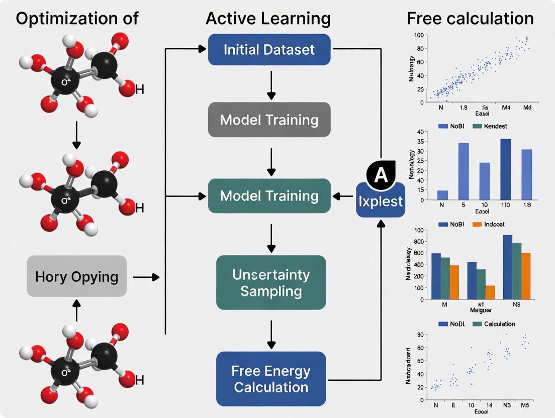
Standardized Workflow Diagram
The diagram below illustrates the logical flow and iterative nature of a standard Active Learning cycle for FEP.
Decision Guide for AL Protocol Tuning
This flowchart provides a systematic approach for diagnosing and resolving common performance issues in your AL-FEP setup.
The table below lists key computational tools and methodological components essential for setting up and running an AL-FEP workflow.
| Item / Resource | Function in AL-FEP Workflow | Notes |
|---|---|---|
| FEP Software (e.g., Flare FEP, FEP+ [1] [3]) | Generates high-accuracy binding affinity data for training the ML model. | The core physics-based simulation engine. Requires careful setup of force fields, water models, and simulation length [1]. |
| Machine Learning Model (e.g., 3D-QSAR [5]) | Learns from FEP data to make fast affinity predictions across the chemical library. | Model choice (e.g., Random Forests, Neural Networks) is often less critical than other AL parameters [2]. |
| Compound Library | The vast chemical space to be explored (e.g., bioisosteres, virtual compounds) [5]. | Can be generated via bioisostere replacement (e.g., using Spark) or virtual screening (e.g., using Blaze) [1]. |
| Acquisition Function | Balances exploration of new chemical space with exploitation of known potent regions. | Critical for selecting the next batch of compounds for FEP. Common functions include Upper Confidence Bound (UCB) and Expected Improvement (EI) [2] [4]. |
| High-Performance Computing (HPC) with GPUs | Provides the computational power to run multiple FEP calculations in parallel. | RBFE for a series of 10 ligands can take ~100 GPU hours; ABFE can take ~1000 hours [1]. |
Bridging Machine Learning and Physics-Based Simulations
Frequently Asked Questions (FAQs)
Q1: What is the most critical factor for success when applying Active Learning to Free Energy Perturbation (FEP) calculations? Research indicates that the number of molecules sampled in each Active Learning (AL) iteration is the most significant factor impacting performance. Sampling too few molecules per iteration can substantially hurt performance and prevent the model from effectively exploring the chemical space. In contrast, the study found AL performance to be largely insensitive to the specific machine learning method or acquisition function used [2].
Q2: My FEP calculations are not performing well with default settings for a particular target system. Is there an automated way to optimize the protocol? Yes, the FEP Protocol Builder (FEP-PB) tool addresses this exact problem. It uses an active learning workflow to iteratively search the protocol parameter space, automatically developing accurate FEP protocols for systems where default settings fail. This approach can generate robust protocols in a fraction of the time required for manual optimization [6].
Q3: How can I ensure my generative AI model produces synthesizable and novel molecules with high predicted affinity? Implement a nested active learning framework.
- Inner AL Cycle: Uses chemoinformatic oracles (drug-likeness, synthetic accessibility) to filter generated molecules.
- Outer AL Cycle: Uses physics-based oracles (molecular docking, free energy calculations) to evaluate and prioritize molecules with high predicted affinity. This iterative process allows the generative model to continuously refine its output based on feedback from both chemical and physical evaluators, successfully exploring novel chemical spaces for targets like CDK2 and KRAS [7].
Q4: What are the proven performance benchmarks for AL in free energy calculations? In an exhaustive study on a dataset of 10,000 congeneric molecules, under optimal AL conditions, researchers successfully identified 75% of the top 100 molecules by sampling only 6% of the full dataset. This demonstrates the profound efficiency gains achievable by optimizing the AL strategy for free energy calculations [2].
Troubleshooting Guides
Issue 1: Poor Performance of Default FEP Settings
Problem: Your FEP calculations for a specific target system are yielding inaccurate predictions and poor correlation with experimental data, even with established force fields and standard protocols.
Solution: Implement an Active Learning-based protocol optimizer.
| Step | Action | Objective | Key Parameter/Metric |
|---|---|---|---|
| 1 | Define Parameter Space | Identify tunable parameters in the FEP pipeline (e.g., simulation length, lambda spacing, force field options). | Creates a multidimensional search space. |
| 2 | Initial Sampling | Use the FEP-PB tool to select an initial set of protocol parameters for evaluation. | Establishes a baseline for model training. |
| 3 | Active Learning Loop | Iteratively run FEP calculations, evaluate performance, and select the next most informative protocols to test. | Minimizes total computational cost by focusing on high-potential protocols. |
| 4 | Protocol Validation | Apply the newly optimized protocol to a independent test set of molecules. | Validates predictive accuracy (target: ~1 kcal/mol error). |
This automated workflow rapidly generated accurate FEP protocols for challenging systems like MCL1 and p97, which were previously not amenable to calculations with default settings [6].
Issue 2: Generative Model Producing Impractical Molecules
Problem: Your generative AI model for molecular design produces molecules that are not synthesizable, have poor drug-likeness, or lack novelty (are too similar to known compounds).
Solution: Integrate a dual-cycle Active Learning framework to guide the generation process.
The following workflow diagram illustrates the nested AL cycles that iteratively refine molecule generation using chemoinformatic and physics-based oracles:
Key Checks and Actions:
- For Synthesizability: Integrate a synthetic accessibility (SA) score predictor as an oracle in the inner AL cycle. Molecules failing the SA threshold are discarded [7].
- For Novelty: In the inner cycle, calculate the similarity of generated molecules against the cumulative set of already-generated molecules. Prioritize molecules with lower similarity scores to explore new chemical space [7].
- For Target Engagement: Use physics-based oracles like molecular docking or absolute binding free energy (ABFE) calculations in the outer AL cycle to ensure generated molecules have a high predicted affinity for the biological target [7].
Issue 3: Active Learning Failing to Converge or Find Top Candidates
Problem: Your AL workflow is not efficiently identifying the best molecules in the chemical space, leading to slow convergence or sub-optimal results.
Solution: Systematically audit and optimize your AL design choices.
| Common Cause | Diagnostic Check | Corrective Action |
|---|---|---|
| Insufficient Batch Size | Check if performance plateaus or is unstable. Are too few molecules selected per iteration? | Increase the number of molecules sampled per AL iteration. This is the most critical factor. [2] |
| Poor Initial Sampling | Evaluate the diversity and representativeness of the initial training set. | Use a method like maximin or k-means++ for initial sample selection to ensure broad coverage of the chemical space. |
| Uninformative Acquisition Function | Analyze if the model is stuck in exploitation (only refining known areas) or exploration (random search). | Test different acquisition functions (e.g., UCB, EI, PI), though studies show this is less critical than batch size. Balance exploration vs. exploitation. [2] |
| Model Inaccuracy | Monitor the predictive model's error on a hold-out test set. | Ensure the machine learning model (e.g., Random Forest, Gaussian Process) is retrained with newly acquired data in each AL cycle. |
The Scientist's Toolkit: Research Reagent Solutions
The following table details key computational tools and methodologies central to integrating machine learning with physics-based simulations in drug discovery.
| Item Name | Function / Purpose | Key Application Note |
|---|---|---|
| FEP Protocol Builder (FEP-PB) | Automated tool that uses Active Learning to optimize parameters for Free Energy Perturbation calculations. | Critical for systems where default FEP settings fail. Rapidly generates predictive models for challenging targets like MCL1. [6] |
| VAE-AL Generative Workflow | A generative model (Variational Autoencoder) nested within Active Learning cycles for molecular design. | Generates novel, synthesizable, high-affinity molecules. Successfully applied to design CDK2 and KRAS inhibitors. [7] |
| Physics-Based Oracles | Molecular modeling methods (e.g., docking, absolute binding free energy calculations) used to evaluate generated molecules. | Provides a more reliable estimate of target engagement than data-driven methods alone, especially in low-data regimes. [7] |
| Chemoinformatic Oracles | Computational filters for drug-likeness (e.g., Lipinski's rules), synthetic accessibility, and molecular similarity. | Used in the inner AL cycle to ensure generated molecules are practical and novel. [7] |
| Active Learning Controller | The algorithm that selects the most informative data points (molecules or protocols) for the next round of evaluation. | Optimizing the batch size (molecules per iteration) is the most significant factor for achieving high performance. [2] |
Frequently Asked Questions
Q1: What are the most common causes of poor convergence in active learning cycles for free energy calculations? Poor convergence often stems from inadequate initial training data, poor collective variable (CV) selection, or insufficient sampling of rare binding events. To mitigate this, ensure your initial dataset, while small, is diverse and representative of the chemical space. For path-based methods, carefully choose CVs that accurately describe the binding pathway, as simple metrics like distance may fail for complex processes [8].
Q2: How can I balance the exploration of new chemical space with the exploitation of known hit compounds? Implement a balanced acquisition strategy. The ChemScreener workflow, for example, uses ensemble uncertainty to prioritize compounds predicted to be active while also selecting some molecules with high uncertainty to explore novel chemistry. This approach increased hit rates from 0.49% in primary screens to an average of 5.91% in case studies [9].
Q3: Our FEP+ protocol is not performing well for a challenging protein-ligand system. What steps should we take? Use a tool like FEP+ Protocol Builder, which employs an active learning workflow to iteratively search the protocol parameter space. This automates the optimization of settings for systems that do not work with default parameters, saving researcher time and increasing the success rate of FEP+ calculations [10].
Q4: What is the typical computational savings when using Active Learning Glide versus docking an entire ultra-large library? Active Learning Glide can recover approximately 70% of the top-scoring hits found by exhaustive docking while requiring only 0.1% of the computational cost and time [10].
Computational Performance Data
The following table summarizes key quantitative benefits of integrating active learning with free energy calculations, as demonstrated in recent research and commercial platforms.
| Method / Workflow | Key Performance Metric | Computational Savings / Efficiency Gain | Context / Library Size |
|---|---|---|---|
| Active Learning Glide [10] | Hit Recovery | ~70% of top hits recovered | Compared to exhaustive docking of ultra-large libraries (billions of compounds) |
| Active Learning Glide [10] | Cost & Time Reduction | 0.1% of compute cost and time | Achieved by docking only a fraction of the library |
| ChemScreener [9] | Hit Rate Enrichment | Increased from 0.49% (primary HTS) to avg. 5.91% | Five iterative screens on WDR5 protein (1,760 compounds tested) |
| Generative AI & Active Learning [11] | Lead Candidate Discovery | Lead candidate identified in 21 days | From generative AI to in vitro and in vivo testing |
| Physics-based & ML Screening [11] | Clinical Candidate Selection | Candidate selected after 10 months and 78 molecules synthesized | Computational screen of 8.2 billion compounds |
Detailed Experimental Protocols
Protocol 1: Active Learning Glide for Ultra-Large Virtual Screening
This protocol is designed to identify potent hits from billion-compound libraries using a combination of docking and machine learning [10].
- Library Preparation: Start with an ultra-large virtual library of readily accessible, drug-like small molecules [11].
- Initial Sampling: Perform physics-based molecular docking (e.g., with Glide) on a small, randomly selected subset of the library (e.g., 0.01%).
- Model Training & Prediction: Train a machine learning (ML) model on the docking scores and molecular descriptors from the initial set. Use this model to predict scores for the entire unscreened library.
- Iterative Batch Selection: Select the next batch of compounds based on a balanced acquisition function (e.g., prioritizing both high predicted scores and high model uncertainty). Dock this new batch.
- Model Update & Convergence: Incorporate the new docking results into the training data and update the ML model. Repeat steps 4 and 5 until the top-ranking compounds stabilize or a predefined number of iterations is reached.
- Output: A final list of top-scoring compounds, recovering a high percentage of the hits that would have been found by a prohibitively expensive exhaustive dock.
Protocol 2: ChemScreener's Multi-Task Active Learning for Hit Discovery
This protocol is tailored for early drug discovery with limited initial data, using multi-task learning and a balanced-ranking strategy [9].
- Assay Design & Initialization: Establish a primary high-throughput screening assay (e.g., HTRF). Begin with a small, diverse set of compounds for initial testing.
- Multi-Task Model Training: Train an ensemble of deep learning models on the initial bioactivity data. The "multi-task" aspect allows the model to learn from related assays or general molecular properties.
- Balanced-Ranking Acquisition: For each subsequent screening cycle, rank the remaining compounds in the library using an acquisition function that balances:
- Exploitation: Selecting compounds with the highest predicted activity.
- Exploration: Selecting compounds where the model's predictions have the highest uncertainty (ensemble disagreement).
- Iterative Screening & Model Retraining: Screen the selected compounds (e.g., 352 compounds per cycle in the WDR5 study). Add the new experimental results to the training data and retrain the model.
- Hit Validation & Progression: After several cycles, consolidate hits and their close analogs. Validate confirmed hits in secondary and counter-screens (e.g., dose-response, DSF for binding confirmation). Advance diverse scaffold series for further development.
Workflow and Pathway Visualizations
Active Learning Docking Cycle
Integrated Drug Discovery Workflow
The Scientist's Toolkit: Research Reagent Solutions
| Item / Resource | Function in the Workflow |
|---|---|
| Ultra-Large Virtual Libraries (e.g., ZINC20, GDB-17-derived) [11] | Billions of "on-demand" synthesizable compounds provide the vast chemical space for virtual screening. |
| Molecular Docking Software (e.g., Glide) [10] | Provides the initial, physics-based binding affinity scores for compounds used to train the active learning model. |
| Free Energy Perturbation (FEP+) Software [10] | Offers high-accuracy binding affinity predictions for lead optimization, used to validate and refine hits from initial screens. |
| Path Collective Variables (PCVs) [8] | Sophisticated collective variables used in path-based free energy calculations to map the protein-ligand binding pathway accurately. |
| Balanced-Ranking Acquisition Function [9] | The algorithm that decides which compounds to test next, balancing the need to find active compounds (exploit) and learn about the chemical space (explore). |
Core Concepts: Exploitation and Exploration
In Active Learning (AL), the exploration-exploitation trade-off is a fundamental challenge. The goal is to use a limited labeling budget to query the most informative data points from a pool of unlabeled data.
- Exploitation aims to maximize a domain-specific objective given the current knowledge of the model. In drug discovery, this often means selecting compounds predicted to have the highest binding affinity to a target protein. This is also known as a greedy acquisition strategy [12].
- Exploration focuses on reducing the uncertainty of the learning model itself. This involves selecting data points where the model's prediction is most uncertain, thereby improving the model's overall understanding of the underlying data distribution [13] [12].
A balanced approach is often necessary. Purely exploitative strategies might miss more potent compounds in unexplored chemical spaces, while purely exploratory strategies may be inefficient for directly optimizing the desired objective, such as finding the highest-affinity binder [13] [12].
The following diagram illustrates a general AL workflow that can incorporate both exploitative and exploratory strategies:
Frequently Asked Questions & Troubleshooting
1. How do I choose between an exploitative or exploratory strategy for my FEP project?
The optimal choice depends on your project's stage and goals.
- Use an exploitative (greedy) strategy when you are in later stages of lead optimization and have a reasonably accurate model. This focuses resources on the most promising regions of chemical space to find the best candidates quickly [12].
- Use an exploratory (uncertainty) strategy in the early stages of a project or when exploring a new chemical series. This helps build a robust and generalizable model by sampling diverse structures [12].
- Use a balanced strategy to avoid the pitfalls of either extreme. For example, a "narrowing" strategy starts with broad exploration for the first few AL iterations before switching to exploitation, which has been shown to efficiently identify potent binders [12].
2. My AL model seems to get stuck in a local optimum, repeatedly selecting similar compounds. What should I do?
This is a common issue with overly exploitative strategies. To encourage more diversity in selected compounds:
- Incorporate exploration explicitly: Switch to an uncertainty-based acquisition function or use a mixed strategy that selects some candidates based on high uncertainty [12].
- Adjust the batch size: Select more compounds per AL iteration. Research has shown that using larger batch sizes (e.g., 60-100 molecules per iteration) significantly improves the recall of top binders by ensuring better coverage of the chemical space in each cycle [2].
- Use molecular descriptors that capture diversity: Ensure your model uses descriptors like molecular fingerprints (e.g., from RDKit) that effectively represent the chemical space. These have been shown to outperform other descriptors for broadly exploring the chemical library [12].
3. What is the impact of the initial training set on the AL process?
The initial set of labeled data is critical.
- Problem: A small or non-representative initial set can lead the model to make poor predictions from the start, causing the AL strategy to query suboptimal candidates.
- Solution: If possible, start with an initial dataset that provides broad coverage of the chemical space you intend to explore. Some methods use clustering or density-based sampling on the unlabeled pool to select a diverse initial set [13].
Experimental Protocols for AL in Free Energy Calculations
The table below summarizes a generalized protocol for implementing an AL cycle to optimize compounds using free energy calculations.
- Goal: To efficiently identify high-affinity ligands by guiding the selection of compounds for costly RBFE calculations.
- Surrogate Model: A Quantitative Structure-Activity Relationship (QSAR) model that predicts binding affinity based on molecular features [12].
| Protocol Step | Key Details & Considerations |
|---|---|
| 1. Initial Setup | Define your chemical library. Select an initial training set of compounds with known binding affinities (from experiments or preliminary FEP calculations). Train the initial QSAR model [12]. |
| 2. Iterative Active Learning Cycle | |
| a. Model Prediction | Use the current QSAR model to predict binding affinities and their uncertainties for all compounds in the unlabeled pool [12]. |
| b. Acquisition Function | Apply the chosen strategy (e.g., greedy, uncertainty, or mixed) to select the next batch of compounds for FEP calculation. A common practice is to select the top 20 predicted binders from each of the best-performing models [12]. |
| c. Experiment (FEP Calculation) | Perform RBFE calculations on the selected compounds. This provides the "ground truth" labels for the model [12] [14]. |
| d. Model Update | Add the new FEP data to the training set. Retrain the QSAR model to incorporate the new knowledge [12]. |
| 3. Termination & Validation | Stop when a stopping criterion is met (e.g., a sufficient number of high-affinity binders have been identified, or model performance plateaus). Synthesize and experimentally test the top-predicted compounds [14]. |
The Scientist's Toolkit: Research Reagents & Materials
This table lists key computational "reagents" and tools used in building an AL framework for free energy calculations.
| Item | Function in the Experiment |
|---|---|
| Chemical Library | A virtual collection of compounds to be screened. This is the search space from which the AL algorithm selects candidates [12]. |
| Molecular Descriptors/Fingerprints | Numerical representations of chemical structure (e.g., RDKit fingerprints, PLEC fingerprints). These are the input features for the QSAR model [12]. |
| Surrogate QSAR Model | A machine learning model (e.g., Random Forest, Gaussian Process) that learns the relationship between molecular features and binding affinity. It provides fast predictions to guide the AL cycle [12]. |
| Acquisition Function | The algorithm that balances exploration and exploitation to decide which compounds to test next. Examples include greedy, uncertainty, and expected improvement [13] [12]. |
| FEP/RBFE Calculation Engine | The physics-based simulation software (e.g., Schrodinger's FEP+, OpenMM) that provides high-accuracy binding affinity data for the selected compounds, used to label data and validate predictions [14]. |
Implementing AL-FEP: Workflows, Tools, and Real-World Case Studies
The AL-FEP (Active Learning for Free Energy Perturbation) workflow integrates advanced computational simulations with an iterative learning loop to optimize compounds, such as antibodies or small molecules, for properties like binding affinity. This method efficiently navigates vast chemical spaces by prioritizing the most promising candidates for computationally expensive calculations [1] [15].
The following diagram illustrates the core cyclic process of the AL-FEP workflow.
Troubleshooting Guides
Problem 1: Poor Prediction Accuracy from the Surrogate Model
Issue: The surrogate model's predictions do not correlate well with subsequent high-cost FEP calculations.
| Potential Cause | Diagnostic Steps | Recommended Solution |
|---|---|---|
| Insufficient or poor-quality initial data | Check the size and diversity of the starting dataset. | Start with a minimum of 10-20 diverse compounds with reliable affinity data. Use clustering to ensure structural diversity [15]. |
| Inadequate representation of molecules | Evaluate the feature set or embeddings used for the model. | Use a protein Language Model (pLM) to generate sequence embeddings, capturing complex biophysical properties [15]. |
| Model overfitting | Plot learning curves to see if validation performance plateaus or worsens. | Employ Parameter-Efficient Fine-Tuning (PEFT). This adapts a large pLM to your specific task with limited data, reducing overfitting risk [15]. |
Problem 2: High Computational Cost and Slow Workflow Iteration
Issue: The time and resources required for each AL-FEP cycle are prohibitive.
| Potential Cause | Diagnostic Steps | Recommended Solution |
|---|---|---|
| Standard FEP calculations are too expensive | Profile the computation time of a single FEP simulation. | Implement an automated lambda window scheduling algorithm. This avoids calculating too many or too few windows, optimizing GPU time [1]. |
| Inefficient candidate selection | Review the number of candidates evaluated by FEP in each cycle. | Use the surrogate model to score a large virtual library, but only run FEP on the top 5-10% of candidates that are also "informative" for the model [15]. |
| Overly large molecular systems | Check the number of atoms in the simulated system (e.g., protein, membrane, water). | For membrane-bound targets (like GPCRs), test if truncating distant parts of the protein system significantly impacts results, as this can drastically reduce simulation time [1]. |
Problem 3: Handling Charged Ligands and Hydration Effects
Issue: FEP calculations involving formal charge changes or specific water molecules yield unreliable results with high hysteresis.
| Potential Cause | Diagnostic Steps | Recommended Solution |
|---|---|---|
| Charge changes in perturbations | Identify if ligands in the perturbation map have different formal charges. | Introduce a counterion to neutralize the charged ligand, keeping the net formal charge consistent across the simulation. Run longer simulation times for these transformations to improve reliability [1]. |
| Inconsistent hydration environment | Check for high hysteresis between forward and reverse transformations in a perturbation. | Use hydration analysis techniques like 3D-RISM or GIST to identify poorly hydrated regions. Employ sampling methods like GCNCMC to ensure stable and consistent water placement during the simulation [1]. |
Problem 4: Optimized Compounds Have Poor Developability
Issue: The workflow successfully improves binding affinity (e.g., lowers Flex ddG energy) but yields compounds with undesirable properties for therapeutics.
| Potential Cause | Diagnostic Steps | Recommended Solution |
|---|---|---|
| Single-objective optimization | The optimization target is solely binding affinity. | Implement multi-objective optimization. Incorporate metrics like AbLang2 perplexity (to maintain "natural" antibody sequence traits), hydropathicity, and instability index as simultaneous optimization goals [15]. |
Frequently Asked Questions (FAQs)
Q1: What is the fundamental difference between Relative Binding Free Energy (RBFE) and Absolute Binding Free Energy (ABFE), and when should I use each?
- RBFE calculates the binding energy difference between two similar ligands. It is highly accurate for congeneric series but is typically limited to perturbations involving a small number of atom changes (e.g., ~10 atoms). It is best suited for lead optimization where you are making small, systematic changes to a molecule [1].
- ABFE calculates the absolute binding energy of a single ligand independently. It is not restricted by the need for similar ligands, making it ideal for virtual screening and hit identification where molecules can be structurally diverse. However, ABFE calculations are computationally more demanding (~10x more GPU hours than RBFE) and may have residual errors due to unaccounted protein conformational changes [1].
Q2: How does Active Learning specifically improve upon a standard FEP workflow?
Standard FEP might involve running calculations on a large, pre-defined set of compounds. Active Learning introduces an intelligent, iterative cycle. A surrogate model selects the most "informative" compounds for the next round of FEP calculations, balancing exploration of uncertain regions of chemical space with exploitation of known high-affinity areas. This means you can achieve better results with far fewer expensive FEP calculations compared to a brute-force approach [15].
Q3: My project involves covalent inhibitors. Can the AL-FEP workflow handle them?
Modeling covalent inhibitors is challenging because it requires specialized force field parameters to correctly describe the bond formation between the ligand and the protein. Standard force fields often lack these parameters. While industry-wide efforts are ongoing to develop reliable methods, you should currently approach covalent systems with caution and be prepared to invest significant effort in parameterization [1].
Q4: What are the minimum computational resources required to start with an AL-FEP project?
A typical RBFE study for a congeneric series of about 10 ligands might require approximately 100 GPU hours. In contrast, an equivalent ABFE study would be far more demanding, likely requiring around 1000 GPU hours. The exact needs depend on system size, simulation length, and the number of compounds evaluated [1].
Experimental Protocols
Protocol 1: Setting Up a Relative Binding Free Energy (RBFE) Calculation
This protocol details the steps for a standard RBFE calculation between two similar ligands [1].
- System Preparation:
- Obtain the 3D structures of the protein and both ligands (Ligand A and Ligand B).
- Ensure both ligands are in the same protonation state. If formal charges differ, add a neutralizing counterion.
- Parameterize the ligands using a force field like Open Force Field (OpenFF), and check for any poorly described torsion angles that may require optimization using Quantum Mechanics (QM) calculations.
- Perturbation Map Generation:
- Define the transformation from Ligand A to Ligand B. An automated tool is often used to map the atoms between the two molecules.
- Use an automated lambda window scheduling algorithm to determine the optimal number of intermediate steps (windows) for the transformation. This prevents wasted computational effort.
- Simulation Setup:
- Set up the simulation boxes for both the bound (protein-ligand complex) and unbound (ligand in solvent) states for both endpoints.
- For transformations involving charge changes, plan for longer simulation times to ensure proper equilibration.
- Production Run and Analysis:
- Run the molecular dynamics simulations for each lambda window.
- Use analysis software (e.g., built-in tools in software like Flare FEP, Schrodinger's FEP+, OpenFE) to calculate the relative free energy difference (ΔΔG) between Ligand A and Ligand B.
Protocol 2: Incorporating Active Learning for Multi-Objective Optimization
This protocol extends a standard FEP workflow with an Active Learning loop for balancing affinity and developability [15].
- Initialization:
- Start with a wild-type antibody sequence and a small set of known variant sequences with measured binding affinity data.
- Fine-tune a protein Language Model (pLM) on this initial data using Parameter-Efficient Fine-Tuning (PEFT) and a learning-to-rank objective. This creates your initial surrogate model.
- Candidate Generation and Selection:
- Generate candidate sequences by sampling directly from the probability distribution of the fine-tuned pLM.
- For each candidate, calculate multiple objective scores:
- Predicted Binding Affinity: From the surrogate model.
- AbLang2 Perplexity: Measures how "natural" the antibody sequence is.
- Developability Metrics: Calculate hydropathicity, instability index, and isoelectric point from the sequence.
- Select the next set of compounds for FEP evaluation using a multi-objective selection criterion like hypervolume maximization, which balances all these objectives.
- Iteration:
- Run FEP (or a cheaper proxy like Flex ddG) on the selected compounds to obtain a more reliable binding affinity score.
- Add the new data (sequence and measured affinity) to the training set.
- Update (fine-tune) the surrogate model with the expanded dataset.
- Repeat steps 2 and 3 until a stopping criterion is met (e.g., no further improvement after several cycles or a target affinity is reached).
The Scientist's Toolkit: Research Reagent Solutions
| Item/Resource | Function in AL-FEP Workflow | Key Considerations |
|---|---|---|
| Open Force Field (OpenFF) Initiative | Provides accurate, chemically transferable force fields for small molecules, essential for correctly modeling ligand energetics and dynamics [1]. | Check for parameter coverage for novel functional groups or metal ions in your system. |
| Protein Language Models (pLMs) | Acts as a pre-trained surrogate model; generates meaningful embeddings for protein/antibody sequences and can be fine-tuned for fitness prediction with limited data [15]. | Models like AbLang2 are specifically trained on antibody sequences (OAS database) and are ideal for antibody engineering projects [15]. |
| Grand Canonical Monte Carlo (GCNCMC) | A sampling technique that allows water molecules to be inserted and deleted during simulation, ensuring the binding site is correctly and consistently hydrated [1]. | Critical for reducing hysteresis in RBFE calculations where water displacement or rearrangement is a key factor. |
| Automated Lambda Scheduler | Dynamically determines the optimal number and spacing of intermediate states (lambda windows) for a given alchemical transformation [1]. | Prevents both inaccurate results (too few windows) and wasted computational resources (too many windows). |
| Active Learning Framework (e.g., ALLM-Ab) | Provides the algorithmic backbone for the iterative cycle of selection, evaluation, and model updates. Manages the trade-off between exploration and exploitation [15]. | Look for frameworks that support multi-objective optimization to balance affinity with developability early in the design process. |
FEgrow is an open-source Python package designed to build and optimize congeneric series of ligands directly within a protein's binding pocket [16]. Its primary role in structure-based drug design is to address a critical bottleneck: the creation of reliable initial binding poses for ligands, which is a fundamental prerequisite for successful free energy calculations [16] [17]. By growing user-defined R-groups from a constrained core of a known hit compound, FEgrow maximizes the use of structural biology data and incorporates medicinal chemistry expertise, thereby reducing reliance on less accurate docking algorithms [16] [18].
This case study frames the use of FEgrow within a broader thesis on optimizing active learning for free energy calculations research. The integration of active learning allows for a more efficient exploration of the vast combinatorial space of possible chemical groups, significantly accelerating the hit identification and optimization process [19] [18]. We will demonstrate its application in targeting the SARS-CoV-2 Main Protease (Mpro), a key viral replication enzyme and a prominent drug target [20].
Research Reagent Solutions
The following table details the essential computational tools and data required to set up and run an FEgrow experiment for Mpro inhibitor optimization.
| Resource Name | Type/Source | Function in the Workflow |
|---|---|---|
| Protein Data Bank (PDB) | Database (e.g., PDB ID: 7EN8) | Source of the initial receptor structure (SARS-CoV-2 Mpro) and a known ligand-core complex [21]. |
| Ligand Core | User-defined (from a known hit) | The central scaffold whose binding mode is fixed during R-group growth [16] [18]. |
| R-group Library | FEgrow (provided ~500 groups) or user-defined | A collection of functional groups to be grown from the core's attachment point [16]. |
| Linker Library | FEgrow (provided ~2000 linkers) | A collection of flexible chemical linkers to connect the core and R-group [18]. |
| RDKit | Software Library | Handles core merging, conformer generation (ETKDG method), and maximum common substructure search [16] [18]. |
| OpenMM | Software Library | Performs structural optimization of ligand conformers within a rigid protein using molecular mechanics [18]. |
| ANI Neural Network Potential | Machine Learning Potential | Provides accurate intramolecular energetics for the ligand during optimization (hybrid ML/MM) [16]. |
| gnina | Software Tool | A convolutional neural network used to score and predict binding affinities of the low-energy poses [16] [18]. |
The process of building and optimizing ligands with FEgrow follows a structured, modular pathway. The diagram below illustrates the key stages from input preparation to final output.
FEgrow in Action: SARS-CoV-2 Mpro Case Study
Experimental Protocol for Mpro Inhibitor Elaboration
A typical FEgrow experiment to optimize Mpro inhibitors involves the following detailed methodology [16] [18]:
System Preparation:
- Receptor: Obtain the crystal structure of SARS-CoV-2 Mpro (e.g., PDB code 7EN8). Prepare the protein structure by adding hydrogen atoms and assigning protonation states at pH 7 using software like Open Babel. The key catalytic dyad residues are Cys145 and His41 [20].
- Ligand Core: Define the core scaffold from a known inhibitor (e.g., a fragment from a crystallographic screen). The core must include a specified hydrogen atom as the attachment point for growth.
Ligand Building and Conformer Generation:
- Select an R-group from the provided library or a custom list. A linker from the library can also be chosen to connect the core and R-group.
- FEgrow uses RDKit to merge the core and R-group/linker at the defined attachment point.
- An ensemble of 3D conformers for the new ligand is generated using the ETKDG algorithm. Crucially, harmonic distance restraints (with a force constant of 10^4 kcal/mol/Ų) are applied to atoms in the common core to maintain the original bioactive conformation [16].
Conformer Optimization and Scoring:
- Generated conformers are filtered to remove any that sterically clash with the rigid protein binding pocket.
- The remaining conformers undergo structural optimization via energy minimization in OpenMM. In a hybrid ML/MM approach, the ligand's intramolecular energetics are described by the ANI machine learning potential, while its non-bonded interactions with the static protein are handled by a classical force field (AMBER FF14SB for the protein) [16] [18].
- The low-energy optimized structures are scored using the
gninaconvolutional neural network scoring function to predict binding affinity [18].
Active Learning Integration (Advanced Workflow):
- To efficiently search the vast combinatorial space of linkers and R-groups, the workflow can be interfaced with an active learning cycle [19] [18].
- A batch of compounds is grown, built, and scored with FEgrow.
- The results train a machine learning model, which then predicts the scores for the remaining unexplored chemical space.
- The next batch of compounds is selected based on the model's predictions, iteratively improving the quality of designs while minimizing computational cost [18].
Troubleshooting Common Experimental Issues
FAQ 1: My grown conformers consistently show high energy or steric clashes after optimization. What steps can I take?
- A: This is often related to the initial conformer generation or the optimization parameters.
- Check Core Restraints: Verify that the atoms of the ligand core are correctly identified and strongly restrained during conformer generation. This ensures the known binding mode is preserved.
- Adjust Conformer Sampling: Increase the number of conformers generated by the ETKDG algorithm to better sample the rotational space of the added R-group and linker.
- Review Optimization Parameters: Ensure the hybrid ML/MM potential is correctly configured. The ANI potential for the ligand provides a more accurate energy surface for unusual chemistries compared to traditional force fields [16].
FAQ 2: The gnina scoring function ranks a compound as high-affinity, but subsequent free energy calculations suggest poor binding. What could be the cause?
- A: Discrepancies between different scoring methods are not uncommon.
- Pose Reliability: The gnina score is dependent on the input pose. Verify that the optimized pose from FEgrow is physically reasonable by visually inspecting key interactions (e.g., with the S1/S2 pockets of Mpro and the catalytic dyad).
- Scoring Function Limitations: Remember that gnina is a docking-style scoring function. It is excellent for rapid screening but is an approximation. Use it for relative ranking within a congeneric series, not as an absolute predictor of affinity [16] [18].
- Input for Free Energy Calculations: Ensure the structures output by FEgrow have been properly prepared (e.g., parameterized) for the subsequent free energy calculation software (e.g., SOMD) [16].
FAQ 3: How can I integrate purchasable compounds from on-demand libraries into my FEgrow active learning campaign?
- A: This is a powerful feature for ensuring synthetic tractability.
- Seed Chemical Space: The FEgrow workflow can be configured to "seed" the initial or subsequent batches of the active learning cycle with molecules from on-demand libraries (e.g., the Enamine REAL database) that contain the defined core substructure [18].
- Treat as Flexible: In this mode, the entire molecule outside of the rigid core is treated as flexible during the FEgrow building and optimization process, allowing you to evaluate purchasable analogs directly [18].
Results and Validation
Key Findings from Prospective Application
In a prospective study targeting SARS-CoV-2 Mpro, researchers used the active learning-driven FEgrow workflow to prioritize 19 compound designs for purchase and experimental testing [19] [22] [18]. The results were promising:
- Hit Rate: Three of the 19 tested compounds showed weak but detectable activity in a fluorescence-based Mpro enzyme assay, validating the workflow's ability to generate biologically active molecules [18].
- Validation of Design Strategy: The study also demonstrated that the fully automated workflow could identify novel designs with high similarity to potent inhibitors discovered by the open-science COVID Moonshot effort, using only initial fragment screen data [18].
Performance of Optimized Workflow
The integration of active learning with FEgrow represents a significant performance enhancement. The table below summarizes the key metrics of this optimized workflow.
| Workflow Component | Performance Metric | Outcome/Benefit |
|---|---|---|
| Automation & Parallelization | Throughput of compound building and scoring | Enabled automated de novo design on HPC clusters via a new API [18]. |
| Active Learning | Search efficiency in combinatorial chemical space | Identified promising inhibitors by evaluating only a fraction of the total space, reducing computational cost [18]. |
| On-demand Library Seeding | Synthetic tractability of final designs | Directly generated suggestions for purchasable compounds (e.g., from Enamine REAL database), bridging virtual design and real-world testing [18]. |
This case study demonstrates that FEgrow is a robust, open-source platform for optimizing lead compounds within a protein binding pocket, effectively preparing them for rigorous free energy calculations. Its application to SARS-CoV-2 Mpro inhibitor design, especially when coupled with an active learning framework, provides a validated blueprint for accelerating early-stage drug discovery [16] [18]. The successful identification of active Mpro inhibitors underscores the value of combining structural biology data, hybrid ML/MM optimization, and machine-learning-driven search strategies.
Future developments in FEgrow will likely focus on incorporating a wider array of optimization algorithms and scoring functions, further enhancing its accuracy and flexibility [18]. For the computational drug discovery community, adopting and contributing to such open-source, modular tools is crucial for advancing the field of free energy calculations and achieving more predictive, efficient, and reliable molecular design.
Experimental Workflow & Methodology
Core Generative AI and Active Learning Workflow
Our established methodology integrates a generative variational autoencoder (VAE) with a physics-based active learning (AL) framework to design novel inhibitors [7]. The workflow consists of several interconnected stages, as illustrated below.
Diagram 1: Generative AI with Nested Active Learning Workflow
Key Experimental Steps [7]:
Data Representation & Initial Training:
- Represent training molecules as tokenized SMILES strings converted into one-hot encoding vectors.
- Pre-train the VAE on a general molecular dataset to learn viable chemical structures.
- Fine-tune the VAE on a target-specific training set (e.g., known CDK2 or KRAS binders) to increase initial target engagement.
Nested Active Learning Cycles:
- Inner AL Cycle (Chemoinformatics Oracle): Generated molecules are evaluated for drug-likeness, synthetic accessibility (SA), and novelty (dissimilarity from training set). Molecules meeting predefined thresholds are added to a temporal-specific set and used to fine-tune the VAE.
- Outer AL Cycle (Affinity Oracle): After several inner cycles, accumulated molecules undergo molecular docking. Those with favorable docking scores are promoted to a permanent-specific set, which is used for subsequent VAE fine-tuning, directly steering generation toward high-affinity candidates.
Candidate Selection:
Key Quantitative Results from the CDK2 Case Study
The application of this workflow for CDK2 inhibitor discovery yielded the following experimental outcomes [7]:
Table 1: Experimental Validation of Generated CDK2 Inhibitors
| Metric | Result | Experimental Method |
|---|---|---|
| Molecules Synthesized | 9 | Chemical synthesis |
| Molecules with in vitro activity | 8 | Bioassay |
| Molecules with nanomolar potency | 1 | Dose-response bioassay |
| Novel scaffolds generated | Multiple, distinct from known CDK2 inhibitors | Chemical similarity analysis |
Frequently Asked Questions (FAQs) & Troubleshooting
On Generative Model Performance
Q1: Our generative model produces molecules with poor synthetic accessibility (SA). How can we improve this?
- Problem: The VAE decoder generates chemically invalid or highly complex structures.
- Solution: Integrate a synthetic accessibility (SA) predictor as a filter within the Inner AL Cycle. Molecules with poor SA scores should be rejected before fine-tuning. This iteratively teaches the VAE to prioritize synthetically feasible structures [7]. Reinforce the generation with SA-focused reward functions if using reinforcement learning.
Q2: The generated molecules lack novelty and are too similar to the training set.
- Problem: The model suffers from mode collapse or fails to explore new chemical space.
- Solution: Actively promote dissimilarity during the AL cycles. In the inner cycle, enforce a minimum Tanimoto dissimilarity threshold against the cumulative set of previously generated molecules. This explicitly penalizes the generation of redundant structures and encourages exploration [7].
On Active Learning and Free Energy Calculations
Q3: How can we configure the AL cycles for targets with very little training data, like KRAS?
- Problem: Sparse target-specific data limits the initial model's ability to generate active compounds.
- Solution: Leverage the physics-based oracles in the outer cycle. For low-data targets like KRAS, the docking score oracle provides a critical, reliable guide that is less dependent on existing bioactivity data. Extend the initial pre-training phase on a larger, general bioactivity corpus before fine-tuning on the small target-specific set [7].
Q4: Our free energy calculations are unstable or show poor convergence. What are the key parameters to check?
- Problem: Unreliable Absolute Binding Free Energy (ABFE) or Thermodynamic Integration (TI) results.
- Solution: Follow these practical guidelines derived from optimized protocols [24] [23]:
- Restraint Selection: Use an algorithm that incorporates protein-ligand hydrogen bonds to choose pose restraints, improving numerical stability and convergence [23].
- Simulation Length: For TI, sub-nanosecond simulations can be sufficient for many systems, but some (e.g., TYK2) may require longer equilibration (~2 ns) [24].
- Perturbation Size: Avoid large perturbations with |ΔΔG| > 2.0 kcal/mol, as they exhibit significantly higher errors [24].
- Annihilation Protocol & Scaling: Optimize the ligand annihilation protocol and the order in which interactions (electrostatics, Lennard-Jones, restraints) are scaled to minimize error and improve precision [23].
Q5: How can we use free energy calculations to optimize kinome-wide selectivity?
- Problem: A lead compound is potent but inhibits many off-target kinases.
- Solution: Implement a hierarchical selectivity profiling strategy using free energy calculations [14]:
- Use Ligand-based Relative Binding Free Energy (L-RB-FEP+) calculations to predict potency against the primary target (e.g., Wee1) and key off-targets (e.g., PLK1).
- Employ Protein Residue Mutation Free Energy (PRM-FEP+) calculations. This efficiently estimates the impact of mutating a "selectivity handle" residue in your primary target (e.g., the gatekeeper residue) to match the sequence of various off-target kinases, approximating binding across the kinome without simulating every individual off-target structure [14].
On Biological Context and Validation
Q6: What are the relevant cellular pathways and biomarkers for CDK2 and KRAS inhibition?
The diagrams below summarize the key signaling pathways and cellular responses for the two targets.
Diagram 2: Core Oncogenic KRAS Signaling Pathway [25]
Diagram 3: Cellular Context Determines Response to CDK2 Inhibition [26]
Q7: How can we validate the mechanism of action and address potential resistance?
- For KRAS: In pancreatic ductal adenocarcinoma (PDAC) models, combination therapy is often essential. KRAS inhibition (e.g., with MRTX1133) can reverse chemotherapy resistance promoted by therapy-induced senescence. Combining KRASG12D inhibition with gemcitabine reduces senescence-associated β-galactosidase (SA-β-gal) signal and sensitizes cells to treatment [27].
- For CDK2: Response is highly context-dependent. Use biomarkers like P16INK4A loss and Cyclin E1 overexpression to identify models sensitive to pure G1 arrest. In CDK2-independent models, inhibitors may induce a 4N arrest; in these cases, combination strategies, such as with CDK4/6 inhibitors or depletion of mitotic regulators, can be effective [26]. CRISPR screens have identified CDK2 loss as a mechanism of resistance, underscoring the need for combination therapies [26].
The Scientist's Toolkit: Research Reagent Solutions
Table 2: Essential Computational and Experimental Reagents
| Item / Reagent | Function / Role in Workflow | Example / Note |
|---|---|---|
| Variational Autoencoder (VAE) | Core generative model; maps molecules to latent space and generates novel structures. | Balances rapid sampling, interpretable latent space, and stable training [7]. |
| SMILES Representation | Standardized string-based molecular representation for model input. | Requires tokenization and one-hot encoding [7]. |
| Chemoinformatic Oracles | Filters in the Inner AL Cycle for drug-likeness and synthetic accessibility (SA). | Critical for ensuring generated molecules are synthesizable and have drug-like properties [7]. |
| Molecular Docking | Physics-based affinity oracle in the Outer AL Cycle for initial affinity assessment. | Provides a rapid, structure-based score to prioritize molecules [7]. |
| PELE (Protein Energy Landscape Exploration) | Advanced simulation for refining binding poses and assessing stability. | Used for in-depth evaluation of protein-ligand complexes before synthesis [7]. |
| ABFE (Absolute Binding Free Energy) Calculations | High-accuracy prediction of binding affinity for final candidate selection. | Optimized protocols are crucial for stability and convergence [23]. |
| Thermodynamic Integration (TI) | A specific method for relative binding free energy calculations. | An automated workflow using AMBER20 and alchemlyb can be implemented [24]. |
| MRTX1133 | Experimental non-covalent KRASG12D inhibitor. | Used in vitro to validate KRAS targeting and combination strategies [27]. |
| Gemcitabine | Standard chemotherapy agent for pancreatic cancer. | Used in combination studies with KRAS inhibitors to overcome resistance [27]. |
Integrating AL into Existing FEP Pipelines
Free Energy Perturbation (FEP) is a physics-based computational technique renowned for its high accuracy in predicting protein-ligand binding affinities, a critical task in rational drug design. [3] However, its computational expense and low throughput have traditionally limited its application to smaller congeneric series, typically involving perturbations of fewer than 10 atoms. [28] Active Learning (AL) is a machine learning strategy that addresses this bottleneck. By iteratively selecting the most informative compounds for costly FEP calculations, AL creates a feedback loop that efficiently explores vast chemical spaces, making FEP a powerful tool for earlier stages of drug discovery, such as hit identification and large-scale library profiling. [1] [3]
This guide provides troubleshooting and best practices for researchers integrating AL into their FEP workflows.
Frequently Asked Questions (FAQs)
Q1: What is the fundamental difference between a standard FEP workflow and an Active Learning FEP workflow?
A standard FEP workflow is typically a single-shot calculation on a pre-defined, congeneric set of ligands. In contrast, an Active Learning FEP workflow is an iterative cycle. It starts with an initial set of FEP calculations on a small, diverse subset of a larger compound library. A machine learning model (like a 3D-QSAR model) is trained on this FEP data and is then used to rapidly predict the binding affinities for the entire remaining library. The most promising or uncertain compounds from this large set are then selected for the next round of FEP calculations. This process repeats, with the model being retrained each time, continuously refining its predictions and guiding the exploration of chemical space. [1]
Q2: My Active Learning model is not improving after the first few iterations. What could be wrong?
This is a common challenge, often referred to as model stagnation.
- Lack of Diversity in Initial Training Set: If the initial compounds used for the first FEP cycle are too similar, the ML model cannot learn the broader structure-activity relationships (SAR) of the chemical space. Ensure your initial selection is chemically diverse.
- Exploration vs. Exploitation Imbalance: The selection strategy for the next FEP batch might be too greedy, only picking compounds predicted to be the very best (exploitation). Incorporate strategies that also select compounds where the model is most uncertain (exploration) to improve the model in under-sampled regions.
- Inaccurate FEP Ground Truth: The entire AL cycle relies on the accuracy of the FEP calculations. If the initial FEP results are unreliable due to protein structure issues, incorrect protonation states, or poor ligand poses, the ML model will learn from noisy or incorrect data. Always validate your FEP setup with known experimental data first. [1]
Q3: Can Active Learning FEP handle charged ligands or large conformational changes in the binding site?
This remains a significant challenge. Standard Relative FEP (RBFE), which is often used in AL cycles, struggles with formal charge changes due to numerical issues, though recent advances allow it by using counterions and longer simulation times. [1] Furthermore, most FEP methods treat the protein as largely rigid, meaning they cannot sample large backbone or loop movements. If your ligand series induces different protein conformations, they should be treated in separate FEP experiments. [28] For these complex cases, Absolute FEP (ABFE) might be considered, as it allows the use of different protein structures for different ligands, but it is computationally much more demanding. [1]
Q4: What are the key metrics to monitor for a successful Active Learning FEP campaign?
Monitor both the performance of the FEP calculations and the ML model:
- FEP Metrics: Hysteresis (the difference between forward and reverse transformations) should be low (< 1 kcal/mol), and calculated free energies should match experimental values for known compounds (root-mean-square error, or RMSE, ideally < 1.0 kcal/mol). [3] [28]
- ML Model Metrics: Track predictive performance on a held-out test set using R² and mean absolute error (MAE). The model's performance should improve over iterations. Ultimately, the success of a prospective campaign is measured by the experimental validation of the newly designed compounds. [1]
Troubleshooting Guide
| Problem Area | Specific Issue | Potential Causes | Recommended Solutions |
|---|---|---|---|
| Workflow & Setup | AL cycle fails to enrich for active compounds. | Initial training set is too small or not diverse; poor ML model choice. | Start with a larger, structurally diverse initial FEP set; use project-specific ML models. [1] |
| The ML model predictions and subsequent FEP results are inconsistent. | The machine learning model has learned artifacts or is overfitted. | Retrain the ML model with the new FEP data; check for chemical domain overlap between training and prediction sets. | |
| FEP Simulations | High hysteresis in FEP calculations. | Inadequate sampling, insufficient lambda windows, or unstable ligand binding poses. [1] | Use automated lambda scheduling; [1] extend simulation time; check ligand pose stability with MD prior to FEP. [28] |
| Poor correlation with experimental data for known ligands. | Incorrect protein/ligand protonation states; inaccurate force field parameters; poor initial ligand pose. | Re-evaluate system setup (e.g., with constant pH MD); use QM calculations to refine ligand torsion parameters; [1] validate ligand docking. | |
| System Preparation | The protein structure becomes unstable during simulation. | Missing loops or side-chain atoms; unphysical contacts in the initial structure. [28] | Use a well-prepared protein structure with missing loops modeled and side-chains filled in. Relax the initial model. [28] |
| Hydration of the binding site is inconsistent. | Water molecules in the binding site are not properly sampled, leading to hysteresis. [1] | Use techniques like 3D-RISM to analyze hydration sites and Grand Canonical Monte Carlo (GCNCMC) to sample water placement. [1] |
Active Learning FEP Experimental Protocol
The following diagram and table outline the core workflow and essential components for running an Active Learning FEP experiment.
Table: Essential Research Reagents & Computational Tools for AL-FEP
| Item Name | Function / Purpose in the Workflow | Key Considerations |
|---|---|---|
| Protein Structure | Provides the 3D model for the FEP simulation. Can be experimental (from PDB) or computational (e.g., AlphaFold2). [29] | Check for accuracy, especially in loops and binding pocket sidechains. AI-predicted models may have conformational biases. [29] |
| Compound Library | The large set of molecules to be explored (e.g., virtual screening hits, enumerated analogs). | The library's size and diversity determine the benefit of using AL. Ensure synthetic feasibility is considered. |
| FEP Software | Performs the core physics-based binding affinity calculations (e.g., Schrödinger FEP+, Cresset Flare FEP, OpenFE). [1] [3] | Validate setup with known ligands. Monitor hysteresis and sampling. Leverage automated lambda scheduling. [1] |
| ML/QSAR Model | The machine learning model that learns from FEP data to predict the larger library. | The model can be a 3D-QSAR method or other project-specific model. It must be retrained each iteration with new FEP data. [1] |
| Selection Criterion | The algorithm for choosing the next batch of compounds for FEP (e.g., predicted potency, model uncertainty, diversity). | Balancing "exploitation" (best predicted compounds) with "exploration" (high uncertainty) is key to avoiding local minima. [1] |
Step-by-Step Methodology:
System Preparation:
- Protein Preparation: Obtain a high-quality 3D structure of the target. For AI-generated models (like AlphaFold2), be aware that they may represent an "average" conformation and might not be suitable for ligands requiring a specific state (active/inactive). [29] Add missing hydrogen atoms, assign protonation states for key residues (e.g., His, Asp, Glu), and model any missing loops.
- Ligand Preparation: Generate the large compound library for exploration. For the initial set, ensure chemical diversity. Prepare 3D structures and assign appropriate protonation states. It is recommended that all ligands in a single RBFE calculation have the same formal charge where possible. [28]
Initial FEP Cycle:
- Select Initial Subset: Choose a small (e.g., 20-50), structurally diverse set of compounds from the large library for the first round of FEP.
- Run and Validate FEP: Perform FEP calculations on this initial set. Critically, validate the results against any available experimental data to ensure the computational model is accurate. High hysteresis or poor correlation with experiment must be addressed before proceeding.
Active Learning Loop:
- Train ML Model: Train a machine learning model (e.g., a 3D-QSAR model) using the FEP-calculated binding affinities from all compounds run so far.
- Predict and Select: Use the trained ML model to predict the affinities for the entire remaining compound library. Apply your selection criterion (e.g., top-ranked by prediction, or those with high prediction uncertainty) to choose the next batch of compounds for FEP.
- Iterate: Run FEP on the newly selected batch, add the results to the training set, and retrain the ML model. Repeat this process until the model's predictions are satisfactory and the chemical space has been sufficiently explored.
Output and Analysis:
- The final output is a prioritized list of compounds from the large library, with binding affinities predicted by a well-trained ML model (for speed) and validated by targeted FEP calculations (for accuracy). The top candidates can be recommended for synthesis and experimental testing.
Optimizing AL-FEP Performance: Key Parameters and Common Pitfalls
Frequently Asked Questions
Q1: What is the most common mistake researchers make when setting the batch size in an Active Learning campaign for free energy calculations? A1: The most common mistake is selecting a batch size that is too small for the initial cycle, especially when dealing with a diverse chemical space. A small initial batch provides an inadequate representation of the underlying data distribution, which can prevent the model from learning the broad structure-activity relationships essential for identifying top binders. This initial misstep can compromise the performance of all subsequent learning cycles [30].
Q2: My model performance has plateaued despite continued Active Learning cycles. Could batch size be a factor? A2: Yes. Using a batch size that is too small in subsequent cycles can prevent the model from acquiring the diverse and informative data needed to refine its predictions and escape performance plateaus. While small initial batches are detrimental, very large batches in later cycles may be inefficient. Adjusting the batch size after the initial exploration phase can help reinvigorate model learning [30].
Q3: How does the choice of batch size influence the exploration-exploitation balance? A3: Batch size is a critical lever for managing exploration and exploitation.
- Small Batches: Lean towards exploitation. With fewer samples selected per cycle, the strategy is more likely to greedily choose molecules similar to current top candidates, potentially missing novel chemotypes.
- Large Batches: Encourage exploration. A larger batch can encompass a more diverse set of molecules, helping the model to map out the chemical space more broadly and reduce the risk of getting stuck in a local optimum [31] [30].
Q4: Are there any hardware limitations I should consider when increasing my batch size? A4: Absolutely. A larger batch size requires more memory (RAM) to process the data. Exceeding your available memory will cause the program to crash. Furthermore, while modern GPUs are optimized for parallel computation of large batches, the optimal size for your specific hardware should be determined through empirical testing, starting from a known stable value (e.g., 32) and scaling up until you approach memory limits [32].
Troubleshooting Guides
Issue: Poor Recall of Top Binders in Early AL Cycles
Potential Cause: Inadequate initial batch size for the chemical space's diversity. Solution:
- Increase the Initial Batch Size: For the very first cycle of AL, use a larger batch to seed the model. Benchmarking studies have shown that a larger initial batch significantly increases the recall of top binders [30].
- Justify the Cost: Frame this larger initial investment as essential for building a robust foundational model, which will make all subsequent cycles more efficient and effective.
Issue: Slow or Inefficient Model Improvement After Initial Cycles
Potential Cause: Suboptimal batch size in the main AL loop. Solution:
- Implement a Staged Strategy: Do not use the same batch size throughout the campaign. After a large initial batch, switch to a smaller batch size for subsequent cycles. Evidence suggests that smaller batch sizes (e.g., 20 or 30 compounds) are desirable after the initial batch [30].
- Leverage Advanced Algorithms: Use batch selection methods that explicitly account for diversity and model uncertainty to maximize the informational value of each selected batch, regardless of its size. Methods like BADGE or those that maximize joint entropy are designed for this purpose [31] [33].
Issue: Model Overfitting to the Current Batch of Data
Potential Cause: The batch size is too large, and the learning rate is not properly tuned. Solution:
- Re-evaluate Batch Size and Learning Rate Coupling: The learning rate and batch size are deeply connected. A larger batch size provides a more stable gradient estimate, which often allows you to safely increase the learning rate. A common rule of thumb is to double the learning rate if you double the batch size [32].
- Monitor Validation Performance: Closely track the model's performance on a held-out validation set. If performance on the validation set starts to degrade while performance on the training data improves, it is a sign of overfitting, and you should consider reducing the batch size or learning rate.
The table below consolidates key evidence from published studies on the impact of batch size in Active Learning for drug discovery applications.
Table 1: Empirical Evidence on Batch Size Impact from Benchmarking Studies
| Study Context | Key Finding on Batch Size | Performance Metric | Recommended Value |
|---|---|---|---|
| Affinity Prediction (TYK2, USP7, D2R, Mpro targets) [30] | A larger initial batch size increases recall of top binders. | Recall of top 2%/5% binders | Larger initial batch; 20-30 for subsequent cycles |
| Relative Binding Free Energy (RBFE) Calculations [2] | Performance is largely insensitive to ML method but is significantly hurt by sampling too few molecules per iteration. | Identification of top 100 molecules | Best performance: sample 6% of library per iteration |
| ADMET & Affinity Modeling [31] | New batch selection methods (COVDROP, COVLAP) that maximize joint entropy outperform random and other batch methods. | RMSE, Model Accuracy | Method dependent; batch size fixed at 30 for benchmarking |
Experimental Protocol: Benchmarking Batch Size for a New AL Campaign
When applying Active Learning to a new target or chemical library, use the following protocol to empirically determine an effective batch size strategy.
Objective: To identify an optimal batch size schedule that maximizes the identification of high-affinity ligands while minimizing computational cost.
Materials:
- Unlabeled Compound Library: Your virtual screening library.
- Labeling Oracle: The method for obtaining binding affinities (e.g., RBFE calculation, docking score, experimental assay).
- Machine Learning Model: Such as Gaussian Process (GP) regression or a fine-tuned graph neural network (e.g., Chemprop).
- Computing Resources: Adequate memory and processing power for the planned batch sizes.
Methodology:
- Initialization:
- Split your compound library into a pool for AL sampling and a held-out test set for final evaluation.
- Define your primary success metric (e.g., Recall@Top2%, RMSE).
Systematic Comparison:
- Run parallel AL campaigns, varying the batch sizes while keeping the total number of acquired samples constant.
- Test a range of initial batch sizes (e.g., 50, 100, 200).
- Test a range of subsequent batch sizes (e.g., 10, 20, 30, 50).
- For each configuration, run multiple iterations to account for stochastic variability.
Analysis:
- Plot your success metric (e.g., Recall) against the number of cycles or total samples acquired for each batch size configuration.
- Identify the schedule that achieves the highest performance curve. The results will often indicate that a larger initial batch followed by smaller subsequent batches is most effective [30].
Workflow and Relationship Diagrams
Active Learning Batch Optimization
Batch Size Impact on Learning
The Scientist's Toolkit: Key Research Reagents & Solutions
Table 2: Essential Components for an AL Batch Size Investigation
| Item | Function in Experiment | Example/Note |
|---|---|---|
| Benchmarking Datasets | Provides a ground-truth labeled library to retrospectively test and compare different batch size protocols. | Public affinity datasets (e.g., TYK2, USP7, D2R, Mpro from ChEMBL) [30]. |
| Gaussian Process (GP) Regression | A machine learning model that provides native uncertainty estimates, which is crucial for many acquisition functions in AL. | Particularly effective in low-data regimes common in early AL cycles [30]. |
| Graph Neural Network (GNN) | An alternative ML model that learns directly from molecular graph structures. Can be used with dropout or other methods to estimate uncertainty. | e.g., Chemprop; can be fine-tuned for specific tasks [30]. |
| Batch Selection Algorithm | The core logic that selects the most informative batch of molecules from the unlabeled pool. | Methods include BADGE [33], BAIT [31], or joint entropy maximization (COVDROP/COVLAP) [31]. |
| Labeling Oracle | The computational or experimental method that provides the binding affinity "label" for a selected compound. | Can be RBFE calculations [2], docking scores, or experimental IC50/Ki measurements [30]. |
Frequently Asked Questions
1. What is the fundamental difference between Greedy and Uncertainty-based acquisition functions? Greedy selection strategies aim to maximize a specific, immediate objective, such as choosing experiments predicted to have the highest binding affinity. In contrast, uncertainty-based sampling focuses on selecting data points where the model's prediction is most uncertain, with the goal of improving the overall model by refining its decision boundaries [34] [35].
2. My model's uncertainty estimates are overconfident. How does this affect Uncertainty Sampling? Overconfident models, a known issue with Deep Neural Networks, can severely undermine uncertainty-based active learning. If the model is poorly calibrated, the acquisition function will select samples based on flawed uncertainty measures, leading to sub-optimal data selection, poor generalization, and high calibration error on unseen data [34] [36].
3. When screening a large compound library, should I prioritize finding hits or improving the model? Your primary goal should guide your choice. If the immediate goal is to identify as many active compounds (hits) as quickly as possible, a greedy strategy that prioritizes the top-predicted affinities may be beneficial. If the goal is to build a robust and accurate predictive model over time with limited data, uncertainty-based or hybrid strategies are often more effective [35].
4. How can I make Uncertainty Sampling more reliable for my free energy calculations? To improve reliability, ensure your model's uncertainty is well-calibrated. One approach is to use Bayesian methods like Monte Carlo Dropout, which approximates a Bayesian Neural Network by running multiple forward passes with dropout enabled at inference time. This provides a better estimate of predictive uncertainty than a single, overconfident softmax output [34] [36].
5. What is a hybrid strategy, and when should I consider it? Hybrid strategies combine the strengths of different approaches. A common and effective hybrid uses a greedy scheme to exploit promising candidates while also incorporating uncertainty or diversity to explore the chemical space. This prevents the algorithm from getting stuck in a local optimum and can lead to better discovery of hits and a more robust model [37] [35].
Troubleshooting Guides
Problem: Uncertainty sampling fails to identify any high-affinity compounds after several rounds.
- Potential Cause: The model may be exploring diverse regions of chemical space that do not contain high-affinity ligands, or the initial training set was too small for the uncertainty measure to be meaningful (the "cold start" problem) [37].
- Solution:
- Seed the initial set: Start with a small set of known actives and inactives to provide a solid foundation for the model [18].
- Switch to a hybrid strategy: Incorporate a greedy component to balance exploration (uncertainty) with exploitation (high predicted affinity) [37] [35].
- Re-evaluate the model: Ensure the feature representations and model architecture are appropriate for the task.
Problem: Greedy selection seems to get stuck, repeatedly selecting similar compounds.
- Potential Cause: The algorithm is exploiting a narrow region of chemical space, leading to a lack of diversity in the selected batch and potentially missing better scaffolds [38].
- Solution:
- Implement batch diversity: Use a greedy algorithm that explicitly considers diversity within the selected batch. This can be done by iteratively selecting the sample that has the highest impact on the classifier while being diverse from already-selected samples in the batch [37].
- Adopt a hybrid strategy: Combine the greedy objective with a diversity-based acquisition function to ensure the batch represents a broader range of the chemical space [38] [35].
Problem: The performance of the active learning strategy is inconsistent across different protein targets.
- Potential Cause: The effectiveness of acquisition functions can be highly dependent on the dataset's characteristics, such as the dimensionality of the feature space and the distribution of the data [39] [40].
- Solution:
- Benchmark strategies: Before a full-scale run, test multiple acquisition functions (e.g., random, greedy, uncertainty, hybrid) on a historical dataset or a small subset of the new target.
- Monitor early performance: The early rounds of active learning are often the most critical. Choose a strategy that shows rapid improvement in hit discovery or model accuracy with the first few batches [40].
Table: Comparison of common acquisition function types used in virtual screening for free energy calculations.
| Acquisition Type | Core Principle | Pros | Cons | Best Used For |
|---|---|---|---|---|
| Greedy | Selects samples predicted to have the best immediate value (e.g., lowest binding energy) [35]. | - Fast identification of potential hits.- Simple to implement. | - Can miss novel scaffolds (lack of exploration).- High risk of getting stuck in local optima. | Initial, goal-oriented screening to quickly find compounds similar to known actives. |
| Uncertainty | Selects samples where the model is most uncertain about its prediction [34] [35]. | - Improves the machine learning model globally.- Good for exploring the chemical space. | - Relies on well-calibrated model uncertainty.- May be slow at finding high-affinity compounds. | Improving the robustness and generalizability of a predictive model when calibration is reliable. |
| Diversity | Selects a batch of samples that are maximally different from each other and the training set [37] [38]. | - Ensures broad exploration of chemical space.- Reduces redundancy in selected batches. | - May select many non-informative samples.- Does not directly target performance. | The "cold start" phase or when combined with other strategies to ensure batch diversity. |
| Hybrid | Combines multiple principles, e.g., greedy selection with uncertainty or diversity [37] [35]. | - Balances exploration and exploitation.- More robust performance across different tasks. | - Can be more complex to implement and tune. | Most practical scenarios, especially when the goal is both hit-finding and model improvement. |
Experimental Protocol: Benchmarking Acquisition Functions
To determine the optimal acquisition function for a specific free energy calculation task, follow this benchmarking protocol.
Objective: Systematically compare the performance of different acquisition functions (Greedy, Uncertainty, Hybrid) in a retrospective virtual screening benchmark.
Methodology:
- Dataset Preparation:
- Active Learning Simulation:
- For each acquisition function being tested:
- Train an initial model on the small training set.
- For multiple rounds:
- Use the current model to score all compounds in the unlabeled pool.
- Apply the acquisition function to select a batch of compounds from the pool.
- "Label" these compounds by revealing their known affinities from the benchmark and add them to the training set.
- Retrain the model on the updated training set.
- Evaluate the model's performance on the held-out test set (e.g., using ROC-AUC or enrichment factors) and record the number of true hits discovered [35].
- For each acquisition function being tested:
- Analysis:
- Plot the model performance (y-axis) against the number of rounds or total labeled data (x-axis) for each strategy.
- Compare how quickly each strategy improves model accuracy and identifies true active compounds.
This workflow for benchmarking acquisition functions can be visualized as follows:
The Scientist's Toolkit: Research Reagents & Computational Solutions
Table: Essential components for implementing active learning in free energy pipelines.
| Item | Function in the Workflow | Example / Note |
|---|---|---|
| Benchmark Dataset | Provides ground truth data for retrospective validation and benchmarking of AL strategies. | Public datasets like those for cMet or GLP1R proteins [41]. |
| Feature Representation | Converts molecular structures into a numerical format that machine learning models can process. | Molecular fingerprints (e.g., Morgan), 3D pharmacophoric features, or learned representations from neural networks. |
| Surrogate Model | The machine learning model that makes initial predictions and guides the active learning selection. | Gaussian Process (GP), Support Vector Machine (SVM), or Neural Network (NN) with dropout for uncertainty [37] [41]. |
| Acquisition Function | The core algorithm that scores and ranks unlabeled compounds for selection. | Greedy, Uncertainty (e.g., Entropy, BALD), or a Hybrid function [34] [37] [35]. |
| Physics-Based Scorer | Provides high-fidelity, but computationally expensive, binding affinity estimates used for "labeling". | Absolute Free Energy Perturbation (AFEP) or faster approximations like AQFEP [41]. |
| Automation Framework | Orchestrates the iterative cycle of prediction, selection, labeling, and model retraining. | Custom Python scripts leveraging libraries like RDKit, OpenMM, and scikit-learn [18]. |
Frequently Asked Questions (FAQs)
FAQ 1: What types of molecular descriptors should I consider, and how do I choose? Molecular descriptors are quantitative representations of a molecule's physical, chemical, or topological characteristics and are fundamental for building machine learning (ML) models in drug discovery [42]. Your choice depends on the properties you want to predict and the data available.
- 1D and 2D Descriptors: These are calculated from the molecular formula or a 2D graph representation. They include simple counts (e.g., number of hydrogen bond donors/acceptors, rotatable bonds) or topological fingerprints (e.g., ECFP, MACCS keys) [43] [44]. They are fast to compute but do not capture 3D geometry.
- 3D Descriptors: These are derived from the three-dimensional geometrical structure of a molecule and can describe properties like size, shape, and surface charge [42]. They are crucial for modeling interactions that depend on spatial arrangement, such as binding affinity. Tools like PyL3dMD can calculate over 2000 3D descriptors directly from Molecular Dynamics (MD) simulation trajectories, capturing the effects of dynamic conformational changes and operating conditions [42].
Table 1: Common Types of Molecular Descriptors and Their Applications
| Descriptor Type | Description | Examples | Common Use Cases |
|---|---|---|---|
| 1D/2D (Topological) | Based on molecular formula or connectivity. | ECFP [44], MACCS keys [44], Atom-Pair fingerprints [44], molecular weight. | Initial virtual screening, QSAR models when 3D structure is not critical [44]. |
| 3D (Geometrical) | Based on the 3D spatial coordinates of atoms. | RDF (Radial Distribution Function), 3D-MoRSE, WHIM (Weighted Holistic Invariant Molecular), geometric descriptors [42]. | Modeling binding affinity, understanding molecular recognition, capturing dynamic properties from MD simulations [42]. |
FAQ 2: Which machine learning model should I use for my free energy predictions? The optimal ML model often depends on your dataset's size and the type of molecular representation you use.
- Pre-computed Descriptors/Fingerprints: For datasets of low to moderate size, traditional models like Random Forests or Gradient Boosting can be highly effective and offer good interpretability [45]. Fully-Connected Neural Networks (FCNNs) can also be used with pre-computed fingerprints like ECFP or Mol2vec embeddings [44].
- End-to-End Deep Learning: For larger datasets, end-to-end deep learning models can learn relevant features directly from raw data, potentially outperforming pre-computed features [44].
Table 2: Overview of Machine Learning Models for Free Energy Predictions
| Model Category | Description | Pros | Cons |
|---|---|---|---|
| Models using Pre-computed Features | Uses pre-calculated descriptors/fingerprints as input. | Good performance with smaller datasets; often more interpretable [45] [44]. | Limited by the quality and completeness of the chosen descriptors. |
| End-to-End Deep Learning | Learns features directly from raw data (e.g., graphs, SMILES). | Can discover complex, non-obvious features; reduces feature engineering effort [44] [46]. | Requires larger datasets; can be less interpretable and computationally intensive to train [44]. |
FAQ 3: My dataset is small. How can I build an accurate model? In low-data scenarios, the choice of molecular representation becomes critical. Evidence suggests that traditional molecular fingerprints (e.g., ECFP, MACCS) tend to outperform learned representations when training data is scarce [44]. Using a simpler model architecture with these robust fingerprints can help prevent overfitting and yield more reliable performance.
FAQ 4: How does descriptor and model selection integrate with an Active Learning framework? In Active Learning (AL) for free energy calculations, an ML model is used to iteratively select the most informative compounds for costly free energy simulations [2] [10]. The descriptor and model selection directly impacts the efficiency of this search. Research indicates that while the specific ML model and acquisition function in AL may have a secondary impact, the key to performance is sampling a sufficient number of molecules in each AL iteration to adequately explore the chemical space [2]. A well-chosen molecular representation ensures the model can accurately learn the structure-activity relationship and guide the search toward the most promising compounds.
Troubleshooting Guides
Problem 1: Poor Model Performance and Low Predictive Accuracy
| Possible Cause | Solution |
|---|---|
| Insufficient or low-quality data. | Curate your dataset carefully. For smaller datasets (<5,000 compounds), prefer traditional molecular fingerprints (ECFP, etc.) over complex end-to-end models [44]. |
| Suboptimal molecular representation. | Experiment with different descriptors. For properties dependent on 3D structure (e.g., binding affinity), incorporate 3D descriptors from MD simulations using tools like PyL3dMD [42]. |
| High multicollinearity among descriptors. | Apply a feature selection method to reduce redundancy and improve model interpretability and performance [45]. |
| Model is overfitting. | Simplify the model architecture, increase regularization, or gather more training data. Ensembling multiple representation methods can also improve robustness [44]. |
Problem 2: Inability to Capture Conformational Dynamics in Free Energy Estimates
| Possible Cause | Solution |
|---|---|
| Using static 1D/2D descriptors. | Static descriptors cannot capture the dynamic nature of molecular interactions. Use 3D descriptors calculated from MD simulation trajectories, which account for conformational changes over time [42]. |
| Limited sampling of molecular configurations. | Ensure your MD simulations are long enough to capture relevant conformational states. Using a tool like PyL3dMD, you can compute 3D descriptors for every frame in a trajectory, creating a dynamic representation for ML models [42]. |
Experimental Protocol: Benchmarking Molecular Representations
Objective: To systematically evaluate different molecular representations and ML models for predicting binding free energies within an active learning cycle.
Methodology:
- Dataset Curation: Collect a dataset of compounds with experimentally measured or FEP+-calculated binding free energies. An example is a congeneric series of 10,000 molecules [2].
- Compute Molecular Representations: For each compound, calculate multiple types of representations:
- Model Training and Validation: For each representation type, train multiple ML models (e.g., Random Forest, FCNN, GNN). Use k-fold cross-validation to evaluate performance metrics (e.g., RMSE, MAE, R²).
- Integrate with Active Learning: Embed the best-performing representation/model combination into an AL workflow. The model will iteratively select compounds for subsequent, more accurate, free energy calculations [2] [10].
- Performance Evaluation: Benchmark the AL efficiency by measuring the fraction of top-binding molecules identified versus the total number of free energy calculations performed [2].
Workflow Diagram
The diagram below illustrates the iterative process of integrating molecular descriptor selection and machine learning with active learning for free energy calculations.
The Scientist's Toolkit: Essential Research Reagents & Solutions
Table 3: Key Software and Tools for Descriptor Calculation and Machine Learning
| Tool / Resource | Function | Application in Free Energy Research |
|---|---|---|
| RDKit | Open-source cheminformatics | Calculation of 2D molecular descriptors and fingerprints (e.g., RDKitFP) [44]. |
| PyL3dMD | Python package | Calculates >2000 3D molecular descriptors directly from LAMMPS MD trajectories, capturing dynamic conformational effects [42]. |
| DeepChem | Deep Learning library | Provides implementations of Graph Neural Networks and other models for molecular property prediction [44]. |
| Schrödinger FEP+ | Physics-based simulation | Provides high-accuracy relative binding free energy calculations used to generate training data for ML models or validate predictions [10]. |
| Active Learning Applications (Schrödinger) | Machine learning framework | Enables iterative exploration of vast chemical spaces by combining ML predictions with FEP+ calculations for efficient lead optimization [10]. |
Frequently Asked Questions (FAQs)
1. Why are my calculated hydration free energies inaccurate for certain functional groups? Systematic errors often arise from inadequate force field parameters for specific chemical groups. For instance, alkyne hydration free energies are often poorly predicted due to an incorrect Lennard-Jones well depth, and hypervalent sulfur or phosphorous compounds are also known trouble spots. Using a standardized benchmark set to identify such groups and refining the problematic parameters is recommended [47] [48].
2. How can I accelerate sampling of rare events in explicit solvent molecular dynamics? Accelerated Molecular Dynamics (aMD) is a powerful technique that modifies the potential energy surface by adding a bias potential. This increases transition rates over high energy barriers without requiring prior knowledge of the landscape, thus enhancing conformational sampling. It is crucial to find a balance with the boost energy; overly aggressive acceleration can poorly reproduce the true structural ensemble [49].
3. My geometry optimization with a reactive force field is not converging. What should I do?
Convergence issues in ReaxFF geometry optimizations are frequently caused by discontinuities in the energy derivative. To mitigate this, you can: decrease the BondOrderCutoff (e.g., below the default of 0.001), use the 2013 formula for torsion angles by setting Engine ReaxFF%Torsions to 2013, or enable bond order tapering with Engine ReaxFF%TaperBO [50].
4. When should I consider scaling atomic charges in a classical force field? Charge scaling is sometimes necessary for non-polarizable force fields to compensate for the lack of electronic polarization. A prominent example is the lithium ion (Li+) in polymer electrolytes, where scaling its charge to approximately +0.8e is essential to reproduce correct diffusion dynamics and agrees with force-matching to DFT calculations [51].
5. How do I set up a hybrid all-atom/coarse-grained (AA/CG) solvation model?
In an AAX/CGS multiscale model, all-atom solutes are coupled to a coarse-grained solvent. Key steps include: parameterizing the mixed-resolution Lennard-Jones interactions to prevent overly attractive forces and selecting a dielectric constant (ε_mix) to screen the solute-solvent electrostatic interactions. This approach can accurately reproduce hydration free energies for many organic molecules with a 7 to 30-fold computational speedup [52].
Troubleshooting Guides
Issue 1: Systematic Errors in Hydration Free Energy Calculations
Problem: Calculated hydration free energies show large, consistent errors for molecules sharing specific functional groups (e.g., alkynes, sulfurs) [47] [48].
Diagnosis and Solution:
- Benchmark Your Method: Calculate hydration free energies for a diverse set of molecules with known experimental values.
- Identify Systematic Offenders: Use an analysis tool like
Checkmolto assign functional groups and then rank your compounds by absolute error. Functional groups over-represented at the top of the list (high error) are likely the source of the problem. The BEDROC metric can quantify this enrichment [47] [48]. - Rectify Parameters: For identified groups, consult the literature for improved parameters. For example, one study found that adjusting the Lennard-Jones well depth for alkynes significantly improved accuracy [48].
Recommended Experimental Protocol (TI/FEP in Explicit Solvent):
- Force Field: Use GAFF (General Amber Force Field) with AM1-BCC partial charges for organic solutes [47] [48].
- Water Model: TIP3P explicit water [47] [48].
- Alchemical Transformation: Annihilate the solute in water and vacuum. A typical protocol involves:
- Electrostatic decoupling: Use 5+ λ windows (e.g., 0.0, 0.25, 0.5, 0.75, 1.0).
- Lennard-Jones decoupling: Use 16+ λ windows with a soft-core potential (α=0.5) to avoid singularities [47].
- Sampling: Equilibrate at each λ for >100 ps, followed by >1 ns production runs. Use the Bennett Acceptance Ratio (BAR) method to compute the free energy [47] [48].
Issue 2: Poor Sampling in Explicit Solvent Simulations
Problem: Standard MD simulations are trapped in local energy minima, leading to inadequate sampling of solvent configurations or solute conformations.
Diagnosis and Solution:
- Implement Accelerated MD (aMD): aMD adds a continuous bias potential to the true potential energy surface, lowering energy barriers and accelerating transitions [49].
- Parameters: Determine the average potential energy,
V_avg, from a short conventional MD simulation. Set the boost energyEand tuning parameterαrelative to this value.Emust be greater thanV_avg[49]. - Recovering Accurate Averages: Since aMD uses non-Boltzmann sampling, you must reweight the trajectory to obtain correct canonical ensemble averages. The reweighting factor for each configuration is
exp(βΔV(r)), whereΔV(r)is the boost potential applied at that point [49].
- Parameters: Determine the average potential energy,
Issue 3: Charge Transfer and Polarization Artifacts
Problem: Force fields with fixed atomic charges fail to capture polarization effects, leading to unrealistic binding or dynamics, especially for ions.
Diagnosis and Solution:
- Employ Charge Scaling: For specific ions like Li+ in condensed phases, scale the formal charge empirically. A scaling factor of ~0.8 has been shown to yield diffusion coefficients matching experimental data [51].
- Procedure:
- Select a scaling factor (e.g., 0.79 for Li+).
- Uniformly scale the charges on the ion and its direct counter-ions.
- Validate by comparing simulated ion diffusivity or coordination structure against experimental or high-level quantum mechanical (QM) data [51].
- Use a Polarizable Force Field: For a more physically rigorous solution, consider switching to a polarizable force field (e.g., Drude model) or a QM/MM approach, though at a higher computational cost.
Table 1: Performance of Different Charge Models for Hydration Free Energies (Blind Test on 52 Drug-like Molecules) [47]
| Charge Model | Description | Expected Performance (RMS Error) |
|---|---|---|
| AM1-BCC | Positive control, standard for small molecules | Relatively good [47] |
| RESP HF/6-31G* | Positive control, derived from QM electrostatic potential | Relatively good [47] |
| MMFF | Negative control | Poor [47] |
| PM3-BCC v0.2/v0.3 | Under development | Tested for potential improvement [47] |
Table 2: Troubleshooting ReaxFF Geometry Optimization [50]
| Problem | Cause | Solution |
|---|---|---|
| Geometry optimization does not converge | Discontinuity in the force due to the BondOrderCutoff |
1. Decrease the BondOrderCutoff value.2. Use the 2013 torsion angle formula (Engine ReaxFF%Torsions 2013).3. Enable bond order tapering (Engine ReaxFF%TaperBO). |
Table 3: AAX/CGS Multiscale Solvation Model Parameters [52]
| Parameter | Description | Optimal Value / Action |
|---|---|---|
| ε_mix | Dielectric constant for AA-solute/CG-solvent electrostatics | Parameterize to match experimental ΔG_hyd (typically between 1 and 2.5) [52] |
| LJ Scaling (c) | Scaling factor for repulsive LJ term between AA solute and CG solvent | Increase >1 to prevent overly attractive interactions, especially with polar H atoms [52] |
| Computational Gain | Speed compared to all-atom simulation | 7x to 30x faster [52] |
Experimental Workflows and Signaling Pathways
Diagram 1: Active learning for FEP protocol optimization.
The Scientist's Toolkit: Research Reagent Solutions
Table 4: Essential Software and Force Fields for Free Energy Calculations
| Tool / Reagent | Function / Application |
|---|---|
| GAFF (General Amber Force Field) | A key force field for generating parameters for a wide range of small organic molecules [47] [48]. |
| AM1-BCC Charges | A fast and accurate method for deriving partial atomic charges for use with GAFF and other force fields [47] [48]. |
| TIP3P Water Model | A standard 3-site rigid water model for explicit solvent simulations [49] [47] [48]. |
| GROMACS | A high-performance MD software package often used for free energy calculations [47] [48]. |
| Bennett Acceptance Ratio (BAR) | The statistical method used to compute the free energy difference from simulations at different λ windows [47] [48]. |
| Checkmol | A program for automated functional group analysis, useful for identifying chemical groups associated with large errors [47] [48]. |
Validating AL-FEP: Performance Metrics, Comparisons, and Experimental Confirmation
Frequently Asked Questions
Q1: In an active learning campaign for virtual screening, why should I care more about Recall than Accuracy?
Accuracy measures overall correctness but can be highly misleading when the molecules you are interested in (e.g., potent binders) are extremely rare in the chemical library. In this scenario of imbalanced data, a model that simply labels all molecules as "inactive" would have high accuracy but would be useless for finding promising leads.
Recall is a better metric because it directly answers the question: "Out of all the truly high-affinity molecules in the library, what proportion did my active learning model successfully manage to find?" It focuses on minimizing false negatives, ensuring you miss as few good compounds as possible [53] [54].
Q2: What is the practical difference between Precision and Recall?
These two metrics evaluate different types of success and error:
- Precision quantifies the purity of your selected compounds. High precision means that when your model predicts a molecule is a "hit," it is very likely to be correct. This minimizes false positives and wasted experimental resources [54].
- Recall quantifies the completeness of your search. High recall means your model has found most of the genuine hits that exist in the large library, minimizing false negatives and missed opportunities [53].
There is often a trade-off between them. Optimizing for recall might mean you select a broader set of molecules, including some less promising ones, to ensure you don't miss a top candidate.
Q3: My active learning model has high Recall but very low Precision. What might be going wrong?
This is a common challenge. It indicates your model is successfully finding most of the top binders (good!), but it is also selecting a large number of poor binders (bad!). This inefficiency wastes computational resources. Potential causes and solutions include:
- Underpowered Initial Sampling: The initial set of molecules used to train the first model might be too small or not representative enough, causing the model to learn a poor initial strategy [2].
- Exploration vs. Exploitation Balance: The acquisition function might be overly focused on exploration (searching new regions of chemical space) and needs more exploitation (refining selections in areas known to be promising) [2].
- Model or Feature Limitations: The machine learning model or molecular descriptors may not be complex enough to accurately distinguish the subtle patterns that separate good binders from bad ones.
Q4: How is Enrichment different from Recall?
While both measure the effectiveness of finding hits, they frame it differently.
- Recall is a proportion: (Found Hits) / (All Hits in Library).
- Enrichment is a ratio, often calculated as the concentration of hits in your selected subset compared to their random concentration in the full library. For example, an enrichment factor of 10 at 5% of the library means you are finding hits at 10 times the rate you would by random selection. It is a powerful way to communicate the value added by your active learning process.
The table below defines the core metrics for evaluating a classification model, such as one that predicts "High-Affinity Binder" vs. "Low-Affinity Binder".
| Metric | Definition | Interpretation in Virtual Screening | When to Prioritize |
|---|---|---|---|
| Accuracy | (TP + TN) / (TP + TN + FP + FN) [53] | The overall fraction of correct predictions across all molecules. | Use as a rough guide for balanced datasets; avoid for imbalanced libraries where hits are rare [53] [54]. |
| Recall(True Positive Rate) | TP / (TP + FN) [53] | The ability to find all true high-affinity binders in the library. Minimizes missed opportunities (false negatives) [53]. | When the cost of missing a potential hit (a false negative) is very high, such as in early-stage screening [53]. |
| Precision | TP / (TP + FP) [53] | The purity of the selected subset. When your model picks a molecule, how likely is it to be a true hit? Minimizes wasted resources on false leads [54]. | When the experimental cost of validating a false positive (FP) is high, and you need a high-confidence shortlist. |
| F₁ Score | 2 × (Precision × Recall) / (Precision + Recall) [53] | The harmonic mean of Precision and Recall. Provides a single score that balances the two concerns. | When you need a balanced metric for model comparison and both false positives and false negatives are of concern. |
Experimental Protocol: Calculating Recall in an Active Learning Cycle
This protocol outlines the steps to calculate recall within a typical active learning campaign for free energy calculations, based on a large-scale study [2].
1. Define the Ground Truth and Goal:
- Input: A large virtual library of compounds (e.g., 10,000 molecules).
- Goal: Identify a top set of molecules, for instance, the "Top 100" molecules as ranked by their predicted binding affinity (ΔG) from a hypothetical exhaustive screen.
- Metric Definition: Recall will be measured as the fraction of these Top 100 molecules identified after each active learning cycle.
2. Initial Sampling and Model Training:
- Randomly select a small, initial subset of molecules (e.g., 50-100) from the large library.
- Run Relative Binding Free Energy (RBFE) calculations on this initial set to obtain high-quality affinity data [2] [55].
- Use this data to train an initial machine learning model (e.g., a random forest or neural network) that predicts affinity based on molecular features.
3. Active Learning Iteration:
- Prediction: Use the trained model to predict the affinities for all remaining molecules in the library.
- Selection (Acquisition): Based on an acquisition function (e.g., selecting molecules with the highest predicted affinity, or those with high uncertainty and high predicted affinity), choose a new batch of molecules (e.g., 50-100) for RBFE calculation [2].
- Calculation & Validation: Run RBFE calculations on this newly selected batch to get their "ground truth" affinities.
- Model Update: Add the new data to the training set and retrain the ML model.
4. Performance Evaluation (Recall Calculation):
- After each iteration, compile the list of all molecules from the Top 100 that have been selected and calculated so far.
- Calculate Recall using the formula:
- Recall = (Number of Top 100 Molecules Selected) / 100
- Track how recall increases as a function of the total number of molecules sampled (e.g., achieving 75% recall after sampling only 6% of the library) [2].
Active Learning Cycle for Recall Measurement
The Scientist's Toolkit: Key Reagents & Solutions for an AL-FEP Campaign
| Item | Function in the Experiment |
|---|---|
| Virtual Compound Library | A large, congeneric series of molecules representing the chemical space to be explored. Serves as the input pool for the active learning selector [2]. |
| Relative Binding Free Energy (RBFE) | A high-accuracy computational method to calculate the binding affinity difference between similar ligands. Provides the "ground truth" data for training and validating the ML model within the cycle [2] [55]. |
| Machine Learning Model | A predictive model (e.g., Random Forest, Gaussian Process) that learns from existing RBFE data to estimate the affinities of unsampled molecules, guiding the selection process [2]. |
| Acquisition Function | The algorithm that defines the balance between exploration and exploitation, determining which molecules are selected for the next round of RBFE calculations [2]. |
Frequently Asked Questions (FAQs)
Q1: What is the core advantage of using Active Learning over exhaustive screening in drug discovery?
Active Learning (AL) is an iterative machine learning procedure that intelligently selects the most informative experiments to run, rather than testing all possible combinations exhaustively. The core advantage is a significant increase in efficiency. AL can achieve comparable or superior model performance and identify effective treatments (hits) much earlier in the process, thereby saving substantial time, resources, and experimental costs [35] [12]. For instance, in preclinical drug screening, AL strategies have been shown to identify promising anti-cancer drug candidates more efficiently than random selection [35].
Q2: In the context of Free Energy Perturbation (FEP) calculations, how is AL applied to reduce computational cost?
AL is integrated into FEP workflows to guide the selection of which molecules to simulate. Instead of performing costly FEP calculations on an entire chemical library, an AL framework uses a machine learning model to prioritize a subset of compounds. The results from these FEP calculations are then used to retrain the ML model, which then selects the next most promising or informative batch of molecules. This iterative process aims to maximize the discovery of high-affinity ligands while minimizing the number of expensive FEP simulations required [12].
Q3: What are the common sampling strategies in AL, and how do I choose one?
Common sampling strategies include exploitation-focused (greedy) and exploration-focused methods, as well as hybrid approaches. The table below summarizes the primary strategies:
| Strategy | Description | Best Use Case |
|---|---|---|
| Greedy/Exploitative | Selects samples predicted to be the best (e.g., highest binding affinity). | When the goal is to find the most potent binders as quickly as possible [12]. |
| Uncertainty | Selects samples where the model's prediction is most uncertain. | For improving the overall machine learning model by addressing its knowledge gaps [35] [12]. |
| Diversity | Selects a batch of samples that are diverse from each other. | For broadly exploring the chemical space and understanding the structure-activity landscape [35] [56]. |
| Hybrid | Combines elements of the above strategies (e.g., greedy + uncertainty). | To balance the trade-off between finding hits and improving model robustness [35]. |
The choice depends on your primary objective. A purely greedy approach may find top candidates faster but risk getting stuck in a local optimum. An uncertainty or diversity-based approach leads to a more robust and generalizable model. A hybrid or "narrowing" strategy (exploration first, then exploitation) is often recommended for a comprehensive campaign [12].
Q4: My AL model is not performing well. What could be the issue?
Several factors can influence AL performance. The table below outlines common issues and potential troubleshooting steps.
| Issue | Potential Causes | Troubleshooting Steps |
|---|---|---|
| Poor initial model | The initial training set is too small or not representative. | Start with a larger and more diverse set of labeled data for initial training. Ensure the prior knowledge includes both active and inactive compounds [57]. |
| Slow discovery of hits | Ineffective sampling strategy or feature representation. | Switch from a purely greedy to an uncertainty or diversity-based sampling strategy. Evaluate different molecular descriptors (e.g., try RDKit fingerprints) [12]. |
| Model fails to find specific relevant papers/compounds | The feature extractor or classifier may be biased against certain characteristics of the elusive samples. | The choice of feature extractor significantly influences which samples are found early. Try switching the model's feature extraction technique [57]. |
| Performance plateaus | The batch size per AL iteration might be too large or too small. | Optimize the batch size; smaller batches allow for more frequent model updates but may be less efficient. Studies have tested batch sizes of 20 to 100 molecules per iteration [12]. |
Experimental Protocols & Workflows
Protocol 1: A Standard AL Cycle for Drug Response Prediction
This protocol is adapted from comprehensive investigations into AL for anti-cancer drug screening [35].
- Data Pool Preparation: Compile a library of unlabeled candidate experiments. In drug response prediction, this is often a matrix of cancer cell lines and candidate drugs [35].
- Initial Training Set: Select a small, labeled subset to initialize the model. This should include at least one known responsive and one non-responsive treatment [35] [57].
- Model Training: Train a drug response prediction model (e.g., a regression model to predict IC50 or AUC) on the current training set.
- Prediction and Selection: Use the trained model to predict the responses for all remaining samples in the unlabeled pool. Apply a selection strategy (e.g., uncertainty sampling) to choose the next batch of experiments to run.
- Experiment and Labeling: Perform the wet-lab or in-silico experiments for the selected batch to obtain the ground-truth response labels.
- Model Update: Add the newly labeled data to the training set.
- Iteration: Repeat steps 3-6 until a predefined stopping criterion is met (e.g., a desired number of hits found, a performance threshold is reached, or the budget is exhausted) [35].
Protocol 2: AL-Driven Free Energy Perturbation Screening
This protocol details the integration of AL with FEP for binding affinity prediction, as reviewed in recent literature [12].
- Library Curation: Define a large chemical library of compounds for virtual screening.
- Initialization: Split the library into a small initial training set, a pool for AL selection, and an independent test set. The initial training set requires FEP-calculated binding affinities for a small, diverse set of compounds.
- QSAR Model Training: Train a Quantitative Structure-Activity Relationship (QSAR) model (e.g., a random forest or neural network) using molecular descriptors (e.g., RDKit fingerprints) to predict binding affinities based on the current training set.
- Acquisition Function: Use the QSAR model to predict affinities and uncertainties for all compounds in the selection pool. Apply an acquisition function (e.g., greedy, uncertainty, or a mixed strategy) to select the next batch of compounds for FEP calculation.
- FEP Calculations: Perform rigorous and computationally expensive FEP calculations to determine the binding affinities for the selected batch of compounds.
- Data Augmentation and Retraining: Add the new FEP-derived affinity data to the training set and retrain the QSAR model.
- Performance Assessment & Iteration: Evaluate the retrained model's performance on the held-out test set. Repeat steps 4-7 until a satisfactory recall of high-affinity binders is achieved or computational resources are depleted [12].
Data Presentation
Quantitative Performance of Active Learning Strategies
The following table summarizes findings from a benchmark study on AL for anti-cancer drug response prediction, which evaluated strategies based on their ability to identify effective treatments ("hits") early in the screening process [35].
| Strategy Type | Key Characteristic | Performance in Hit Identification |
|---|---|---|
| Random Sampling | Baselines for comparison; selects experiments randomly. | Identified the fewest hits compared to intelligent AL strategies [35]. |
| Greedy Sampling | Exploitative; prioritizes samples predicted to be most responsive. | Better than random but can be outperformed by other AL strategies [35]. |
| Uncertainty Sampling | Explorative; selects samples where model prediction is most uncertain. | More efficient than random and greedy, leading to better model performance and hit discovery [35]. |
| Diversity Sampling | Explorative; selects a diverse batch of samples to cover the space. | Shows significant improvement over random selection [35]. |
| Hybrid Approaches | Combines greedy/uncertainty or uses iterative re-ranking. | Among the top performers, effectively balancing exploration and exploitation for superior hit discovery [35]. |
Workflow Visualization
Active Learning Workflow for Drug Discovery
The Scientist's Toolkit: Essential Research Reagents & Solutions
The following table lists key computational "reagents" and tools used in setting up and running AL experiments for drug discovery and free energy calculations.
| Item | Function / Description |
|---|---|
| Molecular Descriptors/Fingerprints (e.g., RDKit, ECFP) | Translate molecular structures into a numerical format that machine learning models can process. The choice of descriptor significantly impacts model performance [12]. |
| AL Query Strategy (e.g., Uncertainty, Diversity, Greedy) | The core algorithm that decides which unlabeled samples are the most valuable to label next. This is the "acquisition function" [35] [12]. |
| QSAR Model | A machine learning model (e.g., Random Forest, Neural Network) that learns the relationship between molecular structures and their biological activity or binding affinity [12]. |
| FEP Software (e.g., integrated with AMBER, SCHRODINGER) | Performs the rigorous, physics-based calculations to accurately predict binding affinities, which serve as high-quality labels in an AL-FEP loop [58] [12]. |
| Benchmark Datasets (e.g., CTRP, ChEMBL, LAMBench) | Curated public datasets used to train, validate, and benchmark the performance of AL strategies and prediction models [35] [56] [59]. |
Binding free energy calculations have become indispensable tools in computational drug discovery, providing critical estimates of the affinity between a small molecule ligand and its biological target. These in silico methods help prioritize compound synthesis and testing, thereby reducing the cost and time of lead optimization. Two primary methodologies have emerged: Relative Binding Free Energy (RBFE) and Absolute Binding Free Energy (ABFE) calculations. RBFE calculations compute the binding free energy difference between two similar ligands, while ABFE calculations determine the standard binding free energy of a single ligand directly. Both methods employ alchemical transformations via Molecular Dynamics (MD) simulations, but they differ fundamentally in their thermodynamic pathways, computational requirements, and optimal application domains. Within the framework of active learning—an iterative machine learning approach that selects the most informative data points for calculation—the strategic choice between RBFE and ABFE becomes crucial for efficiently navigating chemical space. This technical support guide provides a comparative analysis and troubleshooting resource to help researchers select and optimize these methods for their specific drug discovery challenges.
Theoretical Foundations and Key Concepts
Thermodynamic Cycles and Alchemical Pathways
Both RBFE and ABFE calculations rely on the fact that free energy is a state function, meaning the calculated value is independent of the pathway taken between states. This allows for the use of "alchemical" pathways that cannot be realized experimentally but are computationally tractable.
Relative Binding Free Energy (RBFE) calculations utilize a thermodynamic cycle that enables the comparison of two ligands, A and B. The cycle connects two physical binding processes (A + Protein → A:Protein and B + Protein → B:Protein) via two alchemical transformations: one in the binding site (A:Protein → B:Protein) and one in solution (A → B). The difference in binding free energy, ΔΔG, is calculated as the difference between these two alchemical transformations, typically using Free Energy Perturbation (FEP) or Thermodynamic Integration (TI) methods [60].
Absolute Binding Free Energy (ABFE) calculations employ a different thermodynamic cycle, often referred to as the "double decoupling" method. In this approach, the ligand is completely alchemically decoupled from its environment—both in the binding pocket and in solution. The standard binding free energy, ΔG°, is computed as the difference between the work of decoupling the ligand from the binding site and the work of decoupling it from bulk solvent [1] [61]. This process involves first turning off the electrostatic interactions, followed by the van der Waals interactions, while applying restraints to maintain the ligand's position and orientation [1].
Computational Workflows and Diagrams
The following diagram illustrates the core thermodynamic concepts and computational workflows for RBFE and ABFE calculations, highlighting their differences and the context of an active learning cycle.
Diagram 1: Active Learning Cycle Integrating RBFE and ABFE Pathways. The iterative process begins with initial compound selection, proceeds through free energy calculations (using either RBFE or ABFE pathways), uses results to train machine learning models, and finally prioritizes the next set of compounds for analysis, closing the loop [2].
Comparative Analysis: RBFE vs. ABFE
Understanding the operational characteristics, strengths, and limitations of each method is fundamental to selecting the right tool for a given project stage.
Table 1: Direct Comparison of RBFE and ABFE Calculation Methods
| Feature | Relative Binding Free Energy (RBFE) | Absolute Binding Free Energy (ABFE) |
|---|---|---|
| Primary Use Case | Lead optimization within a congeneric series [60] [61] | Hit identification, virtual screening of diverse compounds [1] [61] |
| Chemical Space | Limited to similar ligands (typically < 10 heavy atom change) [1] | Applicable to structurally diverse ligands [61] |
| Typical Accuracy | ~1.0 - 1.2 kcal/mol MUE (prospective studies) [60] | Can contain offset errors; improved pose validation critical [1] [61] |
| Computational Cost | Lower (~100 GPU hours for 10 ligands) [1] | Higher (~1000 GPU hours for 10 ligands) [1] |
| Pose Dependency | High (requires consistent binding mode) [60] | Very High (requires a correct starting pose) [61] |
| Reference Dependency | Requires at least one experimental reference affinity | No experimental affinity reference needed |
| Key Challenge | Designing optimal perturbation network [62] | Handling protein flexibility and conformational change [1] |
Troubleshooting Guides and FAQs
Frequently Asked Questions
Q1: My RBFE calculations for a congeneric series are showing high errors. What could be the cause? High errors in RBFE are often related to inadequate sampling or incorrect system setup. Common causes include:
- Binding Mode Changes: Even within a congeneric series, small modifications can lead to subtle changes in binding pose or protein side-chain conformations that are not sufficiently sampled during the simulation time [60].
- Poorly Designed Perturbation Map: Using a suboptimal graph to connect your ligands (e.g., a radial design with a poorly chosen central reference) can propagate and amplify errors. Tools like HiMap can generate statistically optimal perturbation networks to mitigate this [62].
- Charge Changes: Perturbations that introduce or remove formal charges are notoriously difficult. Running longer simulations and using a counterion to maintain charge neutrality during the transformation can improve reliability [1].
Q2: When should I consider using ABFE over RBFE in a lead optimization project? ABFE should be considered in these scenarios:
- Early-Stage Screening: When you have a diverse set of hits from a virtual screen and want to estimate their absolute affinities without a common reference [61].
- Scaffold Hopping: When making significant changes to the core scaffold of your molecule, where RBFE perturbations are not feasible [60] [1].
- No Reference Compound: When a project lacks a compound with known binding affinity to serve as a reference for RBFE calculations.
Q3: How can active learning strategies improve the efficiency of free energy calculations? Active learning combines the accuracy of FEP with the speed of machine learning to explore chemical space more efficiently [1] [2]. The workflow, as shown in Diagram 1, involves:
- Running FEP calculations on a small, diverse subset of a large virtual library.
- Using the results to train a rapid machine learning model (e.g., a 3D-QSAR model).
- Using the model to predict the affinities of the remaining compounds in the library.
- Selecting the most promising predictions for the next round of FEP calculations. This iterative process can identify up to 75% of the top-scoring molecules by sampling only 6% of the full dataset, dramatically accelerating project timelines [2].
Q4: What are the best practices for setting up ABFE calculations for virtual screening?
- Pose Quality is Paramount: Since ABFE results are highly sensitive to the initial ligand pose, it is crucial to start from a correct binding mode. Use high-quality docking, multiple pose generation, and short MD equilibration runs to discard poses that drift from the binding site [61].
- Account for Protonation States: Generate and evaluate alternate protonation states and tautomers for your ligands, as the optimal state can be context-dependent [61].
- Expect an Offset: ABFE calculations may exhibit a systematic offset compared to experimental values due to unaccounted protein conformational changes or protonation state shifts. The method is most powerful for rank-ordering compounds rather than providing exact absolute values in a screening context [1].
Advanced Troubleshooting: Protocol Optimization
Problem: Default FEP settings yield poor results for a challenging target (e.g., a flexible protein or a shallow binding site). Solution: Implement an Active Learning-based Protocol Optimization. For systems that perform poorly with default settings, automated tools like FEP Protocol Builder (FEP-PB) can systematically search the parameter space. This active learning workflow iteratively tests different simulation parameters (e.g., lambda window scheduling, force field options, sampling time) to discover an accurate protocol for the specific target, a process that would be too time-consuming and expert-dependent to perform manually [6].
The Scientist's Toolkit: Essential Research Reagents and Software
A successful free energy calculation project relies on a suite of software tools and computational resources.
Table 2: Key Research Reagent Solutions for Free Energy Calculations
| Tool / Resource | Function | Relevance to RBFE/ABFE |
|---|---|---|
| Force Fields (e.g., OpenFF, AMBER) | Describes the potential energy and interactions of atoms in the system. | Accuracy depends on force field quality. Special torsion parameters or bespoke parameters may be needed for non-standard residues or covalent inhibitors [1]. |
| Software (e.g., FEP+, CHAR-GUI, HiMap) | Provides the engine for running simulations and analysis. | HiMap optimizes RBFE network design [62]. Tools like FEP-PB automate protocol optimization [6]. |
| Graphical Processing Units (GPUs) | Hardware for running highly parallelized MD simulations. | Essential for practical computation times. ABFE requires significantly more GPU hours than RBFE [1] [61]. |
| Pose Generation Tools (e.g., Docking, MD) | Generates initial 3D structures of ligand-protein complexes. | Critical for ABFE and validating consistent binding modes in RBFE. Equilibration MD runs can filter poor poses [61]. |
| Machine Learning Models (e.g., PBCNet) | AI-based models for rapid affinity prediction. | Can be used in active learning loops to prioritize compounds for more costly FEP calculations [2] [63]. |
Experimental Protocols and Methodologies
Detailed Protocol: Running an RBFE Campaign with an Optimized Network
This protocol leverages modern tools for designing robust and efficient perturbation maps.
Ligand and Protein Preparation:
- Prepare 3D structures of all ligands in the congeneric series, ensuring consistent protonation states relevant to the assay conditions.
- Prepare the protein structure, adding missing residues and atoms, and assigning protonation states to key binding site residues.
Perturbation Map Generation with HiMap:
- Input the prepared ligand structures into HiMap software.
- The tool will use unsupervised machine learning to cluster ligands and then find a statistically optimal graph (
D-optimaldesign) that connects them [62]. - The output is a perturbation network where the number of edges scales as
n·ln(n)fornligands, which provides a robust balance between statistical redundancy and computational cost [62].
Simulation Execution:
- Run the FEP simulations (e.g., using FEP+, CHAR-GUI, or other software) for each edge in the designed network.
- For transformations involving charge changes, consider increasing the simulation time to improve convergence [1].
Analysis and Validation:
- Analyze the results to calculate the relative free energies for all ligands.
- Use cycle closures (the sum of free energy changes around a closed loop in the graph should be zero) to identify and troubleshoot problematic transformations [62].
Detailed Protocol: ABFE for Virtual Screening Enrichment
This protocol outlines how to use ABFE to refine the results of a high-throughput virtual screen.
Baseline Docking:
- Dock a large virtual library (including known actives and decoys) to the target protein using a standard docking tool like Glide SP [61].
- Generate multiple candidate protonation states and tautomers for each ligand during preparation.
Pose Selection and Equilibration:
- Select the top 30-50 compounds based on docking score for ABFE analysis.
- For each selected compound, take the top 10 docked poses and subject them to short MD equilibration runs in the binding site.
- Discard any poses that move significantly away from the initial binding site during equilibration [61].
Absolute Binding Free Energy Calculations:
- Run full ABFE calculations for the remaining stable poses using the double decoupling method.
- Run each calculation in duplicate with different random number seeds to assess reproducibility [61].
Analysis and Enrichment Assessment:
- Rank the compounds by their calculated ABFE.
- Compare the enrichment of known active compounds in the top ranks of the ABFE list versus the original docking list to evaluate the added value of the more rigorous calculation [61].
Frequently Asked Questions (FAQs)
FAQ 1: What are the most critical steps to ensure a high success rate when moving from computational predictions to experimental validation?
A high success rate depends on a rigorous, multi-stage workflow. Key steps include:
- Robust Initial Screening: Employ multiple, complementary in silico techniques (e.g., virtual screening, molecular docking) to identify high-probability hit compounds [64] [65].
- Advanced Free Energy Calculations: Utilize methods like Molecular Dynamics Thermodynamic Integration (MD TI) to compute Relative Binding Free Energy (RBFE), which provides a more accurate prediction of binding affinity compared to simple docking scores [66].
- Active Learning Guidance: Implement an Active Learning (AL) machine learning workflow to iteratively select the most promising compounds for expensive free energy calculations, dramatically improving efficiency and hit rates [66].
- Early Experimental Triaging: Use biophysical techniques like Surface Plasmon Resonance (SPR) and 19F-Nuclear Magnetic Resonance (19F-NMR) for initial, label-free binding validation before proceeding to more complex cellular assays [66].
FAQ 2: Why might a compound with a excellent computational binding score show no activity in experimental assays?
This common issue can stem from several factors:
- Inaccurate Protein Structure: The computational model may be based on a static or incomplete protein structure that doesn't reflect dynamic conformations in solution [64] [67].
- Implicit Chemistry Assumptions: The computational model may not fully account for the cellular environment, such as pH, solvent effects, or off-target interactions that interfere with binding [68].
- Cell Permeability and Toxicity: The compound may not effectively enter the cell or may be cytotoxic at the required concentration, which is not captured in pure binding simulations [69].
- Insufficient Sampling: The computational simulation may not have adequately explored the full conformational space of the protein-ligand interaction, leading to an inaccurate energy prediction [67] [66].
FAQ 3: How can we manage discrepancies between computational predictions and experimental binding affinity measurements?
Systematic error analysis is essential:
- Benchmarking: Continuously evaluate your computational models against known experimental results to establish baseline error metrics, such as Mean Absolute Error (MAE) [68] [66].
- Error Assessment: Identify and quantify discrepancies. Determine if errors are systematic (consistent bias from flawed assumptions) or random (unpredictable fluctuations) [68].
- Cross-Validation: Use statistical techniques like cross-validation on independent data sets to assess model performance and generalizability [68].
- Sensitivity Analysis: Determine which input parameters (e.g., force field choices, water models) have the greatest impact on your results to focus refinement efforts [68].
Troubleshooting Guides
Issue 1: Low Hit Rate from Virtual Screening
Problem: After running a large virtual screen, very few of the top-ranked compounds show confirmatory activity in initial experimental tests.
| Potential Cause | Diagnostic Steps | Solution |
|---|---|---|
| Poor chemical diversity in screened library. | Analyze the chemical space of top hits with principal component analysis (PCA) or similar; if clusters are tight, diversity is low. | Curate screening library to include more diverse scaffolds. Use a pre-filtered diverse subset (e.g., from ZINC20 library). |
| Inaccurate scoring function favoring false positives. | Check if known active compounds are ranked poorly. Test different scoring functions available in your docking software. | Use consensus scoring from multiple functions. Post-process top hits with more rigorous RBFE calculations [65] [66]. |
| Over-reliance on a single protein conformation. | Re-dock top hits to alternative protein structures (e.g., from NMR ensembles or MD snapshots). | Use ensemble docking to multiple protein conformations to account for flexibility [67]. |
Issue 2: High Error in Binding Free Energy Predictions
Problem: The correlation between computationally predicted binding affinities (e.g., from RBFE calculations) and experimentally measured values (e.g., from SPR) is weak.
| Potential Cause | Diagnostic Steps | Solution |
|---|---|---|
| Inadequate sampling of ligand or protein conformations. | Monitor root-mean-square deviation (RMSD) of the ligand in the binding site during simulation; high fluctuation indicates lack of convergence. | Increase simulation time. Use enhanced sampling techniques (e.g., replica exchange) to overcome energy barriers [67] [66]. |
| Incorrect protonation states or tautomers of the ligand. | Calculate the predicted pKa of ligand ionizable groups. | Generate and screen multiple protonation states/tautomers for each ligand prior to the free energy calculation. |
| Force field inaccuracies for specific ligand chemistries. | Check if error is systematic for certain functional groups (e.g., halogens, sulfonamides). | Utilize a force field with specialized parameters for the problematic chemical moieties. |
Issue 3: Failure to Optimize Lead Compounds
Problem: Initial hit compounds with confirmed binding cannot be optimized into leads with higher affinity through structural analogs.
| Potential Cause | Diagnostic Steps | Solution |
|---|---|---|
| Limited exploration of chemical space around the initial hit. | The synthetic analog series is too narrow, focusing on minor substitutions. | Use an Active Learning-guided workflow to efficiently explore a vast commercial chemical space (e.g., the 5.5B compound Enamine REAL database) for diverse analogs [66]. |
| Optimization focused solely on affinity, ignoring other properties. | Compounds become insoluble, cytotoxic, or have poor pharmacokinetics (ADME). | Integrate multi-parameter optimization early. Filter proposed analogs for drug-like properties (e.g., Lipinski's Rule of 5) before selecting them for synthesis or purchase [64]. |
| The initial hit binds in a non-productive mode. | The binding pose from docking/MD is incorrect, so optimizing based on it is futile. | Validate the binding mode with experimental data (e.g., NMR, X-ray crystallography) and use this to guide further optimization [67]. |
Experimental Protocols & Data
Detailed Protocol: Active Learning-Guided Hit Optimization
This protocol, adapted from a winning CACHE Challenge submission, details the integration of active learning with free energy calculations for hit-to-lead optimization [66].
1. Virtual Screening and Compound Selection
- Input: Start with one or more confirmed hit compounds.
- Database Filtering: Filter a large commercial library (e.g., Enamine REAL, ~5.5 billion compounds) using SMARTS patterns based on the hit's Murcko scaffold and key functional groups.
- Docking: Perform template docking of the filtered compounds (e.g., ~25,000 molecules) into the target's binding site. Filter based on docking score and RMSD.
2. Active Learning - Relative Binding Free Energy (AL-RBFE) Workflow
- Initial Training Set: Run MD Thermodynamic Integration (TI) simulations to compute RBFEs for a small, diverse pre-AL set of compounds. Convert RBFEs to Absolute Binding Free Energies (ABFEs) for model training.
- Machine Learning Model: Train a model (e.g., regression) to predict the ABFE of a compound based on its chemical features.
- Iterative Loop:
- The ML model predicts ABFEs for all compounds in the AL set.
- Select the top-ranked compounds (those with predicted lowest ABFE) for the next round of MD TI RBFE calculations.
- The newly computed, high-fidelity RBFEs are added to the training data.
- Re-train the ML model. Repeat for several iterations (e.g., 7-8 rounds).
3. Experimental Validation
- Selection for Testing: After the final AL iteration, select the top candidates (e.g., 35 compounds) with the best computed ABFEs for experimental testing.
- Biophysical Binding Assays:
- Surface Plasmon Resonance (SPR): To confirm binding and measure the dissociation constant (KD).
- 19F-NMR: For fluorinated compounds, provides a robust, label-free method to confirm binding.
- Cellular Activity Assays: Test confirmed binders in cell-based models for functional efficacy and cytotoxicity (CC50).
Quantitative Data from a Case Study
The table below summarizes key quantitative results from the application of the above protocol to the optimization of inhibitors for the LRRK2 WDR domain [66].
Table 1: Performance Metrics from an Active Learning Hit Optimization Campaign
| Metric | Value | Context / Significance |
|---|---|---|
| Initial Hit Compounds | 2 | Hit 1 and Hit 2 from initial virtual screening. |
| Compounds Computationally Screened | ~5.5 Billion | Starting size of the Enamine REAL database. |
| RBFE Calculations Performed | 672 | The number of expensive MD TI simulations run. |
| Compounds Selected for Experimental Test | 35 | Top candidates based on computed ABFE. |
| Experimentally Confirmed Inhibitors | 8 | New binders validated by SPR and/or 19F-NMR. |
| Experimental Hit Rate | 23% | A high success rate demonstrating workflow efficacy. |
| Mean Absolute Error (MAE) of TI calculations | 2.69 kcal/mol | The average error between computed and measured binding affinity. |
Table 2: Key Reagent Solutions for Hit Validation
| Reagent / Material | Function in Validation Pipeline |
|---|---|
| Enamine REAL Database | A make-on-demand virtual chemical library containing billions of compounds for initial screening and analog identification [66]. |
| Surface Plasmon Resonance (SPR) | A label-free technique used to measure real-time binding kinetics (e.g., KD) between the target protein and validated hit compounds [66]. |
| 19F-Nuclear Magnetic Resonance (19F-NMR) | A highly sensitive spectroscopic method to confirm ligand binding, particularly useful for fluorinated compounds without the need for protein labeling [66]. |
| Vero E6 Cells | A mammalian cell line commonly used for in vitro antiviral activity and cytotoxicity testing (CC50) of potential drug candidates [69]. |
Workflow Visualization
Active Learning for Hit Optimization
Prospective Validation Pipeline
Conclusion
The integration of active learning with free energy calculations marks a significant leap forward for computational drug discovery. By strategically guiding the selection of compounds for costly FEP simulations, AL enables the efficient exploration of vast chemical spaces, reliably identifying high-affinity ligands while consuming only a fraction of the computational resources. Key takeaways include the critical importance of batch size, the relative insensitivity to the specific machine learning model, and the successful application of these methods to real-world targets like SARS-CoV-2 Mpro, CDK2, and KRAS. As force fields become more accurate with machine learning and workflows become more automated, AL-FEP is poised to expand from lead optimization into earlier discovery stages, opening new avenues for rapidly designing effective therapeutics and reshaping the future of biomedical research.
References
- 1. FEP in 2025: We're Going to Need a Bigger Drug Discovery ... [https://cresset-group.com/science/science-resources/fep-in-2025/]
- 2. Optimizing active learning for free energy calculations [https://www.sciencedirect.com/science/article/pii/S2667318522000204]
- 3. FEP+ - Schrödinger [https://www.schrodinger.com/platform/products/fep/]
- 4. Active Learning FEP: Impact on Performance of AL ... [https://pubmed.ncbi.nlm.nih.gov/40243401/]
- 5. Active learning FEP using 3D-QSAR for prioritizing ... [https://chemrxiv.org/engage/chemrxiv/article-details/67e2b297fa469535b97c58fe]
- 6. FEP Protocol Builder: Optimization of Free Energy ... [https://pubmed.ncbi.nlm.nih.gov/37594480/]
- 7. Optimizing drug design by merging generative AI with a ... [https://www.nature.com/articles/s42004-025-01635-7]
- 8. On Free Energy Calculations in Drug Discovery - PMC [https://pmc.ncbi.nlm.nih.gov/articles/PMC12548091/]
- 9. ChemScreener: an Active Learning Enabled Hit Discovery ... [https://chemrxiv.org/engage/chemrxiv/article-details/690d5c66113cc7cfffab2473]
- 10. Active Learning Applications - Schrödinger [https://www.schrodinger.com/platform/products/active-learning-applications/]
- 11. Computational approaches streamlining drug discovery [https://www.nature.com/articles/s41586-023-05905-z]
- 12. Integrating Machine Learning into Free Energy ... [https://pmc.ncbi.nlm.nih.gov/articles/PMC12529772/]
- 13. A Novel Active Learning Regression Framework for ... [https://www.mdpi.com/1099-4300/21/7/651]
- 14. Harnessing free energy calculations for kinome-wide ... [https://www.nature.com/articles/s41467-025-62722-w]
- 15. ALLM-Ab: Active Learning-Driven Antibody Optimization ... [https://pmc.ncbi.nlm.nih.gov/articles/PMC12606632/]
- 16. An open-source molecular builder and free energy ... [https://pmc.ncbi.nlm.nih.gov/articles/PMC9607723/]
- 17. An Open-Source Molecular Builder and Free Energy ... [https://chemrxiv.org/engage/chemrxiv/article-details/6287bb98a42e9c78d34769f6]
- 18. Active learning driven prioritisation of compounds from on ... [https://pubs.rsc.org/en/content/articlehtml/2025/dd/d4dd00343h]
- 19. driven prioritisation of compounds from on-demand... Active learning [https://pubs.rsc.org/en/content/articlelanding/2025/dd/d4dd00343h]
- 20. Structure of Mpro from SARS - CoV - 2 and discovery of its inhibitors [https://www.nature.com/articles/s41586-020-2223-y?error=cookies_not_supported&code=0faff021-af30-41a6-a1f7-4ae4990aa94a]
- 21. Optimization of SARS-CoV-2 Mpro Inhibitors by a Structure ... [https://www.mdpi.com/1422-0067/26/2/670]
- 22. Active learning driven prioritisation of compounds from on- ... [https://www.sciencedirect.com/org/science/article/pii/S2635098X25000038]
- 23. Optimizing Absolute Binding Free Energy calculations for ... [https://chemrxiv.org/engage/chemrxiv/article-details/67e3c860fa469535b990bfac]
- 24. Practical guidelines for optimising free energy calculations ... [https://www.sciencedirect.com/science/article/pii/S0009261425005378]
- 25. Drugging the 'undruggable' KRAS: breakthroughs, challenges ... [https://pmc.ncbi.nlm.nih.gov/articles/PMC12302276/]
- 26. Discrete vulnerability to pharmacological CDK2 inhibition ... [https://www.nature.com/articles/s41467-025-56674-4]
- 27. KRAS inhibition reverses chemotherapy resistance ... [https://www.sciencedirect.com/science/article/pii/S1936523325001524]
- 28. Free Energy Perturbation (FEP): Another technique in the drug ... [https://cresset-group.com/about/news/fep-drug-discovery-toolbox/]
- 29. AI meets physics in computational structure-based drug ... [https://www.nature.com/articles/s44386-025-00019-0]
- 30. Benchmarking Active Learning Protocols for Ligand- ... [https://pmc.ncbi.nlm.nih.gov/articles/PMC10966646/]
- 31. Deep Batch Active Learning for Drug Discovery [https://elifesciences.org/reviewed-preprints/89679]
- 32. Batch Size in Deep Learning [https://www.lyzr.ai/glossaries/batch-size]
- 33. An Extension to BADGE Active Learning for Variable-Sized ... [https://www.tylerromero.com/posts/2025-01-badge-extension/]
- 34. Overview of Active Learning for Deep Learning [http://jacobgil.github.io/deeplearning/activelearning]
- 35. A Comprehensive Investigation of Active Learning ... [https://pmc.ncbi.nlm.nih.gov/articles/PMC10854925/]
- 36. Calibrated Uncertainty Sampling for Active Learning [https://arxiv.org/html/2510.03162v1]
- 37. Active Learning via Classifier Impact and Greedy Selection ... [https://arxiv.org/html/2412.02310v1]
- 38. A Practical Guide to Active Learning for Computer Vision [https://encord.com/blog/active-learning-computer-vision-guide/]
- 39. Performance of uncertainty-based active learning for ... [https://www.nature.com/articles/s41598-024-76800-4]
- 40. A comprehensive benchmark of active learning strategies ... [https://www.nature.com/articles/s41598-025-24613-4]
- 41. Machine Learning Guided AQFEP: A Fast and Efficient ... [https://pmc.ncbi.nlm.nih.gov/articles/PMC11360131/]
- 42. PyL3dMD: Python LAMMPS 3D molecular descriptors package [https://jcheminf.biomedcentral.com/articles/10.1186/s13321-023-00737-5]
- 43. Molecular Descriptors – key for machine learning in ... [https://www.ccdc.cam.ac.uk/discover/blog/molecular-descriptors/]
- 44. Evaluating molecular representations in machine learning ... [https://pmc.ncbi.nlm.nih.gov/articles/PMC9521826/]
- 45. A systematic method for selecting molecular descriptors as ... [https://www.sciencedirect.com/science/article/pii/S0016236122006950]
- 46. Deep learning models for the estimation of free energy ... [https://pubs.rsc.org/en/content/articlelanding/2023/dd/d2dd00119e]
- 47. Predictions of hydration free energies from all-atom molecular ... [https://ncbi.nlm.nih.gov/pmc/articles/PMC2684682]
- 48. Small molecule hydration free energies in explicit solvent: An extensive test of fixed-charge atomistic simulations - PMC [https://pmc.ncbi.nlm.nih.gov/articles/PMC2701304/]
- 49. On the Application of Accelerated Molecular Dynamics to Liquid Water Simulations - PMC [https://pmc.ncbi.nlm.nih.gov/articles/PMC2556231/]
- 50. Troubleshooting and warnings — ReaxFF 2025.1 ... - SCM [https://www.scm.com/doc/ReaxFF/Troubleshooting.html]
- 51. Charge Scaling in Classical Force Fields for Lithium Ions ... [https://pmc.ncbi.nlm.nih.gov/articles/PMC11483941/]
- 52. Hydration Properties and Solvent Effects for All-Atom Solutes in Polarizable Coarse-Grained Water - PMC [https://pmc.ncbi.nlm.nih.gov/articles/PMC5816953/]
- 53. Classification: Accuracy, recall, precision, and related metrics [https://developers.google.com/machine-learning/crash-course/classification/accuracy-precision-recall]
- 54. Accuracy vs. precision vs. recall in machine learning [https://www.evidentlyai.com/classification-metrics/accuracy-precision-recall]
- 55. Best Practices for Alchemical Free Energy Calculations [Article ... [https://pmc.ncbi.nlm.nih.gov/articles/PMC8388617/]
- 56. Deep Batch Active Learning for Drug Discovery [https://elifesciences.org/reviewed-preprints/89679v2]
- 57. Impact of Active learning model and prior knowledge on ... [https://systematicreviewsjournal.biomedcentral.com/articles/10.1186/s13643-024-02587-0]
- 58. Accurate Free Energy Calculation via Multiscale Simulations ... [https://pmc.ncbi.nlm.nih.gov/articles/PMC12288004/]
- 59. LAMBench: A Benchmark for Large Atomistic Models [https://arxiv.org/html/2504.19578v2]
- 60. Recent Advances in Alchemical Binding Free Energy ... [https://pmc.ncbi.nlm.nih.gov/articles/PMC10009785/]
- 61. Absolute binding free energy calculations improve ... [https://www.nature.com/articles/s41598-022-17480-w]
- 62. To Design Scalable Free Energy Perturbation Networks ... [https://pmc.ncbi.nlm.nih.gov/articles/PMC10547263/]
- 63. Computing the relative binding affinity of ligands based on ... [https://www.nature.com/articles/s43588-023-00529-9]
- 64. A Guide to In Silico Drug Design - PMC - PubMed Central [https://pmc.ncbi.nlm.nih.gov/articles/PMC9867171/]
- 65. In silico methods for drug-target interaction prediction - PMC [https://pmc.ncbi.nlm.nih.gov/articles/PMC12570315/]
- 66. Active Learning-Guided Hit Optimization for the Leucine-Rich ... [https://pmc.ncbi.nlm.nih.gov/articles/PMC12152950/]
- 67. Combining Experimental Data and Computational Methods for ... [https://pmc.ncbi.nlm.nih.gov/articles/PMC7594097/]
- 68. Validation of computational results with experimental data [https://fiveable.me/computational-chemistry/unit-19/validation-computational-results-experimental-data/study-guide/pqxELTWdgS036XAN]
- 69. In silico screening and experimental validation identify ... [https://www.nature.com/articles/s41598-025-16949-8]