Overcoming the OOD Generalization Challenge in Molecular Property Prediction: Methods, Benchmarks, and Future Frontiers
Accurately predicting molecular properties for out-of-distribution (OOD) compounds is a critical frontier in accelerating drug discovery and materials science.
Overcoming the OOD Generalization Challenge in Molecular Property Prediction: Methods, Benchmarks, and Future Frontiers
Abstract
Accurately predicting molecular properties for out-of-distribution (OOD) compounds is a critical frontier in accelerating drug discovery and materials science. This article explores the fundamental challenges, current methodological solutions, and rigorous validation frameworks for OOD generalization. We examine why machine learning models often fail when extrapolating beyond their training data, covering advanced techniques from transductive learning and bilinear transduction to invariant representation learning and semantic frameworks. The article also provides a comprehensive analysis of emerging benchmarks like BOOM, which reveal that even state-of-the-art models exhibit OOD errors 3x larger than their in-distribution performance. Finally, we discuss optimization strategies and future directions for researchers and development professionals seeking to build more robust, generalizable predictive models in biochemical domains.
The OOD Generalization Problem: Why Molecular Discovery Requires Moving Beyond IID Assumptions
Frequently Asked Questions
1. What are the primary types of Out-of-Distribution (OOD) generalization in molecular property prediction? The two principal paradigms are Extrapolation in Property Range and Extrapolation in Chemical Space [1] [2]. The first involves predicting property values that lie outside the range seen in the training data. The second involves making predictions for molecular structures or chemistries that are not represented in the training set [3].
2. My model performs well on a scaffold-split test set. Does this mean it can generalize well to truly novel chemistries? Not necessarily. Recent benchmarks indicate that traditional scaffold splits, based on the Bemis-Murcko framework, often do not pose a significant challenge to modern ML models, and performance on such splits can be strongly correlated with in-distribution (ID) performance [4]. More rigorous splitting strategies, such as those based on chemical similarity clustering, present a harder challenge and are a better indicator of true OOD generalization [4].
3. Why does my model, which excels at interpolation, fail dramatically on OOD tasks? Standard machine learning models, including deep learning, often rely on spurious correlations and statistical patterns present in the training data. When the test distribution shifts—either in property value or input space—these correlations break down, leading to poor performance [2] [5] [3]. This is a fundamental challenge for empirical risk minimization.
4. Can I trust a model that shows strong in-distribution performance to also perform well out-of-distribution? The relationship between ID and OOD performance is not guaranteed. While a strong positive correlation may exist for some OOD split strategies (e.g., scaffold splits), this correlation can be weak or non-existent for more challenging splits (e.g., cluster splits) [4]. Therefore, model selection based solely on ID performance is unreliable for OOD applications.
5. Does increasing the size of my training data always improve OOD generalization? No, contrary to typical neural scaling laws, increasing training data size or training time can yield only marginal improvement or even degradation in performance on genuinely challenging OOD tasks [3]. This highlights that simply adding more data from the same distribution does not teach the model the underlying causal mechanisms needed for extrapolation.
Troubleshooting Guides
Issue 1: Poor Performance on High-Value Property Prediction
Problem: Your model fails to identify molecules with property values (e.g., catalytic activity, binding affinity) that are higher than any seen in the training set [1].
Diagnosis: The model is likely struggling with extrapolation in the property range. Standard regression models are often biased towards predicting values close to the mean of the training data.
Solutions:
- Adopt a Transductive Approach: Implement methods like Bilinear Transduction or the Multi-Anchor Latent Transduction (MALT) framework. These techniques reparameterize the prediction problem by learning how property values change as a function of molecular differences, rather than predicting absolute values from new molecules directly [1] [6].
- Reframe as a Classification Task: Instead of regression, set a threshold within the in-distribution range to classify high-value samples, which can be more robust for identifying extremes [1].
Experimental Protocol: Evaluating Property Range Extrapolation
- Data Splitting: Sort your dataset by the target property value. Use the lower 80% of values for training and the upper 20% for testing. This ensures the test set contains property values outside the training support [1] [7].
- Model Training: Train your chosen model (e.g., a standard graph neural network) on the training set.
- Benchmarking: Compare against a transductive method like MALT [6].
- Evaluation Metrics:
Table 1: Example Performance Comparison for Property Range Extrapolation (Bulk Modulus Prediction)
| Model | OOD MAE | Extrapolative Precision | Recall |
|---|---|---|---|
| Ridge Regression (Baseline) | 12.5 | 0.15 | 0.10 |
| CrabNet | 11.8 | 0.18 | 0.12 |
| Bilinear Transduction | 9.1 | 0.27 | 0.30 |
Issue 2: Failure to Generalize to Novel Molecular Scaffolds
Problem: Your model's accuracy drops significantly when predicting properties for molecules with core structures (scaffolds) not present in the training data [4].
Diagnosis: The model has overfitted to specific structural motifs in the training data and cannot generalize to new chemical spaces.
Solutions:
- Leverage Quantum Mechanical Descriptors: Use a dataset like QMex to provide fundamental physics-based features. Combine this with an Interactive Linear Regression (ILR) model that incorporates interactions between QM descriptors and categorical structural information. This enhances interpretability and extrapolative performance, especially with small datasets [2].
- Utilize Advanced Molecular Representations: Move beyond simple composition or fingerprints. Use word-embedding-derived material vectors created from scientific literature, which can capture latent knowledge and improve predictions for compositionally complex molecules [8].
- Employ Robust OOD Detection: Use frameworks like PGR-MOOD to detect when a query molecule is OOD. This allows you to flag predictions that may be unreliable [9].
Experimental Protocol: Evaluating Chemical Space Extrapolation
- Data Splitting:
- Scaffold Split: Group molecules by their Bemis-Murcko scaffolds. Assign entire scaffolds to either training or test sets [4].
- Cluster Split: Generate molecular fingerprints (e.g., ECFP4), perform K-means clustering, and assign entire clusters to training or test sets. This is a more challenging and realistic OOD test [4].
- Model Training: Train models using representations that encode physical knowledge, such as QM descriptors [2] or literature-derived embeddings [8].
- Evaluation Metrics:
Table 2: Performance of Models on Different Chemical Space Splits (Example)
| Model | Scaffold Split (MAE) | Cluster Split (MAE) | ID vs. OOD Correlation (Pearson r) |
|---|---|---|---|
| Random Forest | 0.85 | 1.52 | ~0.9 (Scaffold) / ~0.4 (Cluster) |
| Message-Passing GNN | 0.78 | 1.48 | ~0.9 (Scaffold) / ~0.4 (Cluster) |
| QMex-ILR | - | - | Improved extrapolation reported [2] |
Issue 3: Model Shows Systemic Bias Against Certain Element Classes
Problem: Your model makes consistently poor predictions (e.g., systematic overestimation or underestimation) for molecules containing specific elements, such as H, F, or O, when they are left out of training [3].
Diagnosis: The model has learned element-specific biases from the training data and cannot handle the chemical dissimilarity introduced when these elements are absent during training.
Solutions:
- Bias Diagnosis with SHAP: Use SHAP (SHapley Additive exPlanations) analysis to quantify the contribution of compositional versus structural features to model predictions. This identifies if poor performance stems from chemistry or geometry [3].
- Incorporate Physical Heuristics: Use domain knowledge to apply post-hoc corrections or to design models that explicitly account for known chemical behaviors of problematic elements.
Experimental Protocol: Diagnosing Elemental Bias
- Task Creation: Perform a leave-one-element-out evaluation. For each element X, train a model on all materials not containing X and test it exclusively on materials that do contain X [3].
- Model Training & Evaluation: Train multiple models (e.g., RF, GNNs) and evaluate them on these tasks using R².
- SHAP Analysis:
- Train a correction model to predict the error of the primary model.
- Compute the mean absolute SHAP values for compositional and structural features for the correction model.
- A dominance of compositional feature contributions indicates a chemical origin for the bias [3].
The Scientist's Toolkit
Table 3: Essential Resources for OOD Molecular Property Prediction Research
| Item | Function | Example/Reference |
|---|---|---|
| BOOM Benchmark | Provides systematic benchmarks for evaluating OOD performance on molecular property prediction tasks. | [7] |
| QMex Descriptor Dataset | A set of quantum mechanical descriptors to improve model interpretability and extrapolative performance on small experimental datasets. | [2] |
| MatEx | An open-source implementation for materials extrapolation, providing a transductive approach to OOD property prediction. | [1] |
| Bilinear Transduction Algorithm | A method that improves extrapolation by learning how properties change as a function of material differences. | [1] |
| PGR-MOOD Framework | An OOD detection method for molecular graphs that uses prototypical graph reconstruction to identify out-of-distribution samples. | [9] |
| Word-Embedding Vectors | Representations of materials derived from scientific literature mining, used to enhance predictive models for complex compositions. | [8] |
| SHAP (SHapley Additive exPlanations) | A game-theoretic method to explain the output of any machine learning model, crucial for diagnosing sources of OOD error. | [3] |
Experimental Workflow Visualization
The following diagram illustrates a robust workflow for developing and evaluating models for OOD generalization, integrating the troubleshooting steps and solutions discussed above.
Workflow for OOD Model Development and Evaluation
The Critical Importance of OOD Prediction for Real-World Molecular Discovery Pipelines
Troubleshooting Guides & FAQs
Frequently Asked Questions
Q1: Why does my molecular property prediction model, which has excellent in-distribution (ID) performance, fail to identify high-performing candidate molecules during virtual screening?
A1: This is a classic symptom of poor Out-of-Distribution (OOD) generalization. Molecule discovery is inherently an OOD prediction problem, as identifying novel, high-performing molecules requires extrapolating to property values or chemical structures outside the training data's distribution [1] [10]. Models are often trained and selected based on ID performance, which does not guarantee their ability to extrapolate. One study found that even top-performing models can exhibit an average OOD error three times larger than their ID error [10]. To address this, you should benchmark your models on specifically designed OOD splits that hold out high or low property values.
Q2: What is the difference between OOD generalization on inputs (chemical space) versus outputs (property values), and why does it matter for my discovery pipeline?
A2: These are two distinct but critical types of extrapolation [1]:
- Input Space (Chemical Structure): Generalizing to unseen classes of molecules, novel scaffolds, or functional groups not present in the training data.
- Output Space (Property Values): Generalizing to predict property values that fall outside the range of values seen during training.
Both are crucial for discovery. Focusing solely on input space generalization can sometimes reduce to an interpolation problem if test sets remain within the training data's representation space [1]. For discovering high-performance materials, output space extrapolation is often the primary goal. Your pipeline's success depends on clearly defining which type of OOD generalization is most relevant to your campaign and evaluating it accordingly.
Q3: I am using a large chemical foundation model. Should I expect it to have strong OOD generalization capabilities by default?
A3: Not necessarily. Current benchmarks indicate that existing chemical foundation models do not yet show strong OOD extrapolation capabilities across a wide range of tasks [10]. While they offer promise for limited-data scenarios through transfer and in-context learning, their OOD performance is not guaranteed. Factors such as the diversity of the pre-training data, the pre-training objectives, and the model architecture all significantly impact OOD generalization. You should perform your own OOD evaluation on your target property rather than assuming strong baseline performance.
Q4: How can I handle dataset shift when applying a model trained on one dataset (e.g., computational data) to another (e.g., experimental data)?
A4: Dataset shift is a common form of OOD data that degrades model performance. A proven strategy is to implement a reject option [11]. The Out-of-Distribution Reject Option for Prediction (ODROP) method involves a two-stage process:
- OOD Detection: An OOD detection model scores how much a new test sample diverges from the training data distribution.
- Reject Prediction: Samples identified as OOD beyond a certain threshold are rejected, and the primary model abstains from making a prediction for them. This method has been shown to improve AUROC metrics on real-world health data by rejecting OOD samples, and it can be applied without modifying your existing pre-trained predictive model [11].
Troubleshooting Common Experimental Issues
| Problem Symptom | Potential Root Cause | Recommended Solution |
|---|---|---|
| High ID accuracy, poor real-world screening performance | Model fails at output space (property value) extrapolation. | Implement a transductive model like Bilinear Transduction [1]; Benchmark on OOD splits [10]. |
| Model performs poorly on molecules with novel substructures | Model fails at input space (chemical) extrapolation. | Use models with high inductive bias for specific properties [10]; Explore domain generalization algorithms [12]. |
| Inconsistent model performance across different design cycles | Distribution shift between iterative experimental cycles. | Apply domain generalization (DG) methods and leverage ensembling for robustness [12]. |
| Unreliable predictions on external datasets | Dataset shift due to different data sources or measurement instruments. | Deploy an OOD reject option (ODROP) to filter out-of-domain samples before prediction [11]. |
| High variance in OOD performance across tasks | Over-reliance on a single model architecture. | Test a diverse suite of models (e.g., GNNs, Transformers, traditional ML); performance is task-dependent [10]. |
Key Experimental Protocols & Data
Protocol 1: Benchmarking OOD Generalization for Molecular Properties
This protocol, based on the BOOM benchmark, evaluates a model's ability to extrapolate to tail-end property values [10].
1. Objective: Systematically assess the OOD generalization performance of molecular property prediction models. 2. Materials:
- Datasets: Standard molecular datasets like QM9 (for isotropic polarizability, HOMO-LUMO gap, etc.) or others (e.g., 10k Dataset for density).
- Models: A range of models from Random Forests (with RDKit features) to Graph Neural Networks (GNNs) and Transformers (ChemBERTa, MolFormer).
3. OOD Splitting Procedure:
- Fit a Kernel Density Estimator (KDE) with a Gaussian kernel to the distribution of the target property values for the entire dataset.
- Calculate the probability of each molecule given its property value using the KDE model.
- Assign the molecules with the lowest 10% of probability scores to the OOD test set. This captures the tails of the property value distribution.
- Randomly sample from the remaining molecules (e.g., 10%) to create an In-Distribution (ID) test set.
- Use the rest for training and validation. 4. Evaluation:
- Compare Mean Absolute Error (MAE) or other regression metrics on the ID test set versus the OOD test set.
- A robust model should maintain low error on both sets. A large performance gap indicates poor OOD generalization.
Protocol 2: Implementing a Transductive Model for OOD Extrapolation
This protocol details the use of a Bilinear Transduction model to improve extrapolation to high-target property values [1].
1. Objective: Train a predictor that extrapolates zero-shot to property value ranges higher than those in the training data. 2. Core Idea: Reparameterize the prediction problem. Instead of predicting a property value from a new material's representation, the model learns to predict how the property value changes based on the difference in representation space between a known training example and the new sample. 3. Methodology: * Input: During inference, a prediction for a new candidate molecule is made based on a chosen training example and the representation difference between that training example and the new candidate. * Training: The model is trained to learn these analogical input-target relations from the training set. 4. Evaluation: * Extrapolative Precision: Measures the fraction of true top OOD candidates correctly identified among the model's top predictions. The Bilinear Transduction method has been shown to improve this precision by 1.5x for molecules [1]. * Recall of high-performing candidates: This method can boost the recall of top OOD candidates by up to 3x compared to baseline models [1].
Quantitative Performance Comparison of Models on OOD Tasks
The following table summarizes key quantitative findings from recent OOD studies in molecules and materials. This data can serve as a baseline for evaluating your own models.
| Model / Method | Task / Domain | In-Distribution (ID) Performance | Out-of-Distribution (OOD) Performance | Key Metric |
|---|---|---|---|---|
| Bilinear Transduction [1] | Solid-state Materials | Low MAE (see reference) | 1.8x improvement in extrapolative precision | MAE, Recall |
| Bilinear Transduction [1] | Molecules | Low MAE (see reference) | 1.5x improvement in extrapolative precision | MAE, Recall |
| Top Performing Model (BOOM) [10] | Molecular Property Prediction | Low MAE | OOD error 3x larger than ID error | Mean Absolute Error |
| ODROP (VAE method) [11] | Diabetes Onset Prediction (Health Data) | AUROC: ~0.80 (on training domain) | AUROC: 0.90 (after rejecting 31.1% OOD data) | AUROC |
Workflow Visualizations
Diagram 1: OOD Reject Option (ODROP) Workflow
Diagram 2: OOD Benchmarking via Property Splitting
The Scientist's Toolkit: Research Reagent Solutions
This table details key computational "reagents" – models, representations, and algorithms – essential for building robust OOD prediction pipelines.
| Tool Name | Type | Primary Function in OOD Research | Key Consideration |
|---|---|---|---|
| Bilinear Transduction [1] | Algorithm | Enables zero-shot extrapolation to higher property value ranges by learning from analogical differences. | A transductive method that shows consistent improvement in precision and recall for OOD extremes. |
| Kernel Density Estimation (KDE) [10] | Statistical Method | Used to create meaningful OOD splits for benchmarking by identifying low-probability samples from the property value distribution. | Provides a more nuanced split than simple value thresholds, especially for non-unimodal distributions. |
| Graph Neural Networks (GNNs) [10] | Model Architecture | Learns property-structure relationships directly from molecular graphs. Can have high inductive bias suitable for certain OOD tasks. | Performance varies; architectures include invariant GNNs (permutation), equivariant GNNs (E(3)), and more. |
| Chemical Transformers (ChemBERTa, MolFormer) [10] | Model Architecture | Foundation models pre-trained on large chemical corpora (e.g., SMILES) for transfer learning. | Current versions may not generalize strongly OOD by default and require careful evaluation. |
| Deep Ensembles [13] [12] | Uncertainty Method | Improves predictive performance and uncertainty quantification on OOD data by combining multiple models. | Shown to be effective for "far-OOD" detection and is a robust baseline for domain generalization. |
| DomainBed Framework [12] | Benchmarking Tool | Provides a standardized environment for evaluating domain generalization algorithms across multiple domains (design cycles). | Adapted for therapeutic antibody design, useful for testing robustness to distribution shifts. |
Troubleshooting Guide: OOD Generalization in Molecular Property Prediction
This guide addresses common failure modes and solutions when machine learning models for molecular property prediction encounter out-of-distribution (OOD) samples.
FAQ: OOD Generalization Challenges
Q1: Why do our models perform well during validation but fail to identify promising drug candidates during virtual screening?
This failure often stems from a fundamental mismatch between the model's training data and the chemical space being explored during discovery. Molecular discovery is inherently an OOD prediction problem, as finding novel, high-performing molecules requires extrapolating beyond known chemical space and property values [1] [10]. Models optimized for in-distribution (ID) performance often struggle with OOD generalization, with one large-scale benchmark showing average OOD error can be 3x larger than ID error [10]. This performance drop occurs because standard training assumes independent and identically distributed data, while real-world discovery involves compounds with novel scaffolds or extreme property values not seen during training.
Q2: What types of OOD splitting strategies pose the greatest challenge for molecular property prediction models?
The difficulty of OOD generalization strongly depends on how the OOD data is defined and split. The table below summarizes common splitting strategies and their impact on model performance:
| Splitting Strategy | Description | Impact on Model Performance |
|---|---|---|
| Random Split | Data randomly divided into training/test sets | Represents best-case performance; models typically perform well |
| Scaffold Split | Test set contains different molecular frameworks (Bemis-Murcko scaffolds) | Moderate challenge; some performance degradation but models often generalize reasonably well [14] [15] |
| Cluster-Based Split | Test set from distinct chemical clusters (via UMAP/K-means + ECFP4 fingerprints) | Most challenging; causes significant performance drop for both classical ML and GNN models [14] [15] |
| Property Value Split | Test set contains molecules with property values at distribution tails | Critical for discovery; models struggle to predict extremes beyond training range [1] [10] |
Q3: Can we use in-distribution performance as a reliable indicator for OOD generalization capability?
The relationship between ID and OOD performance is complex and depends heavily on the splitting strategy. While a strong positive correlation exists for scaffold splitting (Pearson's r ∼ 0.9), this correlation weakens significantly for cluster-based splitting (Pearson's r ∼ 0.4) [14] [15]. This nuanced relationship means model selection based solely on ID performance may not yield optimal OOD generalization, particularly for challenging OOD scenarios.
Q4: How does experimental error in training data impact model reliability for OOD prediction?
Experimental uncertainty fundamentally limits predictive performance. For solubility prediction, experimental errors between 0.17-0.6 logs constrain maximum achievable correlation (Pearson's r) to approximately 0.77 when error is 0.6 logs [16]. This propagates through model development, establishing a performance ceiling unaffected by model architecture complexity.
Troubleshooting OOD Failure Modes
Problem: Poor extrapolation to high-value property ranges during virtual screening
Explanation: Models fail to identify molecules with property values beyond the training distribution, which is crucial for discovering high-performance materials or drug candidates [1].
Solution: Implement transductive learning approaches like Bilinear Transduction that reparameterize the prediction problem to focus on how property values change as a function of material differences rather than predicting absolute values from new materials [1].
Experimental Protocol: Bilinear Transduction for OOD Property Prediction
- Representation: Encode molecular structures as stoichiometry-based representations or molecular graphs
- Training: Learn to predict property values based on known training examples and differences in representation space
- Inference: For new candidates, predict properties based on chosen training examples and their differences from target samples
- Validation: Use kernel density estimation to quantify alignment between predicted and ground truth OOD distributions [1]
Performance: This approach improves extrapolative precision by 1.8× for materials and 1.5× for molecules, boosting recall of high-performing candidates by up to 3× [1]
OOD Failure Diagnosis and Solution Workflow
Problem: Model overconfidence on novel molecular scaffolds
Explanation: Despite common belief that scaffold splitting presents major OOD challenges, recent evidence shows both classical ML and GNN models often generalize reasonably well to novel scaffolds [14]. The more significant failure occurs with cluster-based splits that isolate chemically distinct populations.
Solution:
- Implement more challenging evaluation using chemical similarity clustering (UMAP/K-means with ECFP4 fingerprints)
- Focus development on improving performance for these most challenging OOD scenarios [14]
Problem: Toxicity prediction failures in preclinical development
Explanation: Approximately 56% of drug candidates fail due to safety problems, often detected too late in preclinical animal studies. This represents a critical OOD generalization failure where models cannot predict adverse effects for novel compound classes [17].
Solution: Implement integrative AI platforms like SAFEPATH that combine cheminformatics and bioinformatics:
- Cheminformatics: Machine learning models predicting proteome-wide binding at different concentrations and species
- Bioinformatics: Causal knowledge graphs mapping pathways using diverse omics databases [18]
The Scientist's Toolkit: Research Reagent Solutions
| Tool/Resource | Function | Application Context |
|---|---|---|
| BOOM Benchmark | Standardized framework for evaluating OOD generalization | Benchmarking model performance across 10+ molecular properties and 140+ model combinations [10] |
| Bilinear Transduction | Transductive learning algorithm for OOD prediction | Improving extrapolation to high-value property ranges in materials and molecules [1] |
| Kernel Density Estimation | Non-parametric method for estimating probability densities | Identifying tail-end samples for OOD test set creation [10] |
| SAFEPATH | Integrative AI platform combining cheminformatics and bioinformatics | Predicting toxicity mechanisms and redesigning failed drug candidates [18] |
| Therapeutic Data Commons | Curated benchmark resources for molecular machine learning | Accessing standardized ADMET and bioactivity prediction datasets [14] |
| Cluster-Based Splitting | Method using chemical similarity to create challenging OOD tests | Realistic model evaluation using UMAP/K-means + ECFP4 fingerprints [14] |
Molecular Property Prediction Model Development Workflow
Welcome to the OOD Generalization Technical Support Center
This resource is designed for researchers and scientists tackling the challenge of out-of-distribution (OOD) generalization in molecular property prediction. Here you will find troubleshooting guides and FAQs to help you diagnose and address the common issue where model performance significantly degrades on novel chemical data.
Troubleshooting Guide: Diagnosing OOD Generalization Failures
Problem: My molecular property prediction model shows a significant performance drop (e.g., a 3x increase in error) when evaluating on out-of-distribution compounds.
| Troubleshooting Step | Key Questions to Ask | Common Symptoms & Solutions |
|---|---|---|
| 1. Diagnose the Data Split | Was OOD defined by input (chemical structure) or output (property value)? How was the OOD test set constructed? [10] | Symptom: Unclear OOD criteria lead to contaminated evaluation.Solution: Adopt a rigorous splitting method, such as using a Kernel Density Estimator on the target property values to assign the lowest 10% probability samples to the OOD test set [10]. |
| 2. Analyze Model Architecture | Is the model architecture appropriate for the complexity of the property? Does it have sufficient inductive bias? [10] | Symptom: High error on OOD tasks involving simple, specific properties.Solution: For such tasks, use deep learning models with high inductive bias. Graph Neural Networks (GNNs) like Chemprop can be a good starting point [10]. |
| 3. Check Pre-training & Foundation Models | Was the model pre-trained? On what data? Does it use in-context learning? [10] | Symptom: Current chemical foundation models do not show strong OOD extrapolation despite in-context learning capabilities [10].Solution: Do not rely solely on foundation models for OOD tasks without extensive benchmarking on your specific property. |
| 4. Review Hyperparameter Optimization | Was hyperparameter optimization (HPO) performed with an OOD validation set? [10] | Symptom: Model is overfitted to the in-distribution data due to HPO that only maximizes ID performance.Solution: Perform extensive ablation studies and HPO with a separate OOD validation split to guide the model selection towards better generalization [10]. |
Frequently Asked Questions (FAQs)
Q1: Our team's benchmark shows that even the top-performing model has an average OOD error that is 3x larger than its in-distribution error. Is this normal? Yes, unfortunately, this is a common and significant finding in current research. A large-scale benchmarking study (BOOM) that evaluated over 140 model-and-task combinations found that no existing model achieved strong OOD generalization across all molecular property prediction tasks. The top-performing model in that study still exhibited this 3x average error increase on OOD data, highlighting that OOD generalization remains a major, unsolved frontier challenge in the field [7] [10].
Q2: What is the fundamental difference between an "OOD split" and a standard random "test split"? The key difference lies in how the test data relates to the training data.
- A standard random test split assumes that the test data is drawn from the same distribution as the training data (in-distribution). It evaluates a model's ability to interpolate or handle seen variations.
- An OOD split is deliberately constructed so that the test data is fundamentally different from the training data. In the context of molecular property prediction, a robust method is to define OOD with respect to the target property values, placing molecules with property values on the tail ends of the overall distribution into the OOD test set. This evaluates a model's ability to extrapolate, which is essential for genuine molecular discovery [10].
Q3: We are using a large, pre-trained chemical foundation model. Why is it still failing on our specific OOD task? While chemical foundation models with transfer and in-context learning are promising for data-limited scenarios, current evidence suggests they have not yet solved the OOD extrapolation problem. The BOOM benchmark found that present-day foundation models do not demonstrate strong OOD generalization capabilities across the board [10]. Their performance can be influenced by factors like the diversity of the pre-training data, the specific pre-training tasks, and the architectural alignment with the target property.
Q4: How can we systematically evaluate and improve our model's OOD performance? A robust methodology involves several key steps, many of which are formalized in the BOOM benchmark [10]:
- Standardized OOD Splitting: Implement a consistent, property-based OOD splitting method (e.g., KDE on targets) for your dataset.
- Architecture Auditing: Benchmark a variety of models, from traditional GNNs to modern transformers, as their OOD performance can vary significantly across different chemical tasks [10].
- Ablation Studies: Systematically analyze how OOD performance is impacted by components like pre-training data, hyperparameters, and molecular representations.
- Focus on OOD during HPO: Use an OOD validation set, not just an ID validation set, to guide hyperparameter optimization and model selection.
Experimental Protocol: Establishing a Benchmark for OOD Performance
This protocol outlines the methodology for creating standardized OOD benchmarks, as used in the BOOM study, to ensure consistent and comparable evaluation of molecular property prediction models [10].
Objective: To generate training, in-distribution (ID) test, and out-of-distribution (OOD) test splits for molecular property datasets that rigorously test a model's extrapolation capabilities.
Materials:
- Datasets: Standard molecular property datasets such as QM9 (containing ~133k small molecules with CHONF atoms) or the 10k Dataset (with ~10k experimentally synthesized CHON molecules) [10].
- Software: A computational environment with Python and scientific libraries (e.g., Scikit-learn) for density estimation.
Methodology:
- Data Preprocessing: Load the dataset and extract the molecular structures (e.g., SMILES strings) and their associated numerical property values for the target property (e.g., HOMO-LUMO gap, polarizability).
- OOD Splitting via Kernel Density Estimation (KDE): a. Fit a kernel density estimator (with a Gaussian kernel) to the distribution of the target property values for the entire dataset. b. Use the fitted KDE to calculate the probability (density) of each molecule's property value. c. Rank all molecules based on their calculated probability, from lowest to highest.
- Splitting: a. OOD Test Set: Assign the molecules with the lowest probabilities (e.g., the lowest 10% for QM9, or the lowest 1000 molecules for the 10k dataset) to the OOD test split. These represent the "tail ends" of the property distribution. b. ID Test Set: From the remaining pool of molecules (those not in the OOD set), randomly select a subset (e.g., 10% for QM9, 5% for 10k) for the ID test set. c. Training Set: The remaining molecules are used for model training and fine-tuning.
This workflow creates a clear separation where the OOD test set contains molecules with property values that are least likely under the training distribution, directly testing extrapolation.
The Scientist's Toolkit: Research Reagent Solutions for OOD Benchmarking
This table details the key "research reagents"—in this context, model architectures and data representations—essential for conducting a thorough investigation into OOD generalization.
| Item / Solution | Function / Description | Key Considerations for OOD |
|---|---|---|
| Random Forest (RDKit) [10] | A baseline model using chemically-informed molecular descriptors as input to a Random Forest regressor. | Serves as a crucial performance baseline. Its performance can help gauge the complexity of the OOD task. |
| Graph Neural Networks (GNNs) [10] | Models (e.g., Chemprop, TGNN) that operate directly on the graph structure of a molecule, encoding atoms and bonds. | Offer high inductive bias; can perform well on OOD tasks with simple, specific properties. Permutation-invariant [10]. |
| Equivariant GNNs (e.g., EGNN, MACE) [10] | Advanced GNNs that incorporate 3D molecular geometry (atom positions, distances) and are equivariant to rotations/translations. | Provide E(3)-equivariance. May capture finer geometric determinants of properties, potentially aiding OOD generalization [10]. |
| Transformer Models (e.g., ChemBERTa, MolFormer) [10] | Large models pre-trained on vast chemical corpora (e.g., PubChem) using SMILES string representations of molecules. | Offer transfer learning. Current evidence shows they do not consistently solve OOD extrapolation, making them important to benchmark [10]. |
| Kernel Density Estimation (KDE) Splitting [10] | A statistical method for creating rigorous OOD test splits based on the tail-ends of the property value distribution. | Critical for producing a reliable benchmark. Avoids ad-hoc splitting methods that can lead to contaminated or non-representative OOD evaluations. |
Model Selection Framework for OOD Tasks
Selecting the right model for an OOD task is non-trivial. The following diagram outlines a decision framework based on current research findings to guide researchers. No single model is best for all scenarios; the choice depends on the property complexity and available data [10].
Frequently Asked Questions (FAQs)
1. What are "activity cliffs" and why are they a problem for molecular property prediction?
Activity cliffs (ACs) occur when structurally similar molecules exhibit significantly different biological activities [19] [20] [21]. This creates sharp discontinuities in the structure-activity relationship (SAR) landscape that are difficult for machine learning (ML) models, particularly Graph Neural Networks (GNNs), to capture accurately [20]. When the latent space of a model is primarily optimized for structural similarity, it tends to place these structurally-similar molecules close together, leading to poor predictions when their activities are vastly different [20] [22].
2. How do dataset biases impact the real-world performance of my models?
Dataset biases can severely limit a model's ability to generalize, especially to out-of-distribution (OOD) data. The BOOM benchmark study found that even top-performing models exhibited an average OOD error 3x larger than their in-distribution error [7]. Common biases include:
- Representation Bias: Training and test sets may not share the same distribution of chemical scaffolds or property values [1].
- Size Bias: Performance on activity cliff molecules is highly dataset-dependent, particularly in low-data scenarios [22].
- Splitting Bias: Random splits can create artificially optimistic performance by allowing information leakage between train and test sets [1] [22].
3. What is "structural entanglement" and how does it relate to activity cliffs?
Structural entanglement refers to the phenomenon where a model's latent space confounds structural similarity with activity similarity. In standard GNNs, the close embedding of structurally similar molecules makes it difficult to resolve cases where small structural changes lead to large activity differences—the very definition of activity cliffs [20]. This entanglement results in latent spaces that are not optimally organized for activity prediction tasks [19] [20].
4. Are some ML models better at handling activity cliffs than others?
According to comprehensive benchmarking, classical machine learning methods with engineered molecular descriptors often outperform more complex deep learning approaches on activity cliff prediction [22]. Graph-based models have shown particular difficulty with these challenging cases [22]. However, newer approaches specifically designed to address activity cliffs, such as AC-informed contrastive learning (ACANet), have demonstrated significant improvements in capturing these difficult relationships [19] [20].
5. How can I properly benchmark my model's performance on activity cliffs?
Specialized tools like MoleculeACE (Activity Cliff Estimation) have been developed specifically for this purpose [22]. This Python tool allows you to:
- Calculate standard performance metrics (e.g., RMSE) on your entire test set
- Specifically evaluate performance on activity cliff molecules (RMSE_cliff)
- Use predefined or custom definitions of activity cliffs Proper benchmarking should enforce similar proportions of activity cliff compounds in both training and test sets through stratified splitting strategies [22].
Troubleshooting Guides
Issue: Poor Performance on Out-of-Distribution (OOD) Data
Symptoms:
- Model performs well on validation data but poorly on new chemical series or property ranges
- Inability to identify high-performing candidates outside training distribution
- Predictions fail to extrapolate to higher property value ranges than seen in training
Diagnosis and Solutions:
Table: Methods for Improving OOD Generalization
| Method | Key Principle | Best For | Reported Improvement |
|---|---|---|---|
| Bilinear Transduction [1] | Reparameterizes prediction based on material differences rather than absolute values | Extrapolating to higher property value ranges | 1.5× better extrapolative precision for molecules; 3× boost in recall of high-performing OOD candidates [1] |
| AC-informed Contrastive Learning (ACANet) [19] [20] | Introduces activity cliff awareness through triplet loss in latent space | Datasets with prevalent activity cliffs; bioactivity prediction | 7.16% average improvement on LSSNS datasets; 6.59% on HSSMS datasets [20] |
| Transductive Learning Approaches [1] | Leverages analogical input-target relations in training and test sets | Virtual screening of large candidate databases | Improves extrapolative precision by 1.8× for materials, 1.5× for molecules [1] |
Step-by-Step Protocol: Implementing AC-Informed Contrastive Learning
Triplet Mining: For each batch during training, identify high-value activity cliff triplets (HV-ACTs) consisting of:
- Anchor (A): A reference compound
- Positive (P): Structurally similar to A with similar activity
- Negative (N): Structurally similar to A but with significantly different activity
Parameter Setup: Define cliff cut-off parameters:
- Cliff lower (cl): Minimum activity difference for meaningful cliffs
- Cliff upper (cu): Maximum activity difference to focus on
Loss Calculation: Compute the combined ACA loss function:
- Standard regression loss (MAE or MSE)
- Triplet Soft Margin (TSM) loss with unique margins calculated from ground truth labels
- Balance with tunable hyperparameter α:
L_ACA = L_regression + α * L_TSM
Training Monitoring: Track the number of mined HV-ACTs throughout training - successful AC-awareness should gradually reduce this number as the latent space becomes better organized [20].
Issue: Model Fails to Distinguish Structurally Similar Compounds with Different Activities
Symptoms:
- High error rates on matched molecular pairs (MMPs) with large activity differences
- Latent space clusters compounds primarily by structure rather than activity
- Poor performance in lead optimization where small structural changes matter
Diagnosis and Solutions:
Experimental Protocol: Evaluating Activity Cliff Sensitivity
Data Preparation:
Model Assessment:
- Calculate overall RMSE on the entire test set
- Compute RMSE_cliff specifically on activity cliff molecules
- Compare the performance gap between these metrics
Benchmarking:
- Compare against traditional ECFP methods, which show natural advantages for MMP-cliff prediction [23]
- Evaluate across multiple datasets to account for dataset-specific biases
Table: Performance Comparison on Activity Cliff Prediction
| Model Type | Overall RMSE | RMSE on Activity Cliffs | Performance Gap |
|---|---|---|---|
| Traditional ECFP [23] [22] | Competitive | Lower than deep learning methods | Smaller gap |
| Graph Neural Networks [20] [22] | Variable | Higher error rates | Larger gap, especially without AC-awareness |
| AC-informed GNNs (ACANet) [20] | Improved | Significantly better than AC-agnostic models | Reduced gap by better latent space organization |
Experimental Protocols & Workflows
ACANet Experimental Workflow
ACANet Workflow for Molecular Property Prediction
OOD Property Prediction Using Bilinear Transduction
OOD Prediction via Bilinear Transduction
Research Reagent Solutions
Table: Essential Tools and Resources for Molecular Property Prediction Research
| Resource | Type | Primary Function | Access |
|---|---|---|---|
| ACNet [23] | Dataset | Large-scale benchmark for activity cliff prediction with 400K+ MMPs across 190 targets | GitHub |
| MoleculeACE [22] | Python Tool | Benchmarking model performance on activity cliffs with customizable definitions | GitHub |
| MatEx [1] | Algorithm | Open-source implementation for OOD property prediction using bilinear transduction | GitHub |
| ACANet [19] [20] | Framework | AC-informed contrastive learning compatible with any GNN architecture | Code available with publication |
| BOOM Benchmark [7] | Evaluation Framework | Systematic benchmarking of OOD molecular property prediction across 140+ model/task combinations | GitHub |
Advanced Architectures and Techniques for Improved OOD Generalization
Troubleshooting Guides and FAQs
Frequently Asked Questions
Q1: What is the core conceptual difference between Bilinear Transduction and traditional regression models for property prediction?
A1: Traditional regression models learn to predict a property value directly from a new material's representation. In contrast, Bilinear Transduction reparameterizes the problem. It does not predict property values for new candidates directly. Instead, it learns how property values change as a function of the difference in representation space between a known training example and the new sample. Predictions are made based on a chosen training example and the representation-space difference between it and the new sample [1] [24].
Q2: My model performs well on in-distribution (ID) data but fails on out-of-distribution (OOD) samples. Is this normal?
A2: Yes, this is a common and documented challenge. Classical machine learning models face significant difficulties in extrapolating property predictions through regression. A comprehensive benchmark study (BOOM) found that even top-performing models exhibited an average OOD error 3x larger than their in-distribution error. This highlights that strong ID performance does not guarantee OOD generalization [7].
Q3: What are the practical benefits of improved OOD extrapolation for drug development?
A3: Enhancing extrapolative capabilities improves the precision of screening large candidate databases. This identifies more promising compounds and molecules with exceptional properties, which can guide synthesis and computational efforts. In practice, this translates to reduced time and resource expenditure on low-potential candidates, thereby accelerating the discovery of viable materials and molecules [1] [24] [25].
Q4: How is "extrapolation" defined in the context of this method?
A4: In materials science, extrapolation can refer to the domain (materials space) or the range (property values) of the predictive function. Bilinear Transduction specifically addresses extrapolation in the output material property values, aiming to predict values that fall outside the range observed in the training data [1] [24].
Q5: I am getting inconsistent results when applying the method to different datasets. What could be the cause?
A5: The performance of extrapolation methods can be sensitive to the dataset's characteristics. The BOOM benchmark found that no single model achieves strong OOD generalization across all molecular property prediction tasks. Performance can be influenced by factors like the specific property being predicted, dataset size, and the chemical diversity of the molecules. It is recommended to benchmark the method on your specific task and dataset [7].
Performance Data and Experimental Protocols
Quantitative Performance of Bilinear Transduction
Table 1: Mean Absolute Error (MAE) for OOD Predictions on Solid-State Materials [24]
| Dataset | Property | Ridge Regression | MODNet | CrabNet | Bilinear Transduction (Ours) |
|---|---|---|---|---|---|
| AFLOW | Bulk Modulus (GPa) | 74.0 ± 3.8 | 93.06 ± 3.7 | 59.25 ± 3.2 | 47.4 ± 3.4 |
| AFLOW | Debye Temperature (K) | 0.45 ± 0.03 | 0.62 ± 0.03 | 0.38 ± 0.02 | 0.31 ± 0.02 |
| AFLOW | Shear Modulus (GPa) | 0.69 ± 0.03 | 0.78 ± 0.04 | 0.55 ± 0.02 | 0.42 ± 0.02 |
| Matbench | Band Gap (eV) | 6.37 ± 0.28 | 3.26 ± 0.13 | 2.70 ± 0.13 | 2.54 ± 0.16 |
| Matbench | Yield Strength (MPa) | 972 ± 34 | 731 ± 82 | 740 ± 49 | 591 ± 62 |
| MP | Bulk Modulus (GPa) | 151 ± 14 | 60.1 ± 3.9 | 57.8 ± 4.2 | 45.8 ± 3.9 |
Table 2: Extrapolative Precision for Identifying Top 30% of OOD Candidates [1]
Bilinear Transduction demonstrated a significant boost in the recall of high-performing OOD candidates—up to 3x for materials and 2.5x for molecules—compared to non-transductive baselines. It also improved extrapolative precision by 1.8x for materials and 1.5x for molecules [1] [24].
Detailed Experimental Protocol
Objective: Train and evaluate the Bilinear Transduction model for zero-shot extrapolation to higher property value ranges than present in the training data.
Materials and Datasets:
- Solids Data: Use established benchmarks such as AFLOW, Matbench, and the Materials Project (MP). These cover various property classes (electronic, mechanical, thermal) and provide material compositions and property values [1] [24].
- Molecules Data: Use datasets from MoleculeNet (e.g., ESOL, FreeSolv, Lipophilicity, BACE) which provide molecular graphs (as SMILES strings) and associated property values [1].
Baseline Models:
- For solids, compare against Ridge Regression, MODNet, and CrabNet [24].
- For molecules, compare against Random Forest (RF) and Multi-Layer Perceptron (MLP) using RDKit descriptors [1].
Methodology:
- Data Splitting: Partition the data into training, in-distribution (ID) validation, and OOD test sets. The held-out set should consist of an ID validation set and an OOD test set of equal size. The OOD test set contains property values outside the range of the training data [1].
- Model Training:
- Inference:
- For a new test sample, select a reference sample from the training set.
- Compute the difference in the representation space between the test sample and the reference sample (
ΔX). - Use the trained model to predict the property difference (
Δy). - The final property prediction for the test sample is
y_reference + Δy.
- Evaluation:
- Primary Metric: Calculate Mean Absolute Error (MAE) on the OOD test set [24].
- Extrapolative Precision: Measure the ability to identify the top 30% of OOD candidates. This is computed as the ratio of correctly predicted top OOD candidates to the total number of predicted top candidates [1].
- Recall: Evaluate the improvement in recalling high-performing OOD candidates.
The Scientist's Toolkit
Table 3: Key Research Reagents and Computational Tools
| Item Name | Type | Function / Description | Key Feature |
|---|---|---|---|
| AFLOW Database | Data | Provides material compositions & properties from high-throughput calculations [1]. | Standardized benchmark for solid-state materials. |
| Matbench | Data | An automated leaderboard for benchmarking ML algorithms on solid material properties [1]. | Contains diverse composition-based regression tasks. |
| Materials Project (MP) | Data | A database of computed materials properties and crystal structures [1]. | Includes formation energy, band structure, and elastic properties. |
| MoleculeNet | Data | A benchmark collection for molecular property prediction [1]. | Covers multiple properties like solubility and binding affinity. |
| RDKit | Software | Open-source cheminformatics toolkit [1]. | Generates molecular descriptors from SMILES strings. |
| MatEx | Software | Open-source implementation of the Materials Extrapolation method [1]. | Available on GitHub for reproducibility. |
Workflow and Conceptual Diagrams
Bilinear Transduction Workflow
OOD Generalization Challenge
Contents
- FAQ: Core Concepts
- Troubleshooting Common Experimental Issues
- Experimental Protocols & Benchmarking
- Workflow & Model Architecture Diagrams
- Research Reagent Solutions
FAQ: Core Concepts
Q1: What is the fundamental difference between E(3)-equivariance and invariance in the context of GNNs?
E(3)-equivariance is a property where the model's internal representations and outputs transform predictably (covariantly) under rotations, translations, and inversions in 3D Euclidean space. For example, if the input molecular structure is rotated, the predicted Hamiltonian matrix transforms according to the Wigner D-matrix [26]. In contrast, E(3)-invariance means the model's outputs are unchanged by these transformations. Invariance is typically desired for scalar properties like energy, while equivariance is crucial for modeling directional quantities like forces or Hamiltonian operators [26] [27].
Q2: Why are equivariant GNNs particularly important for molecular property prediction?
Equivariant GNNs inherently respect the physical symmetries of molecular systems. This means they can learn more effectively from limited data, generalize better to unseen configurations, and produce more physically plausible predictions. By explicitly building in knowledge of geometric transformations, these models avoid having to learn these symmetries from data, leading to improved data efficiency and robustness, which is critical for accurate quantum mechanical calculations like predicting DFT Hamiltonians [26].
Q3: What is Out-of-Distribution (OOD) generalization, and why is it a challenge in molecular research?
OOD generalization refers to a model's ability to make accurate predictions on data that falls outside the distribution of its training set. In molecular property prediction, this is crucial for discovering new materials and molecules with exceptional, previously unobserved properties [1]. Models often struggle with OOD data because they can learn spurious correlations present in the training data that do not hold more broadly. This is a significant challenge as the ultimate goal of computational research is often to venture beyond known chemical space [1] [7].
Q4: How can I assess my model's OOD generalization capability?
A robust method is to use systematic benchmarks like BOOM (Benchmarking Out-Of-distribution Molecular property predictions), which evaluates models on property-based OOD tasks [7]. Key performance metrics to monitor include:
- OOD Mean Absolute Error (MAE): Compare this to the in-distribution MAE; a large gap indicates poor OOD generalization.
- Extrapolative Precision: The fraction of true top-performing OOD candidates correctly identified by the model [1].
- Kernel Density Estimation (KDE) Overlap: Measures how well the predicted distribution of OOD targets aligns with the ground truth distribution [1].
Troubleshooting Common Experimental Issues
Issue 1: Poor Model Performance on OOD Property Values
- Symptoms: High error on data with property values outside the training range, despite good in-distribution performance.
- Investigation Steps:
- Verify the Data Split: Ensure your training and test splits are separated by property value ranges, not just randomly. The OOD test set should contain property values beyond the maximum and minimum of the training set [1].
- Benchmark Against Simple Models: Compare your model's OOD performance against a strong baseline like Ridge Regression, which can be surprisingly robust [1].
- Analyze Error Patterns: Plot predicted vs. true values. If predictions plateau or fail to extend into OOD ranges, the model is likely interpolating rather than extrapolating.
- Potential Solutions:
- Leverage Transductive Methods: Implement approaches like Bilinear Transduction, which reparameterizes the problem to learn how property values change as a function of material differences, rather than predicting values from new materials directly [1].
- Incorporate Physical Priors: Use models that embed geometric and physical quantities (e.g., forces, vectors) into the message passing itself, as in SEGNNs, to ground the model in physical reality [27].
Issue 2: Model Fails to Respect 3D Symmetries
- Symptoms: The model's predictions for a molecule's properties change inconsistently when the molecule is rotated or translated.
- Investigation Steps:
- Perform Symmetry Tests: Create a set of rotated and translated copies of a single molecule and pass them through the model. Check if scalar properties remain invariant and directional quantities transform equivariantly [26].
- Inspect the Architecture: Confirm that all layers of your network are strictly equivariant. The use of non-equivariant operations (e.g., standard MLPs on vector features) will break the overall equivariance.
- Potential Solutions:
- Adopt a Fully Equivariant Framework: Use established E(3)-equivariant architectures like the one presented in DeepH-E3, which ensures all internal features transform equivariantly under the Euclidean group, even with spin-orbit coupling [26].
- Use Steerable Features: Implement models that use steerable feature fields, which are capable of representing not just scalars and vectors, but other geometric objects that transform consistently under symmetry operations [27].
Issue 3: High Computational Cost and Long Training Times
- Symptoms: Training on even moderately sized molecular datasets is prohibitively slow.
- Investigation Steps:
- Profile the Code: Identify computational bottlenecks. A common culprit is the use of overly complex message-passing steps or inefficient tensor operations.
- Check Graph Connectivity: Highly connected graphs (e.g., from a large radial cutoff) increase the number of messages that need to be computed and aggregated.
- Potential Solutions:
- Implement Sampling Strategies: For large-scale graphs, use sampling methods like those in GraphSAGE (node sampling) or ClusterGCN (subgraph sampling) to reduce memory and computation load [28].
- Leverage Locality: Exploit the nearsightedness of electronic matter by using a localized atomic orbital basis and a sensible radial cutoff for defining interactions in the graph [26].
Experimental Protocols & Benchmarking
Table 1: OOD Performance Benchmark on Solid-State Properties (MAE)
| Property (Dataset) | Ridge Regression [1] | MODNet [1] | CrabNet [1] | Bilinear Transduction [1] |
|---|---|---|---|---|
| Bulk Modulus (AFLOW) | 15.2 | 16.8 | 14.9 | 13.1 |
| Shear Modulus (AFLOW) | 11.5 | 12.1 | 10.8 | 9.7 |
| Debye Temperature (AFLOW) | 63.4 | 65.2 | 60.1 | 55.3 |
| Band Gap (Matbench) | 0.41 | 0.39 | 0.38 | 0.35 |
| Aspect | Finding | Implication for Researchers |
|---|---|---|
| Overall OOD Performance | No single model achieved strong OOD generalization across all tasks; top models had OOD error ~3x larger than in-distribution error. | OOD generalization remains an open challenge; performance claims should be verified on dedicated OOD benchmarks. |
| Inductive Bias | Models with high geometric inductive bias (e.g., equivariant GNNs) performed well on OOD tasks with simple, specific properties. | Prioritize architecturally constrained models for problems with clear physical symmetries. |
| Foundation Models | Current chemical foundation models did not show strong OOD extrapolation capabilities. | Transfer and in-context learning alone may not solve OOD problems. |
| Critical Factors | OOD performance is highly sensitive to data generation, pre-training, model architecture, and molecular representation. | Holistic experimental design is necessary; no single factor guarantees OOD success. |
Protocol: Evaluating OOD Generalization for Molecular Property Prediction
- Data Curation: Select a dataset (e.g., from MoleculeNet) and a target property. Identify a property value range of interest for discovery that is not covered in your full dataset.
- OOD Split: Partition the dataset such that the test set contains only molecules with property values outside a specified range (e.g., the top and bottom 10% of values). This ensures an output-based OOD evaluation [1] [7].
- Model Training: Train your chosen equivariant GNN (and baseline models) exclusively on the in-distribution training set.
- Zero-Shot Evaluation: Evaluate the trained models on the held-out OOD test set without any fine-tuning.
- Metrics Calculation: Calculate OOD-specific metrics:
- OOD MAE: Mean Absolute Error on the OOD test set.
- Extrapolative Precision: For the top 30% of test samples with the highest property values, calculate the fraction that are correctly identified [1].
- Recall@k: The fraction of true top-performing OOD candidates found in the model's top-k predictions.
Workflow & Model Architecture Diagrams
E(3)-Equivariant GNN Workflow
OOD Generalization Challenge
Research Reagent Solutions
Table 3: Essential Computational Tools for E(3)-Equivariant GNN Research
| Item / "Reagent" | Function / Purpose | Key Considerations |
|---|---|---|
| Equivariant Model Architectures (e.g., SEGNN [27], DeepH-E3 [26]) | Core model frameworks that guarantee E(3)-equivariance by construction using steerable features and equivariant operations. | Choice depends on the target output (Hamiltonian, energy, forces) and the need to handle spin-orbit coupling. |
| OOD Benchmarking Suites (e.g., BOOM [7], MatEx [1]) | Standardized datasets and evaluation protocols to rigorously test model performance on out-of-distribution molecular and materials property prediction tasks. | Critical for validating real-world applicability and moving beyond optimistic in-distribution metrics. |
| Transductive Prediction Methods (e.g., Bilinear Transduction [1]) | Algorithms that reparameterize the prediction problem to improve extrapolation to OOD property values by learning from input-target relations. | Can be applied on top of existing model architectures to enhance OOD performance. |
| Message Passing with Geometric Features [27] | A method to incorporate covariant geometric information (e.g., position, force) and physical quantities directly into the message functions of a GNN. | Grounds the model in physical reality, improving data efficiency and generalization. |
Troubleshooting Guide: Frequently Asked Questions
FAQ: Why does my model perform poorly on molecules with property values outside the training range?
Answer: This is a fundamental challenge known as Out-of-Distribution (OOD) property prediction. Traditional machine learning models, including many transformer-based approaches, struggle to extrapolate to property values beyond those seen during training [1]. This occurs because models often learn to interpolate within the training distribution but fail to generalize to unseen property ranges.
Solution: Consider implementing transductive approaches like Bilinear Transduction, which reframes the prediction problem. Instead of predicting property values directly from new materials, it learns how property values change as a function of material differences [1]. This method has demonstrated improved extrapolative precision by 1.5-1.8× for molecules and materials, and boosted recall of high-performing candidates by up to 3× [1].
Experimental Protocol for Bilinear Transduction:
- Representation: Encode molecular structures using stoichiometry-based representations or graph embeddings
- Training: Learn the function that maps differences in representation space to differences in property values
- Inference: Predict properties for new candidates based on known training examples and their representation differences
- Validation: Use scaffold-based splits to ensure OOD evaluation with unique molecular scaffolds absent from training data
FAQ: How can I improve inference speed for large-scale molecular property prediction?
Answer: Transformer architectures face computational bottlenecks due to their self-attention mechanism, which scales quadratically with sequence length [29]. This becomes particularly problematic with long SMILES strings in large chemical databases.
Solution: Explore alternative architectures like Structured State Space Sequence Models (SSMs), such as the Mamba-based foundation model [29]. These models combine characteristics of RNNs and CNNs to achieve linear or near-linear scaling with sequence length while maintaining competitive performance.
Table 1: Performance and Speed Comparison of Architecture Types
| Architecture | Inference Speed (HOMO Prediction) | GPU Usage | MAE on Benchmark Tasks | Best Use Cases |
|---|---|---|---|---|
| Transformer-based | 20,606.76 seconds (10M samples) | Higher | Comparable to SOTA | Standard molecular properties |
| Mamba-based (SSM) | 9,735.64 seconds (10M samples) | ~54% faster | State-of-the-art on 3/6 classification tasks | Long SMILES strings, high-throughput screening |
| Bilinear Transduction | Varies by implementation | Moderate | 1.5-1.8× better OOD precision | Out-of-distribution property prediction |
FAQ: What are the current limitations of chemical foundation models for OOD generalization?
Answer: Systematic benchmarking through the BOOM (Benchmarking Out-Of-distribution Molecular property predictions) initiative reveals that even the top-performing models exhibit an average OOD error 3× larger than in-distribution performance [7]. No existing models achieve strong OOD generalization across all tasks, indicating this remains a significant frontier challenge in chemical ML development.
Critical Limitations Identified:
- Data Generation Bias: Models trained on patented chemical spaces (like USPTO datasets) suffer from generalization issues and are unsuitable for practical applications [30]
- Architecture Constraints: Transformer-based models are limited by finite context windows and inability to incorporate information outside this window [29]
- Representation Gaps: Discrepancies between molecular graph representations and SMILES-based sequential representations hinder robust learning [31]
FAQ: How can I assess my model's OOD generalization capabilities?
Answer: Implement comprehensive benchmarking protocols that explicitly test extrapolation to unseen property values and molecular scaffolds.
Experimental Protocol for OOD Benchmarking:
- Data Splitting: Use scaffold-based splits where test sets contain unique Bemis-Murcko scaffolds absent from training data [29]
- Property Range Testing: Explicitly evaluate on property values outside the training distribution range [1]
- Metrics: Track both in-distribution and OOD performance separately, with emphasis on extrapolative precision and recall of high-performing candidates
- Baseline Comparison: Compare against multiple baseline methods including Random Forests, Multi-Layer Perceptrons, and state-of-the-art models like CrabNet [1]
Table 2: Key Benchmark Datasets for OOD Evaluation
| Dataset | Domain | Sample Size | Properties Measured | OOD Evaluation Method |
|---|---|---|---|---|
| MoleculeNet | Molecules | 600-4,200 samples | Solubility, lipophilicity, binding affinity | Scaffold splitting, property range testing |
| AFLOW | Solid-state materials | ~300-14,000 samples | Band gap, bulk modulus, thermal conductivity | Property value extrapolation |
| Matbench | Materials | Varies | Formation energy, yield strength, refractive index | Composition-based OOD testing |
| BRS (Broad Reaction Set) | Chemical reactions | 20 generic templates | Reaction products | Generic template application |
The Scientist's Toolkit: Essential Research Reagents
Table 3: Key Computational Tools and Resources
| Resource Name | Type | Primary Function | Access |
|---|---|---|---|
| BOOM Benchmark | Evaluation framework | Systematic OOD performance assessment | GitHub Repository |
| MatEx (Materials Extrapolation) | Prediction method | Bilinear Transduction for OOD property prediction | GitHub Repository |
| OSMI-SSM-336M | Foundation model | Mamba-based architecture for molecular tasks | Research implementation |
| ProPreT5 | Transformer model | Chemical reaction product prediction | Research implementation |
| BRS Dataset | Data resource | Generic reaction templates for broader chemical space exploration | Research dataset |
Experimental Workflows and Methodologies
Key Experimental Considerations
Data Curation Best Practices:
- Source Diversity: Utilize datasets from multiple sources (experimental and computational) to mitigate dataset-specific biases [1]
- Template Generality: For reaction prediction, consider generic reaction templates (like Broad Reaction Set) rather than highly specific patented reactions [30]
- Explicit OOD Splits: Implement scaffold-based splits and property range partitions explicitly during dataset creation [7]
Model Selection Guidelines:
- For Long Sequences: Prioritize Mamba-based architectures for long SMILES strings due to linear scaling [29]
- For OOD Extrapolation: Implement Bilinear Transduction methods when predicting properties outside training ranges [1]
- For Multi-task Learning: Leverage pre-trained chemical foundation models (ChemBERTa, MoLFormer) when labeled data is scarce [32]
Performance Optimization:
- Inference Speed: Consider architecture alternatives for large-scale screening applications
- Carbon Efficiency: Factor in computational efficiency and CO₂ emissions in model selection [29]
- Validation Rigor: Implement comprehensive OOD testing beyond standard train/test splits
The field of transformer-based foundation models in chemical domains continues to evolve rapidly, with OOD generalization remaining a significant challenge. By implementing the troubleshooting strategies, experimental protocols, and benchmarking approaches outlined above, researchers can better navigate current limitations while contributing to the development of more robust and generalizable chemical AI systems.
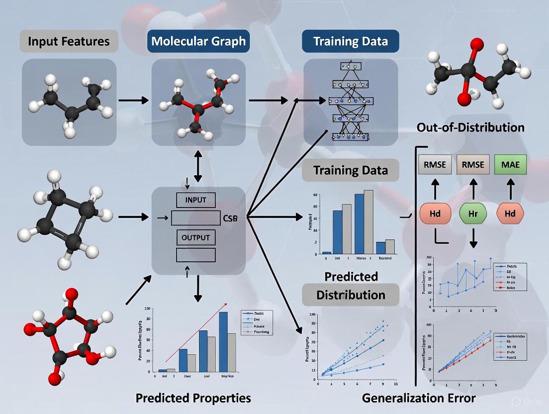
The discovery of new, high-performing materials and molecules fundamentally depends on identifying candidates with property values that fall outside the bounds of known data. However, machine learning (ML) models, which are increasingly central to accelerating discovery, often struggle with out-of-distribution (OOD) generalization, where they must make accurate predictions for these novel candidates. This challenge is acute in molecular property prediction (MPP), where a model's failure to extrapolate can lead to missed opportunities in drug and material design [1] [7]. The core of the problem lies in the complex entanglement of molecular functional groups. This often leads to inconsistent semantics, where molecules sharing what appear to be identical invariant substructures can exhibit drastically different properties, severely confusing ML models [33].
To address this, Consistent Semantic Representation Learning (CSRL) has emerged as a powerful multi-view framework. CSRL enhances OOD molecular property prediction by ensuring that the semantic information—the underlying meaning related to a molecule's function or property—is consistently represented across different molecular data views. By exploring the potential correlation between consistent semantic information and molecular properties in a dedicated semantic space, CSRL provides a robust solution to the distribution shifts that plague traditional models [33].
This technical support center is designed to help researchers, scientists, and drug development professionals successfully implement and troubleshoot the CSRL framework in their own experiments, ultimately advancing their work in dealing with OOD generalization.
Key Concepts: CSRL Framework and Components
The CSRL framework is designed to learn molecular representations that remain consistent and reliable even when the model encounters data outside its training distribution. Its architecture primarily consists of two key modules [33]:
- Semantic Uni-Code (SUC) Module: This module addresses the problem of inconsistent mapping of semantic information in different molecular representation forms (e.g., molecular graph vs. fingerprint). It works by adjusting incorrect embeddings into the correct, unified embeddings for these different forms.
- Consistent Semantic Extractor (CSE) Module: This module uses non-semantic information as training labels to guide a discriminator's learning process. This helps suppress the model's reliance on non-semantic, or "spurious," information that may be present in the different molecular representation embeddings, forcing it to focus on the consistent, core semantics.
The Scientist's Toolkit: Essential Components for a CSRL Experiment
Table 1: Key research reagents and computational tools for implementing CSRL.
| Item Name | Type | Primary Function in CSRL |
|---|---|---|
| Molecular Graphs | Data Representation | Provides a structured view of the molecule (atoms as nodes, bonds as edges) for model input [34]. |
| SMILES Strings | Data Representation | A text-based line notation offering a sequential, string-based view of the molecular structure. |
| RDKit | Software Library | Used to generate molecular descriptors and convert SMILES strings into featured molecular graphs [34]. |
| Semantic Uni-Code (SUC) | Algorithmic Module | Corrects embedding inconsistencies between different molecular representations (e.g., graph vs. SMILES) [33]. |
| Consistent Semantic Extractor (CSE) | Algorithmic Module | Extracts the core, invariant semantics by suppressing reliance on non-semantic information in the embeddings [33]. |
| Graph Neural Network (GNN) | Model Architecture | A common backbone for learning from the graph-based view of a molecule [34]. |
Diagram 1: High-level workflow of the CSRL framework.
Frequently Asked Questions (FAQs)
Q1: What is "inconsistent semantics" in the context of molecular property prediction, and why is it a problem for OOD generalization?
Inconsistent semantics occurs when molecules that share identical invariant substructures, as identified by a model, exhibit drastically different properties. This is often due to the complex entanglement of molecular functional groups and the presence of "activity cliffs." This inconsistency confounds models that try to learn simple structure-property relationships. For OOD generalization, where a model encounters entirely new molecular scaffolds or property ranges, this problem is magnified, leading to highly inaccurate predictions. The CSRL framework directly addresses this by learning to map different molecular representations to a unified semantic space where this inconsistency is minimized [33].
Q2: My model performs well on the validation set (in-distribution) but fails to identify true high-performing candidates during screening. How can CSRL help?
This is a classic symptom of poor OOD extrapolation. Traditional models are often trained to minimize error on data from the same distribution, which does not guarantee performance on the extreme, high-value tails of the property distribution. CSRL is explicitly designed for this scenario. By learning consistent semantic representations that are invariant to distribution shifts, it improves extrapolative precision—the fraction of true high-performing candidates correctly identified. For example, one OOD property prediction method improved precision by 1.8x for materials and 1.5x for molecules, and boosted the recall of high-performing candidates by up to 3x [1].
Q3: What are the most common molecular "views" used in a multi-view framework like CSRL?
The multi-view approach leverages different representations of the same molecular object. The most common views are:
- Molecular Graph View: The molecule is represented as a graph with atoms as nodes and bonds as edges, often with features for atoms (e.g., degree, formal charge) and bonds (e.g., conjugation, stereo configuration) [34].
- SMILES String View: The Simplified Molecular Input Line Entry System (SMILES) provides a text-based, sequential representation of the molecule [34]. Other views can include molecular fingerprints (like Morgan fingerprints) or 3D conformers, providing complementary information for the model to learn a more comprehensive representation.
Q4: Are there any publicly available benchmarks to evaluate my CSRL model's OOD performance?
Yes, the community is developing standardized benchmarks for this purpose. A prominent example is BOOM (Benchmarking Out-Of-distribution Molecular property predictions). BOOM evaluates over 140 model and task combinations on 10 diverse molecular property datasets, providing a robust framework for assessing OOD generalization. Using such benchmarks is crucial for meaningful comparisons and progress in the field [7].
Troubleshooting Guides
Issue 1: Poor OOD Performance Despite High In-Distribution Accuracy
Problem: Your CSRL model achieves low mean absolute error (MAE) on the validation set (which is from the same distribution as the training data) but performs poorly on the OOD test set, failing to identify molecules with extreme property values.
Solution:
- Verify Your Data Splitting Strategy: Ensure your training and test splits are based on the property value distribution, not a random split. The OOD test set should consist of samples from the tail ends of the property distribution. A common method is to use a kernel density estimator to select the molecules with the lowest probability scores (e.g., the lowest 10%) for the OOD set [7] [1].
- Inspect the SUC Module: The Semantic Uni-Code module is responsible for aligning embeddings from different views. Check its output to ensure that similar molecules from different views (e.g., graph and SMILES) are indeed being mapped to similar points in the unified semantic space. If alignment is poor, review the training objective and loss function of this module.
- Strengthen the CSE Module: The Consistent Semantic Extractor must effectively suppress non-semantic information. If OOD performance is weak, consider adjusting the training signal (the non-semantic labels) used to guide the discriminator to ensure it is effectively forcing the model to ignore spurious correlations [33].
Issue 2: Model Fails to Learn Meaningful Unified Representations
Problem: The learned unified representation H does not show a promising structure and performs poorly on downstream tasks like clustering or classification.
Solution:
- Review the Degradation Learning Strategy: In frameworks like SCMRL (a semantically consistent multi-view method), an initialized unified representation
His degenerated back to the view-specific spaces. This strategy dynamically balances the weights of different views. If this process is failing, the integration of multi-view information will be suboptimal. Check the reconstruction loss for each view [35]. - Check the Contrastive Learning Alignment: The contrastive learning strategy is meant to align the semantic labels of both view-specific representations and the unified representation. Ensure that the contrastive loss is effectively minimizing the distance between positive pairs (different views of the same molecule with consistent semantics) and maximizing it for negative pairs [35] [36].
- Validate Input Features: For the molecular graph view, ensure that the atom and bond features (e.g., atom type, degree, hybridization; bond type, conjugation) are correctly calculated and encoded. Using a library like RDKit can help standardize this process [34].
Issue 3: Unstable Training or Slow Convergence
Problem: During the training of the CSRL model, the loss values fluctuate wildly or decrease very slowly.
Solution:
- Adjust Learning Rates for Different Modules: The SUC and CSE modules may have different optimal learning rates. Consider using a smaller learning rate for the pre-trained components (if any) and a larger one for newly initialized modules.
- Monitor Intermediate Outputs: Use visualization tools (like t-SNE or UMAP) to periodically check the embeddings produced by the SUC module throughout training. This can help you identify if the model is collapsing or failing to learn meaningful patterns early on.
- Confirm Batch Statistics: When using the relative distance between samples within a batch to enhance regression performance (a technique mentioned in some contrastive learning methods), ensure that the batch size is sufficient and that the distance metric is appropriate for your data [34].
Experimental Protocols & Performance Data
Standardized OOD Evaluation Protocol
To fairly evaluate any CSRL model, follow this standardized protocol derived from recent benchmarks [7] [1]:
- Dataset Selection: Use established molecular property datasets such as those from QM9 (e.g., HOMO-LUMO gap, dipole moment) or MoleculeNet (e.g., ESOL, FreeSolv).
- OOD Splitting: For a given property, fit a Kernel Density Estimator (KDE) to the property value distribution. Assign the molecules with the lowest probability density (e.g., the bottom 10%) to the OOD test set. The remaining molecules are randomly split into training and in-distribution (ID) validation sets.
- Evaluation Metrics: Report standard metrics like Mean Absolute Error (MAE) separately for the ID and OOD sets. Crucially, also report extrapolative precision and recall for the top-k% of high-performing candidates in the OOD set.
Reported Performance of Semantic Consistency Methods
Table 2: Performance improvements from consistent semantic representation learning.
| Model / Framework | Key Approach | Reported Improvement | Evaluation Context |
|---|---|---|---|
| CSRL Framework [33] | Semantic Uni-Code & Consistent Semantic Extractor | Average ROC-AUC improved by 6.43% vs. 11 state-of-the-art models. | OOD Molecular Property Prediction on 12 datasets. |
| Bilinear Transduction [1] | Reparameterizes prediction based on differences between materials. | 1.8x better extrapolative precision for materials; 1.5x for molecules; 3x boost in recall of top candidates. | OOD Property Prediction for solids and molecules. |
| FMGCL [34] | Graph contrastive learning with partial feature masking. | Outperformed state-of-the-art methods on 12 benchmarks from MoleculeNet and ChEMBL. | Molecular Property Prediction (MPP). |
Diagram 2: Workflow for creating OOD evaluation splits.
Frequently Asked Questions (FAQs)
FAQ 1: What is the primary goal of invariant representation learning in molecular science? The primary goal is to identify causal substructures within molecules that are invariantly predictive of a target property across different environments or distribution shifts. This approach enhances the generalization capability of machine learning models, ensuring they make accurate predictions on out-of-distribution (OOD) data, which is crucial for real-world drug discovery and material design [37] [38].
FAQ 2: Why do models that perform well on in-distribution (IID) data often fail on OOD data? Models often fail because they learn to rely on spurious correlations from non-causal, environmental substructures in the training data. When these correlations change in the test environment, the model's performance deteriorates. This is compounded by activity cliffs, where molecules with similar structures can have drastically different properties, and the complex entanglement of functional groups within molecules [37].
FAQ 3: What are "inconsistent semantics" and how do they affect OOD generalization? Inconsistent semantics occur when the same molecular substructure (e.g., a hydroxy group) is mapped to different property information (e.g., hydrophilicity or hydrophobicity) depending on its molecular context. This inconsistency misleads models that try to identify invariant substructures from a single representation form (like a molecular graph alone), harming their OOD performance [37].
FAQ 4: What is the role of "environment modeling" in improving OOD generalization? Traditional methods focus solely on isolating invariant subgraphs. Modern approaches argue that environmental substructures (the non-invariant parts) are not merely noise; they can interact with and influence the causal rationales. Explicitly modeling and generating diverse environments helps the model learn to discount spurious correlations and leverage potential environment-invariance interactions for more robust predictions [38] [39].
FAQ 5: According to recent benchmarks, how well do current models perform on OOD tasks? The BOOM benchmark, evaluating over 150 model-task combinations, indicates that no existing model achieves strong OOD generalization across all tasks. Even the top-performing models exhibited an average OOD error that was three times larger than their in-distribution error. This highlights that OOD generalization remains a significant frontier challenge in chemical machine learning [7] [40].
Troubleshooting Guides
Problem 1: Poor OOD Generalization Despite High ID Accuracy
Symptoms:
- Model performance drops significantly on data from new structural classes or experimental settings.
- The model fails to identify true high-performing candidates during virtual screening.
Possible Causes and Solutions:
| Cause | Solution |
|---|---|
| Reliance on Spurious Features: The model is leveraging non-causal, environmentally-specific substructures for prediction. | Implement invariant learning frameworks like DIR [38] or IRM-based methods [39] that enforce the model to predict based on substructures whose causal relationship with the label is stable across different environments. |
| Limited Environment Diversity: The training data lacks sufficient diversity in environmental (spurious) substructures. | Use a knowledge-enhanced graph growth generator [38] [39] to artificially expand the training set with diverse environmental patterns, forcing the model to focus on more fundamental invariants. |
| Inconsistent Semantic Mapping: The model misinterprets the meaning of a substructure due to a lack of contextual information. | Adopt a consistent semantic representation learning (CSRL) framework [37]. This uses multiple molecular representations (e.g., graphs and fingerprints) to align and extract unified semantic information, ensuring consistent interpretation of substructures. |
Problem 2: Failure to Capture Complex Property-Substructure Relationships
Symptoms:
- Model predictions are insensitive to small but critical structural changes (activity cliffs).
- Extracted invariant subgraphs are insufficient to explain the property label.
Possible Causes and Solutions:
| Cause | Solution |
|---|---|
| Ignoring Environment-Invariance Interactions: The property is not fully determined by an isolated invariant subgraph but is influenced by its interaction with the environment. | Move beyond hard subgraph extraction. Implement a soft causal interaction module [38] [39] that uses cross-attention to allow dynamic information exchange between the identified invariant rationale and its environmental context. |
| Insufficient Molecular Representation: Using only a single form of molecular representation (e.g., only the graph) fails to capture all relevant chemical semantics. | Fuse multiple molecular representations. For example, the CSRL framework [37] jointly learns from molecular graphs and molecular fingerprints to construct a more robust, unified semantic representation. |
Problem 3: Low Recall for High-Performing OOD Candidates
Symptoms:
- During virtual screening, the model misses a large number of true high-value candidates that have property values outside the training distribution.
Possible Causes and Solutions:
| Cause | Solution |
|---|---|
| Inadequate Extrapolation in Output Space: Standard regression models struggle to predict property values outside the range seen during training. | Employ a transductive prediction method like Bilinear Transduction (MatEx) [1]. Instead of predicting a property from a material directly, it learns to predict the property difference between two materials based on their representational difference, enabling better extrapolation. |
| Overly Conservative Predictions: The model is not "confident" enough when predicting in uncharted regions of the property space. | Leverage methods specifically designed for OOD extrapolative precision. Bilinear Transduction has been shown to boost the recall of high-performing OOD candidates by up to 3x compared to standard baselines like Ridge Regression or CrabNet [1]. |
Experimental Protocols
Protocol 1: Implementing a Consistent Semantic Representation Learning (CSRL) Framework
This protocol is based on the CSRL framework designed to extract consistent semantics from different molecular representations to improve OOD generalization [37].
1. Objective: To learn molecular representations that capture consistent, invariant semantics across different molecular forms (graph and fingerprint) to enhance OOD prediction performance.
2. Materials/Reagents:
| Material/Software | Function |
|---|---|
| Molecular Graphs | Primary input data structure representing atoms (nodes) and bonds (edges). |
| Molecular Fingerprints (e.g., ECFP, Morgan) | Binary vector representation of molecular features, serving as a complementary input form. |
| Graph Neural Network (GNN) | Encodes the molecular graph into a latent embedding. |
| Fingerprint Encoder (e.g., MLP) | Encodes the molecular fingerprint into a latent embedding. |
| SUC Module | Semantic Uni-Code module: A contrastive learning module that aligns graph and fingerprint embeddings into a unified semantic space. |
| CSE Module | Consistent Semantic Extractor: An adversarial training module that discriminates and extracts the consistent semantics while suppressing non-semantic information. |
3. Workflow Diagram: CSRL Framework
4. Step-by-Step Procedure:
- Step 1: Input Encoding. Pass a molecular graph through a GNN and its corresponding molecular fingerprint through a separate encoder (e.g., an MLP) to obtain their respective initial embeddings.
- Step 2: Semantic Unification (SUC Module). Use a contrastive learning objective to adjust the graph and fingerprint embeddings. The goal is to pull the embeddings of the same molecule closer in the semantic space while pushing away embeddings of different molecules, ensuring different representation forms of the same entity convey the same core information.
- Step 3: Consistent Semantic Extraction (CSE Module). Feed the aligned embeddings into an adversarial discriminator. This module uses a consistent semantic loss function (e.g., based on entropy) to force the extraction of information that is consistent between the graph and fingerprint embeddings, actively suppressing non-semantic or inconsistent information.
- Step 4: Property Prediction. The final unified semantic representation is used for the downstream molecular property prediction task.
- Step 5: Evaluation. Benchmark the model on OOD datasets, such as those in the DrugOOD or ADMEOOD benchmarks, using metrics like ROC-AUC. CSRL has been shown to improve the average ROC-AUC by 6.43% over 11 state-of-the-art models [37].
Protocol 2: Evaluating OOD Generalization with the BOOM Benchmark
This protocol outlines how to use the BOOM benchmark to systematically evaluate a model's OOD performance [7] [40].
1. Objective: To rigorously assess the out-of-distribution generalization capability of molecular property prediction models across a wide range of tasks and dataset splits.
2. Materials/Reagents:
| Material/Software | Function |
|---|---|
| BOOM Benchmark Suite | A collection of chemically-informed OOD tasks for molecular property prediction. |
| Model to be Evaluated | Any deep learning model for molecular property prediction (e.g., GNNs, chemical foundation models). |
| OOD Splits | Dataset splits designed to test generalization, such as splitting by molecular scaffolds or property value ranges. |
3. Workflow Diagram: BOOM Evaluation
4. Step-by-Step Procedure:
- Step 1: Model Training. Train the model on the provided in-distribution (ID) training set for a specific property prediction task.
- Step 2: In-Distribution Evaluation. Evaluate the trained model on an ID test set, which shares the same data distribution as the training set. Record standard metrics like Mean Absolute Error (MAE) or ROC-AUC.
- Step 3: Out-of-Distribution Evaluation. Evaluate the same model on the OOD test sets provided by BOOM. These sets are constructed to be distributionally shifted from the training data (e.g., different molecular scaffolds).
- Step 4: Performance Gap Analysis. Compare the model's performance on the ID and OOD sets. A significant performance drop (e.g., OOD error being 3x larger than ID error, as commonly found) indicates poor OOD generalization [7] [40].
- Step 5: Ablation Studies. Use BOOM's framework to perform ablations, investigating how factors like model architecture, molecular representation, pre-training strategies, and hyperparameter optimization impact OOD performance.
Table 1: OOD Performance of Various Frameworks on Molecular and Materials Datasets
| Framework / Model | Key Approach | Performance Highlights |
|---|---|---|
| Bilinear Transduction (MatEx) [1] | Transductive, predicts property differences. | Improved extrapolative precision by 1.5x for molecules; Boosted recall of top OOD candidates by up to 3x. |
| Consistent Semantic Representation Learning (CSRL) [37] | Aligns semantics from graphs and fingerprints. | Improved average ROC-AUC by 6.43% vs. 11 SOTA models on 12 OOD datasets. |
| Soft Causal Learning (CauEMO) [38] [39] | Models environment-invariance interactions. | Demonstrated superior generalization on 7 datasets (DrugOOD, synthetic Motif) vs. invariant-only baselines. |
| BOOM Benchmark Top Performer [7] [40] | (Benchmark Result) | Average OOD error was 3x larger than In-Distribution (ID) error, indicating a significant generalization challenge. |
| Invariant Rationale Models (e.g., DIR) [38] | Discovers invariant causal subgraphs. | Can fail when environmental patterns expand or when properties complexly depend on environment-invariance interactions. |
Diagnosing Failure Points and Implementing Performance Optimization Strategies
FAQs on Systematic Biases in Molecular Property Prediction
1. What are systematic biases in molecular property prediction, and why are they problematic? Systematic biases are consistent, non-random errors that skew model predictions in specific directions. In molecular property prediction, a major bias is prebleaching in single-molecule photobleaching (smPB) experiments, which systematically underestimates oligomer sizes by missing fluorescent subunits bleached before data recording begins [41]. Such biases are problematic because they make models unreliable for real-world applications, especially when dealing with new, out-of-distribution (OOD) data, leading to incorrect conclusions in critical areas like drug discovery [41] [42].
2. How does out-of-distribution (OOD) data relate to systematic bias? OOD data refers to data that significantly differs from the model's training distribution. Traditional models assume training and test data are identically distributed; when this assumption fails (a distribution shift), systematic prediction errors often occur [43]. For example, a model trained primarily on one class of molecules may be systematically biased against another class not well-represented in the training set, degrading performance on clinically relevant but OOD compounds [42] [43].
3. What are the main types of distribution shift that can cause biases? The formalization of distribution shifts identifies three main types [43]:
- Covariate Shift: The input data distribution
P(X)changes between training and test data, but the conditional distributionP(Y|X)remains the same. - Label Shift: The output label distribution
P(Y)changes, but the underlying relationshipP(X|Y)remains consistent. - Concept Shift: The fundamental relationship between inputs and outputs
P(Y|X)changes over time or across domains.
4. What experimental methods can correct for systematic biases like prebleaching? A key method involves using chemically constructed multimeric standards of known stoichiometry (e.g., dimers, trimers) [41]. By comparing the known distribution of these standards to the distribution measured by your experiment, you can estimate the bias parameter (e.g., prebleaching probability, B). This parameter then constrains and corrects the data obtained from your heterogeneous, unknown samples, turning an ill-posed problem into a solvable one [41].
5. What computational strategies can improve generalization and correct for biases?
- Transfer Learning: Leveraging knowledge from a data-rich source task to improve performance on a data-poor target task, often through pre-training and fine-tuning [43].
- Advanced Contrastive Learning: Frameworks like MolFCL incorporate chemical prior knowledge (e.g., molecular fragment reactions) during pre-training to learn more robust molecular representations that are less susceptible to biases from irrelevant structural variations [44].
- Functional Group Prompting: Integrating knowledge of functional groups—substructures critical to molecular properties—during model fine-tuning to guide predictions and provide interpretability [44].
Troubleshooting Guides
Issue 1: Model Performance Degrades on New, Unseen Molecular Scaffolds
Problem: Your model, which performed well on its training data, shows significantly worse accuracy when predicting properties for molecules with different core scaffolds (an OOD problem) [42].
Solution: Implement Scaffold-Based Splitting and OOD Generalization Techniques
- 1. Diagnose: Use the "Scaffold Split" method to evaluate your model. Split your dataset so that molecules in the training and test sets have different molecular scaffolds. A large performance drop between random splits and scaffold splits indicates poor OOD generalization [42] [44].
- 2. Apply Remediation:
- Utilize Transfer Learning: Pre-train your model on a large, diverse, unlabeled molecular dataset (e.g., from ZINC15) to learn general chemical representations. Then, fine-tune it on your specific, smaller, labeled dataset [43] [44].
- Employ Robust Models: Use models specifically designed for OOD learning, such as those incorporating domain adaptation or generalization techniques that aim to learn features invariant to domain shifts [43].
Issue 2: Correcting for Systematic Experimental Bias in Oligomer Stoichiometry
Problem: In single-molecule photobleaching (smPB) experiments, your raw data appears dominated by monomers, but you suspect prebleaching is causing you to miss larger oligomers [41].
Solution: Quantitative Correction Using Multimeric Standards
- 1. Experimental Design:
- Synthesize Standards: Chemically synthesize covalent multimeric standards (e.g., bis- and tris-rhodamine-labeled peptides) where the true oligomeric state is known [41].
- Acquire Data: Perform smPB experiments on these standard samples under identical conditions to your unknown samples.
- 2. Data Analysis and Correction:
- Estimate Bias Parameter (B): Fit the prebleaching probability B by comparing the measured photobleaching step distribution of the standards to their known, true distribution. The fit is guided by binomial statistics, as each fluorophore has a probability B of being bleached before measurement [41].
- Apply the Correction: Use the derived B parameter as a constraint to correct the raw distribution obtained from your unknown sample (e.g., IAPP oligomers). This will yield a bias-corrected estimate of the true oligomeric distribution [41].
The following workflow outlines this experimental correction protocol:
Issue 3: Poor Model Performance on Scarce or Imbalanced Molecular Property Data
Problem: Limited or imlabeled data for a specific property (e.g., low aqueous solubility) leads to poor model performance and an inability to generalize.
Solution: Leverage Self-Supervised Learning and Data Augmentation
- 1. Self-Supervised Learning (SSL):
- Pre-training: Use an SSL framework like MolCLR or MolFCL to pre-train a model on a large corpus of unlabeled molecules (millions of compounds). The model learns general chemical representations by solving pretext tasks, such as predicting masked atoms or contrasting differently augmented views of the same molecule [44].
- Fine-tuning: Subsequently, fine-tune the pre-trained model on your smaller, labeled dataset for the specific property of interest. This transfers the general knowledge to your specialized task [43] [44].
- 2. Chemically-Aware Data Augmentation: When generating augmented views of a molecule for contrastive learning, use methods that preserve chemical validity. The MolFCL framework uses fragment-based augmentations that leverage BRICS decomposition, which respects reaction chemistry and does not destroy the original molecular environment, leading to more meaningful learning [44].
Experimental Protocols & Data
Quantitative Impact of Prebleaching Bias
The table below summarizes how different levels of prebleaching probability (B) can skew the apparent abundance of oligomers in smPB data, based on binomial statistics [41].
| Prebleaching Probability (B) | Impact on Apparent Oligomer Distribution | Interpretation & Recommendation |
|---|---|---|
| B = 0.1 | Moderate skew. Apparent monomer abundance is inflated, but larger oligomers are still detectable. | Inference becomes less reliable. Correction is recommended [41]. |
| B = 0.2 | Severe skew. A sample truly dominated by dimers can appear monomer-dominated. | Major misinterpretation is likely. Quantitative correction is required [41]. |
| B > 0.2 | Critical skew. Larger oligomers are massively under-represented or absent in the data. | Raw data is highly unreliable. No reliable inference should be drawn without correction [41]. |
Comparative Performance of Bias-Aware Models
The following table compares the performance of various models on molecular property prediction benchmarks, highlighting the advantage of methods designed to handle distribution shifts and data scarcity. Data is based on results from MoleculeNet and TDC benchmarks [44].
| Model / Representation | Core Strategy for Robustness | Average Performance (ROC-AUC) | Key Advantage |
|---|---|---|---|
| Traditional ECFP Fingerprint | Fixed, expert-curated representation | Baseline | Simple, fast, less prone to overfitting on small data [42]. |
| Basic GNN | Learns from molecular graph structure | Varies by dataset | End-to-end learning without manual feature engineering [42]. |
| MolCLR | Self-supervised contrastive learning | Improved over basic GNN | Mitigates data scarcity via unlabeled pre-training [44]. |
| MolFCL (State-of-the-Art) | Fragment-based contrastive learning + functional group prompts | Outperforms baselines on 23/23 datasets [44] | Integrates chemical knowledge; better OOD generalization via meaningful augmentations [44]. |
Detailed Protocol: Correcting smPB Data with Standards
Objective: To quantitatively estimate and correct for prebleaching bias in single-molecule photobleaching experiments [41].
Materials:
- Rhodamine-labeled IAPP or protein of interest [41].
- Synthesized bis- and tris-rhodamine-labeled peptide standards (e.g., H2N-QK(Rh)TTK(Rh)I-CONH2 and H(Rh)N-QK(Rh)TTK(Rh)I-CONH2) [41].
- Total Internal Reflection Fluorescence (TIRF) Microscope with a 543 nm laser, high NA objective (e.g., 100×, NA 1.49), and appropriate emission filters (e.g., 605/55 nm) [41].
- Sample Slides: Cleaned glass coverslips with spin-coated 0.25% polyvinyl alcohol (PVA) film for immobilization [41].
Procedure:
- Sample Preparation:
- Dilute the standard peptides (bis and tris) and the unknown IAPP oligomer sample to a concentration of 0.5–2 nM in pH 7.5 PBS.
- Mix each sample with 0.25% PVA solution.
- Spin-coat the mixtures onto separate pre-cleaned glass coverslips and allow to dry [41].
- Data Acquisition:
- For each sample (standards and unknown), acquire time-lapse images of individual fluorescent spots using TIRF microscopy.
- Ensure the laser power and acquisition time are identical for all samples to maintain consistent conditions.
- Record until all fluorophores in a spot are bleached [41].
- Data Analysis:
- For each fluorescent spot, count the number of discrete photobleaching steps.
- Build a step-size distribution histogram for each standard sample and the unknown sample.
- Bias Correction:
- Let θ be the true proportion of an n-mer in the standard sample. The measured proportion of a k-mer (where k ≤ n) arising from an n-mer follows binomial statistics:
P(k|n) = C(n,k) * (1-B)^k * B^(n-k). - Use the known true distribution of the standards (e.g., 100% dimer or trimer) and the measured distribution to solve for the prebleaching probability B.
- Validate B by ensuring it consistently corrects both the dimer and trimer standard data to their known values.
- Apply this B parameter to the raw distribution from the unknown IAPP sample to reconstruct the true, bias-corrected oligomeric distribution [41].
- Let θ be the true proportion of an n-mer in the standard sample. The measured proportion of a k-mer (where k ≤ n) arising from an n-mer follows binomial statistics:
The Scientist's Toolkit: Research Reagent Solutions
| Reagent / Material | Function in Experiment |
|---|---|
| Bis-/Tris-Rhodamine Peptide Standards | Covalently linked multimers of known stoichiometry; serve as internal controls to quantify systematic prebleaching bias [41]. |
| Rhodamine (TAMRA) Fluorophore | A fluorescent marker chemically linked to peptides; its photobleaching steps are counted to determine stoichiometry [41]. |
| Polyvinyl Alcohol (PVA) Film | A hydrophilic polymer used to immobilize and disperse individual oligomers on a coverslip for single-molecule imaging [41]. |
| ZINC15 Database | A large, publicly available database of commercially available compounds; used as a source of millions of unlabeled molecules for self-supervised pre-training of models [44]. |
| Therapeutics Data Commons (TDC) | A collection of datasets for various therapeutic development tasks; used for benchmarking model performance across diverse molecular properties [44]. |
| Extended-Connectivity Fingerprints (ECFP) | A circular fingerprint that encodes molecular substructures; a traditional fixed representation resilient to data scarcity [42]. |
| BRICS Algorithm | A method for decomposing molecules into logical fragments based on chemical rules; used in MolFCL to create chemically meaningful augmented views for contrastive learning [44]. |
Methodologies for Robust Molecular Property Prediction
The following diagram illustrates a robust molecular property prediction pipeline that integrates self-supervised learning and functional group knowledge to combat bias and improve OOD generalization, as exemplified by the MolFCL framework [44].
In molecular property prediction, the "Scaling Law Paradox" describes the phenomenon where machine learning models achieve diminishing returns on Out-of-Distribution (OOD) performance despite being trained with increasing amounts of data and parameters [45]. This presents a critical challenge for drug discovery and materials science, where accurately predicting properties for novel, previously unseen molecular structures is essential for innovation [10] [14]. While models excel on in-distribution (ID) data, performance often degrades significantly on OOD data, with one large-scale benchmark reporting an average OOD error three times larger than ID error [10] [46]. This technical support center provides troubleshooting guidance for researchers grappling with these challenges.
The Scientist's Toolkit: Research Reagent Solutions
Table 1: Essential solutions and resources for OOD molecular property prediction research.
| Item | Primary Function | Utility in OOD Research |
|---|---|---|
| BOOM Benchmark [10] [46] | Standardized OOD performance evaluation | Provides 10 molecular property datasets with tailored OOD splits to systematically test model generalization beyond training distribution. |
| ACS (Adaptive Checkpointing with Specialization) [47] | Multi-task learning (MTL) training scheme | Mitigates negative transfer in MTL by checkpointing optimal model parameters for each task, enabling accurate predictions with as few as 29 labeled samples. |
| Fourier Feature Mapping [48] | Input representation technique | Helps models learn periodic patterns and high-frequency functions by transforming raw inputs, potentially improving extrapolation to unseen data ranges. |
| Therapeutic Data Commons (TDC) [14] | Curated molecular data repository | Offers pre-processed ADMET and bioactivity prediction datasets for benchmarking model performance on various OOD splitting strategies. |
| Pre-trained Molecular Models [49] | Foundation for transfer learning | Provides robust structural feature extractors; can be fused with knowledge from LLMs to create more generalizable molecular representations. |
Frequently Asked Questions & Troubleshooting Guides
FAQ 1: Why does my model's performance degrade on novel molecular scaffolds, and how can I improve it?
Answer: Performance degradation occurs because models often learn shortcuts from the training data distribution and fail to capture the underlying physical principles that generalize to new chemical spaces [50]. This is a manifestation of OOD brittleness.
Troubleshooting Guide:
- Action: Implement stricter data splitting.
- Protocol: Instead of random splits, use scaffold-based splits or, for a greater challenge, chemical similarity clustering (e.g., UMAP-based clustering using ECFP4 fingerprints) to generate your OOD test sets [14]. This more accurately simulates real-world discovery scenarios where novel scaffolds are targeted.
- Action: Integrate external knowledge.
- Protocol: Augment your model's inputs by leveraging Large Language Models (LLMs). Prompt LLMs like GPT-4o or DeepSeek to generate knowledge-based features and executable code for molecular vectorization, then fuse these features with structural representations from a graph neural network [49].
- Action: Adopt a multi-task learning scheme with safeguards.
- Protocol: Use the Adaptive Checkpointing with Specialization (ACS) method. Train a shared GNN backbone with task-specific heads. During training, independently checkpoint the best model parameters for each task when its validation loss reaches a new minimum, protecting tasks from detrimental parameter updates from other tasks [47].
FAQ 2: I am using multi-task learning, but some tasks are hurting others' performance. What is happening?
Answer: You are likely experiencing Negative Transfer (NT), where gradient conflicts or imbalances between tasks cause shared model updates that are detrimental to one or more tasks [47]. This is especially common with imbalanced training datasets.
Troubleshooting Guide:
- Action: Diagnose task imbalance.
- Protocol: Quantify task imbalance using the formula ( Ii = 1 - \frac{Li}{\max Lj} ), where ( Li ) is the number of labeled entries for task ( i ) [47]. A higher ( I_i ) indicates a more severe data scarcity for that task.
- Action: Implement ACS or similar methods.
- Protocol: As described in FAQ 1, ACS is specifically designed to mitigate NT. Compared to standard MTL, it preserves the benefits of shared representations while using task-specific checkpointing to prevent performance degradation [47].
- Action: Explore data augmentation.
- Protocol: Systematically incorporate additional molecular property data, even from sparse or weakly related tasks, to act as a form of augmentation during multi-task training. This can help stabilize the learning of the shared backbone [51].
FAQ 3: The scaling laws suggest my model should keep improving, but OOD performance is plateauing. Is scaling the solution?
Answer: This is the core of the Scaling Law Paradox. Scaling models (more data, parameters, compute) often leads to logarithmic or power-law returns for OOD generalization, requiring exponentially more resources for linear accuracy gains [45]. A model with strong inductive biases is frequently more effective than a generic, larger model.
Troubleshooting Guide:
- Action: Prioritize inductive bias over pure scale.
- Protocol: For specific molecular properties, choose architectures with high inductive bias. For instance, use E(3)-invariant or equivariant GNNs (e.g., IGNN, EGNN) which build physical symmetries directly into the model, often leading to better OOD generalization than larger but less constrained transformer models [10].
- Action: Analyze the scaling relationship.
- Protocol: When evaluating the effect of model scale, plot your accuracy metric against computational cost (FLOPs) or model parameters on a log-log scale. Be aware that a straight line on a log-log plot actually represents a power-law relationship with potentially severe diminishing returns, where required compute can scale as the 20th power of desired accuracy [45].
- Action: Use model ensembles.
- Protocol: Instead of training a single massive model, train several smaller models of intermediate size and average their predictions. This can yield better OOD generalization for a given computational budget [52].
Experimental Protocols for OOD Benchmarking
Protocol 1: Creating a Property-Based OOD Split
This protocol outlines a robust method for generating OOD test sets based on molecular property values, as used in the BOOM benchmark [10].
Diagram 1: Workflow for property-based OOD splitting.
Detailed Steps:
- Dataset Preparation: Start with a curated molecular property dataset (e.g., from QM9 or TDC) containing molecular structures (as SMILES or graphs) and numerical property values [10] [14].
- Density Estimation: Fit a Kernel Density Estimator (KDE) with a Gaussian kernel to the distribution of the target property values for all molecules in the dataset.
- Probability Scoring: Use the fitted KDE to obtain a probability score for each molecule based on its property value. Molecules at the tail ends of the distribution will have the lowest probabilities.
- Split Creation: Select the molecules with the lowest KDE probability scores (e.g., the lowest 10%) to form the OOD test set. This captures molecules with atypical, extreme property values.
- ID Set Creation: Randomly sample molecules from the remaining, higher-probability pool to create the in-distribution (ID) test set. The leftover molecules are used for training and validation [10].
Protocol 2: Evaluating ID vs. OOD Performance Correlation
This protocol assesses whether good in-distribution performance reliably predicts good OOD performance, a key assumption often proven false [14].
Diagram 2: Protocol for evaluating ID and OOD performance correlation.
Detailed Steps:
- Model Training: Train a diverse set of models (e.g., Random Forest, various GNNs, pre-trained GNNs) on your prepared training set [14].
- ID Evaluation: Calculate a performance metric (e.g., ROC-AUC, RMSE) for each model on the ID test set.
- OOD Evaluation: Calculate the same performance metric for each model on the OOD test set. It is critical to perform this evaluation on different types of OOD splits (e.g., scaffold, chemical cluster, property-based) [14].
- Correlation Analysis: For each OOD splitting method, compute the Pearson correlation coefficient (r) between the models' ID performance and their OOD performance.
- Interpretation:
- A strong positive correlation (e.g., r ~ 0.9 for scaffold splits) suggests that selecting the best ID model may also yield the best OOD model for that particular split type.
- A weak correlation (e.g., r ~ 0.4 for cluster-based splits) indicates that ID performance is a poor proxy for OOD generalization, necessitating direct OOD benchmarking for model selection [14].
Disclaimer: The solutions and protocols provided here are based on current research. The field of OOD generalization is evolving rapidly, and we encourage you to validate these approaches against your specific datasets and problem domains.
Data Generation and Curation Strategies for Enhanced Generalization
Frequently Asked Questions
1. Why does my model, trained on benchmark data, perform poorly on my proprietary compounds? This is a classic Out-of-Distribution (OOD) problem. Your proprietary compounds likely occupy a different region of chemical space than your training data. The model has learned the distribution of the benchmark data but fails to generalize to your novel structures. This is particularly common with "dark proteins" where you have limited known binders [53]. To diagnose, use tools like AssayInspector to compare the chemical feature distributions (e.g., using ECFP4 fingerprints or RDKit descriptors) between your benchmark and proprietary datasets [54].
2. How can I improve model performance when I have very little experimental data for my target property? Multi-task learning (MTL) is a highly effective strategy for this low-data regime. By training a single model to predict multiple related molecular properties simultaneously, the model learns more robust and generalized representations. A Graph Neural Network (GNN) can be trained to predict your primary target alongside auxiliary properties (even sparse or weakly related ones), which acts as a form of data augmentation and can significantly enhance prediction quality [51].
3. I am integrating public datasets to increase my training data size, but my model performance is getting worse. What is happening? This is often caused by dataset misalignments and annotation inconsistencies. Differences in experimental protocols, measurement conditions, and chemical space coverage between public sources introduce noise into the integrated dataset. Naive aggregation can degrade performance. Before integration, perform a rigorous Data Consistency Assessment (DCA) using tools like AssayInspector to identify outliers, batch effects, and significant distributional shifts between the sources [54].
4. What is the difference between Covariate Shift and Concept Shift in my molecular property predictions? Understanding the type of distribution shift is key to selecting the right solution:
- Covariate Shift: Occurs when the distribution of input molecules (
P(X)) changes between training and test data, but the fundamental relationship between the molecule and its property (P(Y|X)) remains constant. An example is training on simple drug-like molecules and testing on complex natural products [43]. - Concept Shift: Occurs when the relationship between the molecule and its property (
P(Y|X)) itself changes. For instance, the same molecule could have different solubility measurements under different experimental conditions (e.g., pH, temperature) [43]. Techniques like Transfer Learning can help address covariate shift, while concept shift may require more sophisticated domain adaptation methods.
5. How can I check the consistency of my aggregated dataset before model training? The AssayInspector tool provides a systematic framework for this. It generates a report that alerts you to several critical issues [54]:
- Dissimilar Datasets: Datasets with significantly different chemical descriptor profiles.
- Conflicting Datasets: Datasets that provide differing property annotations for shared molecules.
- Divergent Datasets: Datasets with low molecular overlap.
- Redundant Datasets: Datasets with a very high proportion of shared molecules. The tool also performs statistical tests, like the Kolmogorov-Smirnov test for regression tasks, to flag datasets with significantly different endpoint distributions [54].
Troubleshooting Guides
Issue: Poor OOD Generalization on Novel Chemical Scaffolds
Problem: A model trained on the QM9 dataset performs accurately on test molecules from QM9 but fails to generalize to new, synthetically designed compounds with different scaffolds.
Diagnosis: This is a covariate shift problem. The model is facing molecules with a feature distribution (P(X)) that differs from its training data.
Solution Steps:
- Characterize the Shift: Use chemical space visualization (e.g., UMAP projection based on ECFP4 fingerprints) to compare the training (QM9) and test (novel compounds) distributions. This will visually confirm the distributional misalignment [54].
- Apply Transfer Learning: Pre-train a Graph Neural Network on a large, diverse auxiliary dataset (e.g., ChEMBL) to learn general chemical representations. Then, fine-tune the model on your specific QM9 data. This approach has been shown to improve the ROC-AUC for molecular property prediction by an average of 7.2% by providing a better starting point for the model [43].
- Implement Multi-Task Learning: If you have data for other molecular properties, even from different sources, frame the problem as multi-task. Train a single GNN to predict multiple properties, which encourages the model to learn features that are general and transferable, rather than specific to the narrow QM9 distribution [51].
Troubleshooting workflow for covariate shift
Issue: Performance Degradation After Integrating Public Datasets
Problem: After combining several public ADME datasets (e.g., from TDC and Obach et al.) to train a half-life prediction model, the model's accuracy is worse than when trained on a single, consistent source.
Diagnosis: The integrated dataset contains distributional misalignments and annotation inconsistencies due to differences in experimental conditions and data curation practices.
Solution Steps:
- Run a Data Consistency Assessment (DCA): Use the AssayInspector package on your aggregated data.
- Input: Your combined dataset with source labels.
- Let the tool compute summary statistics, similarity matrices, and perform statistical tests (KS-test) [54].
- Review the Insight Report: Analyze the generated alerts. The report will highlight:
- Which specific source datasets have significantly different endpoint distributions (e.g., half-life values from Obach et al. vs. TDC) [54].
- The presence of conflicting annotations for molecules that appear in multiple sources.
- Outliers and out-of-range data points that may be skewing the model [54].
- Clean and Stratify: Based on the report:
- Remove or correct conflicting data points after manual validation.
- Consider stratified sampling or weighting schemes during training to balance the influence of different data sources, rather than simply merging them.
- If discrepancies are too large, train a model on the most reliable gold-standard source (e.g., Obach et al. for half-life) and use the others for auxiliary pre-training [54].
Workflow for resolving data integration issues
The Scientist's Toolkit: Key Research Reagents & Solutions
The following table details essential computational tools and data resources for tackling OOD generalization in molecular property prediction.
| Item Name | Function / Purpose | Key Specification |
|---|---|---|
| AssayInspector [54] | Python package for Data Consistency Assessment (DCA) prior to model training. Identifies dataset misalignments, outliers, and batch effects. | Generates statistical reports (KS-test, Chi-square), similarity matrices, and UMAP visualizations. |
| Graph Neural Networks (GNNs) [51] | Deep learning architecture for multi-task molecular property prediction. Learns from molecular graph structure. | Effective for data augmentation in low-data regimes by sharing representations across prediction tasks. |
| Therapeutic Data Commons (TDC) [54] | Provides standardized benchmark datasets for molecular property prediction, including ADME properties. | Contains curated datasets but may have distributional misalignments with gold-standard sources. |
| Transfer Learning [43] | A method to pre-train a model on a large, diverse source dataset (e.g., ChEMBL) and fine-tune it on a specific, smaller target task. | Reported to increase ROC-AUC by an average of 7.2% for molecular property prediction tasks [43]. |
| QM9 Dataset [51] | A public benchmark dataset containing quantum-mechanical properties for small organic molecules. | Used in controlled experiments to study the effects of multi-task learning and data augmentation. |
Experimental Protocols
Protocol 1: Systematic Data Consistency Assessment with AssayInspector
Purpose: To systematically identify and characterize inconsistencies across multiple molecular property datasets before integration to ensure robust model training.
Methodology:
- Input Preparation: Compile all datasets (e.g., from TDC, Obach et al., Lombardo et al.) into a unified format. Ensure each data point is tagged with its source [54].
- Tool Execution: Run the AssayInspector package. The tool will automatically:
- Compute Summary Statistics: Generate a table of descriptive parameters (mean, standard deviation, min, max, quartiles) for the target property per dataset [54].
- Perform Statistical Testing: Apply the two-sample Kolmogorov-Smirnov (KS) test for regression tasks to compare property distributions between every pair of datasets. A low p-value indicates a significant difference [54].
- Analyze Chemical Space: Calculate molecular similarities (Tanimoto coefficient on ECFP4 fingerprints) within and between datasets. Generate a UMAP projection to visualize the coverage and overlap of different datasets in chemical space [54].
- Identify Conflicts: Flag molecules that appear in multiple sources but have conflicting property annotations [54].
- Report Generation: Review the insight report from AssayInspector, which contains alerts for dissimilar, conflicting, divergent, and redundant datasets [54].
Protocol 2: Multi-Task Learning for Low-Data Regimes
Purpose: To enhance the prediction accuracy of a target molecular property for which only scarce data is available by jointly learning related auxiliary tasks.
Methodology:
- Data Curation: Select your primary target property dataset (e.g., a small in-house dataset of fuel ignition properties). Gather auxiliary datasets for other molecular properties (e.g., solubility, logP, metabolic stability) even if they are from different sources or are partially incomplete [51].
- Model Architecture: Construct a Multi-task Graph Neural Network (MT-GNN). The typical architecture includes:
- A shared GNN backbone that processes the molecular graph and generates a common latent representation for each molecule.
- Multiple task-specific prediction heads (usually fully connected layers) that take the shared representation as input and predict individual properties [51].
- Model Training: Train the entire model jointly. The loss function is a weighted sum of the losses for each individual task (e.g., Mean Squared Error for regression tasks). This setup forces the shared backbone to learn features that are generally useful across multiple properties, which regularizes the model and improves generalization on the primary, low-data task [51].
- Controlled Evaluation: Compare the performance of the multi-task model against a single-task model trained only on the primary target property. The evaluation should be performed on a held-out test set for the primary property to quantify the improvement gained from data augmentation via multi-task learning [51].
Multi-task GNN architecture for data augmentation
Hyperparameter Optimization Approaches Tailored for OOD Scenarios
Frequently Asked Questions (FAQs)
General Concepts
Q1: What is Out-of-Distribution (OOD) Generalization and why is it critical in molecular property prediction?
OOD generalization refers to a model's ability to maintain performance when test data comes from a different distribution than the training data. In molecular property prediction, this is crucial because discovering new high-performance materials and molecules requires identifying extremes with property values outside the known distribution [1]. Models often struggle with true extrapolation, and their performance can significantly degrade on OOD data, which is a key challenge in reliable drug discovery and materials informatics [7] [3].
Q2: How does hyperparameter optimization for OOD scenarios differ from standard practices?
Standard hyperparameter optimization typically aims to maximize performance on a validation set from the same distribution as the training data. In contrast, OOD-focused hyperparameter optimization uses a small OOD validation set to guide the search for hyperparameters that ensure robustness to distribution shifts [55]. The search space is also often expanded to include coefficients for various robust losses and regularizers, providing more granular control over the adaptation process [55].
Technical Implementation
Q3: What are the most effective hyperparameter optimization methods for OOD generalization?
Bayesian Optimization has emerged as a powerful solution for OOD scenarios, as it builds a probabilistic model of the objective function and sequentially refines it, typically requiring fewer evaluations than grid or random search [56] [57]. For fine-tuning foundation models, methods like AutoFT demonstrate that optimizing hyperparameters—including loss coefficients—on a small OOD validation set significantly improves generalization to unseen distributions [55].
Q4: Which hyperparameters are most impactful for OOD performance in molecular property prediction?
Key hyperparameters include those controlling model capacity, optimization (like learning rate), and regularization. For specific optimizers like Adam, the learning rate, beta1, and beta2 are critical [57]. Research also highlights the importance of dynamic batch size strategies in conjunction with Bayesian optimization for optimal OOD performance on molecular properties [56].
Troubleshooting Common Experimental Issues
Q5: My model performs well in-distribution but poorly on OOD data, even after hyperparameter optimization. What should I investigate?
First, verify that your OOD validation set is truly representative of meaningful distribution shifts, such as novel chemical spaces or structural symmetries not seen during training [3]. Ensure your hyperparameter search space is sufficiently expressive, including weight coefficients for different robust losses [55]. Also, analyze the representation space to confirm that your OOD test data genuinely lies outside the training domain, as many heuristic OOD splits may still be within the interpolation regime [3].
Q6: How can I reliably benchmark the OOD performance of my molecular property prediction model?
Utilize established benchmarks like BOOM (Benchmarking Out-Of-distribution Molecular property predictions), which provides a standardized framework for evaluating over 140 combinations of models and property prediction tasks [7]. Ensure your evaluation includes diverse types of distribution shifts, such as leave-one-element-out or leave-one-structural-group-out tasks, to thoroughly assess generalization [3].
Q7: I have limited OOD data available for validation. Can I still optimize for robustness?
Yes, approaches like AutoFT have demonstrated success with small OOD validation sets (up to 1000 labeled examples) from a single unseen distribution to optimize hyperparameters for improved generalization across multiple unseen test distributions [55]. The key is leveraging this data specifically for hyperparameter optimization rather than direct model training.
Troubleshooting Guides
Issue 1: Poor OOD Generalization Despite Extensive ID Hyperparameter Tuning
Symptoms:
- High accuracy on validation data drawn from the same distribution as training data.
- Significant performance drop on data with novel chemical elements, structural symmetries, or property value ranges.
Diagnostic Steps:
- Audit your validation data: Confirm your validation set for hyperparameter optimization contains representative OOD samples. Relying solely on an ID validation set will not select for robust hyperparameters [55].
- Check your hyperparameter search space: Ensure it includes parameters specifically relevant to robustness, such as coefficients for regularization terms that penalize over-reliance on spurious correlations [55].
- Quantify the distribution shift: Use tools like kernel density estimation on the representation space to verify that your OOD test set is genuinely distant from your training data. Many tasks perceived as OOD may actually be interpolation [3].
Solutions:
- Adopt an OOD-aware optimization protocol: Implement a method like AutoFT, which uses a small OOD validation set to directly optimize fine-tuning hyperparameters [55].
- Expand the hyperparameter space: Include weight coefficients for different loss functions and robust regularizers to give the optimization algorithm more control over the trade-off between ID fit and OOD robustness [55].
- Incorporate advanced optimization methods: Use Bayesian Optimization to efficiently navigate the complex hyperparameter landscape for OOD performance, as it requires fewer expensive evaluations [56] [57].
Issue 2: Inconsistent OOD Performance Across Different Types of Distribution Shifts
Symptoms:
- Model generalizes well to some OOD tasks (e.g., new chemical elements) but fails on others (e.g., new structural groups).
- Performance degradation is unpredictable and varies greatly across benchmarks.
Diagnostic Steps:
- Benchmark comprehensively: Use a diverse set of OOD tasks, such as those provided by the BOOM benchmark, to identify the specific types of shifts your model struggles with [7].
- Analyze failure modes: Investigate whether poor performance is linked to compositional (chemical) or structural (geometric) differences between training and test sets. SHAP analysis can help identify the source of prediction errors [3].
- Evaluate model calibration: Check if the model is overconfident in its incorrect OOD predictions, which is a common issue.
Solutions:
- Employ model selection based on worst-case performance: Consider using Distributionally Robust Optimization (DRO) principles during hyperparameter selection to improve performance under the worst-case distribution [58].
- Explore transductive methods: For property value extrapolation, methods like Bilinear Transduction, which learns how properties change as a function of material differences, can improve OOD precision [1].
- Regularize to preserve pre-trained features: When fine-tuning foundation models, use hyperparameter optimization to find the right strength for regularization techniques (e.g., L2 penalty on weight updates) that prevent the model from distorting useful pre-trained representations [55].
Experimental Protocols & Data
Protocol 1: Bayesian Optimization for OOD Molecular Property Prediction
This protocol is adapted from research on optimizing convolutional neural networks for molecular properties [56].
1. Objective: Identify hyperparameters for a deep learning model that minimize prediction error on out-of-distribution molecular data. 2. Model Setup:
- Use a fully convolutional sequence-to-sequence (ConvS2S) model as the base architecture.
- Represent molecules as SMILES strings or molecular graphs. 3. Hyperparameter Search Space:
- Dynamic Batch Size: Incorporate a strategy for adjusting batch size based on SMILES enumeration ratios.
- Core Hyperparameters: Learning rate, weight decay, number of layers, hidden layer dimensions, dropout rate.
- Feature Learning: Include hyperparameters controlling the integration of additional chemical features from a feedforward network. 4. Optimization Procedure:
- Method: Bayesian Optimization.
- Validation Set: Use a dedicated validation set containing molecules from a distribution different from the training set.
- Iterations: Run for a predetermined number of trials (e.g., 50-100), each training a model with a new hyperparameter set and evaluating on the OOD validation set.
- Selection Criterion: Choose the hyperparameter set that achieves the best performance on the OOD validation set.
BO Workflow for OOD: This diagram illustrates the iterative process of using Bayesian Optimization to find hyperparameters that maximize performance on an OOD validation set.
Protocol 2: AutoFT for Robust Fine-Tuning of Foundation Models
This protocol is based on the AutoFT method for fine-tuning models to preserve OOD robustness [55].
1. Objective: Fine-tune a pre-trained foundation model on a task-specific dataset without degrading its performance on out-of-distribution data. 2. Prerequisites:
- A pre-trained foundation model (e.g., a model trained on a large corpus of molecular data).
- A small labeled validation set (up to 1000 samples) from an OOD distribution. This should not be the final test distribution. 3. Hyperparameter Search Space:
- Standard Parameters: Learning rate, weight decay.
- Loss Coefficients: Weight coefficients for multiple loss components (e.g., task-specific loss, feature distillation loss, L2 regularization toward the pre-trained weights). 4. Optimization Procedure:
- Method: Perform hyperparameter optimization (e.g., using Bayesian Optimization or random search) to maximize performance on the small OOD validation set.
- Fine-Tuning: For each hyperparameter candidate, fine-tune the foundation model on the task-specific training data using the combined loss function.
- Output: The final fine-tuned model produced by the best-found hyperparameters.
Performance Data
The following tables summarize key quantitative findings from recent research on OOD generalization and hyperparameter optimization.
Table 1: OOD Performance of Molecular Property Prediction Models (BOOM Benchmark)
| Model Category | Example Models | Average OOD Error vs. ID | Key Finding |
|---|---|---|---|
| Deep Learning Models | Various GNNs, CNNs | Up to 3x larger | No model achieved strong OOD generalization across all tasks [7]. |
| Models with High Inductive Bias | Specific GNN architectures | Lower for simple properties | Can perform well on OOD tasks with simple, specific properties [7]. |
| Chemical Foundation Models | LLM-Prop, others | Still large | Current models do not show strong OOD extrapolation capabilities [7]. |
Table 2: Impact of Robust Fine-Tuning (AutoFT) on OOD Performance
| Benchmark/Dataset | Previous SOTA Performance | AutoFT Performance | Improvement |
|---|---|---|---|
| WILDS-iWildCam | (Previous best) | New SOTA | +6.0% [55] |
| WILDS-FMoW | (Previous best) | New SOTA | +1.5% [55] |
| Generalization | Across 9 natural distribution shifts | Consistently improved | Outperformed existing robust fine-tuning methods [55]. |
Table 3: OOD Generalization in Leave-One-Element-Out Tasks (Materials Science)
| Model | % of Tasks with R² > 0.95 | Poor Performance Elements | Primary Cause of Poor Performance |
|---|---|---|---|
| ALIGNN (GNN) | 85% | H, F, O | Compositional (Chemical) Differences [3] |
| XGBoost (Tree) | 68% | H, F, O | Compositional (Chemical) Differences [3] |
The Scientist's Toolkit: Key Research Reagents & Solutions
Table 4: Essential Components for OOD Hyperparameter Optimization Experiments
| Item | Function in the Context of OOD Generalization |
|---|---|
| OOD Validation Set | A small set of labeled data from a distribution different from the training data. It is used as the target for hyperparameter optimization to directly select for robustness [55]. |
| Bayesian Optimization Framework | A software library (e.g., Ax, Optuna) that facilitates the efficient search of hyperparameter spaces by building a probabilistic model of performance, reducing the number of required model trainings [56] [57]. |
| Pre-trained Foundation Model | A model (e.g., a large GNN or transformer) trained on vast and diverse molecular datasets. It serves as a rich prior, and its robust features must be preserved during task-specific fine-tuning [55] [59]. |
| Benchmark Suite (e.g., BOOM) | A standardized collection of OOD tasks and datasets, such as the BOOM benchmark, which allows for systematic evaluation and comparison of model robustness [7]. |
| Representation Space Analysis Tool | Methods like Kernel Density Estimation (KDE) or PCA to visualize and quantify the distance between training and test data, helping to diagnose if a task is truly OOD [3] [1]. |
Frequently Asked Questions
FAQ 1: What are molecular descriptors and why are they fundamental to QSAR modeling? Molecular descriptors are numerical representations of a molecule's structural and physicochemical characteristics. They serve as the input variables for Quantitative Structure-Activity Relationship (QSAR) models, which correlate these chemical features with biological or pharmaceutical activity. The selection of optimal descriptors is crucial for building predictive and interpretable models that can assist in lead molecule selection, reducing the reliance on expensive and time-consuming high-throughput screening [60].
FAQ 2: My model performs well on known chemical space but fails on novel compounds. What is the cause? This is a classic challenge of Out-of-Distribution (OOD) generalization. Models often struggle to predict property values that fall outside the range of the training data distribution. This is particularly critical in materials and molecule discovery, where the goal is to find high-performance extremes. Even top-performing models can exhibit an average OOD error three times larger than their in-distribution error, highlighting the need for specialized approaches to OOD extrapolation [1] [7].
FAQ 3: How do traditional molecular descriptors differ from modern, AI-driven representations?
- Traditional Descriptors rely on explicit, rule-based feature extraction. This includes:
- Molecular Descriptors: Quantify physical/chemical properties (e.g., molecular weight, log P) or are calculated from the molecular graph (e.g., topological indices like the Wiener index) [60] [61].
- Molecular Fingerprints: Encode substructural information as binary strings or numerical vectors (e.g., Extended-Connectivity Fingerprints - ECFP) [61].
- Modern AI-Driven Representations use deep learning to learn continuous, high-dimensional feature embeddings directly from data. These include graph neural networks (GNNs) that operate on the molecular graph and language models that process string-based representations like SMILES [61]. These methods can capture more complex structure-property relationships.
FAQ 4: When should I use feature selection methods, and which ones are recommended? Descriptor selection is recommended to reduce computation time, improve model interpretability, and mitigate the risk of overfitting from noisy or redundant descriptors [60]. The table below summarizes common selection methods:
| Method Category | Example | Brief Explanation | Advantages/Disadvantages |
|---|---|---|---|
| Wrapper Methods | Hybrid-Genetic Algorithm | Uses a genetic algorithm to search for a descriptor subset that optimizes a model's performance. | Can find high-performing subsets, but is computationally intensive [60]. |
| Filter Methods | Correlation-based | Selects descriptors based on their statistical correlation with the target property. | Computationally efficient, but ignores descriptor interactions [60]. |
| Embedded Methods | LASSO (L1 Regularization) | Incorporates feature selection into the model training process itself by penalizing less important descriptors. | More efficient than wrappers; built-in selection [60]. |
| Evolutionary Algorithms | Evolutionary Multipattern Fingerprint (EvoMPF) | Generates interpretable, dataset-specific fingerprints by evolving structural queries. | Offers intrinsic interpretability and requires minimal parameter tuning [62]. |
FAQ 5: What are some advanced strategies for improving OOD property prediction? Recent research has proposed novel methods to address OOD extrapolation. One such approach is Bilinear Transduction, a transductive method that reparameterizes the prediction problem. Instead of predicting a property value directly from a new material, it learns how property values change as a function of the difference in representation between a known training example and the new sample. This has been shown to improve extrapolative precision for materials by 1.8x and boost the recall of high-performing candidates by up to 3x [1].
Troubleshooting Guides
Issue 1: Model Overfitting and Poor Generalization to New Data
- Symptoms: Excellent performance on the training set but poor accuracy on the validation/test set, especially for compounds with property values outside the training range.
- Potential Causes & Solutions:
| Cause | Diagnostic Check | Solution and Experimental Protocol |
|---|---|---|
| Too many redundant/noisy descriptors | Check the correlation matrix of descriptors. A high number of pairwise correlations indicates redundancy. | Protocol: Apply Feature Selection. 1. Split your data into training, validation, and (if possible) a held-out OOD test set. 2. Standardize the descriptor values. 3. Apply a feature selection method (see FAQ 4). For example, use LASSO regression. 4. Train your model using only the selected descriptors. 5. Validate on the OOD test set to confirm improved generalization [60]. |
| Inadequate representation for the task | The model fails to capture the structural nuances relevant to the target property. | Protocol: Evaluate Advanced Representations. 1. Benchmark traditional fingerprints (e.g., ECFP) against modern graph-based representations (e.g., from a Graph Neural Network). 2. Use a consistent model architecture (e.g., Random Forest) for the benchmark. 3. Evaluate performance specifically on an OOD test set where property values exceed the training maximum or minimum [61] [7]. |
| Training data lacks diversity | The chemical space of the test set is not well-represented in the training set. | Protocol: Implement a Transductive Learning Strategy. 1. Adapt a method like Bilinear Transduction [1]. 2. During inference, for a new candidate molecule, select a known training example. 3. Predict the new property value based on the training example's value and the learned relationship between their representation difference and property difference. |
Issue 2: Inability to Extrapolate to High-Value Property Ranges
- Symptoms: The model accurately predicts values within the training distribution but consistently underestimates (or overestimates) high-value extremes, leading to low recall of top candidates.
- Potential Causes & Solutions:
| Cause | Diagnostic Check | Solution and Experimental Protocol |
|---|---|---|
| Standard regression loss functions | The model is penalized equally for all errors, not prioritizing accuracy on high-value extremes. | Protocol: Reframe as an Extrapolative Precision Task. 1. Define a high-value threshold (e.g., top 30% of property values). 2. Instead of purely minimizing MAE, evaluate models based on "extrapolative precision"—the fraction of true top candidates correctly identified among the model's top predictions on an OOD test set [1]. 3. Optimize model selection and hyperparameters to maximize this metric. |
| Model architecture with low inductive bias | Highly flexible models may interpolate well but fail to learn the underlying physical principles needed for extrapolation. | Protocol: Leverage Models with High Inductive Bias. 1. For tasks with simple, specific properties, models with strong built-in constraints (high inductive bias) can perform better OOD. 2. Systematic benchmarking, as in the BOOM study, has shown that no single model is best for all OOD tasks. It is essential to test multiple architectures on your specific OOD benchmark [7]. |
Experimental Protocols
Protocol 1: Benchmarking Molecular Representations for OOD Generalization
Objective: To systematically evaluate the performance of different molecular representations on predicting properties for out-of-distribution compounds.
Data Curation and Splitting:
- Select a dataset with molecular structures and a target property.
- Split the data into training, validation, and test sets. To create an OOD test set, split based on property value ranges (e.g., the top 30% of values are held out as the OOD test set, while the lower 70% constitute the in-distribution training and validation sets) [1].
Representation Generation:
- Generate multiple representations for all molecules:
- Traditional: ECF4/6 fingerprints, a set of topological and physicochemical descriptors.
- Modern: Graph embeddings from a pre-trained GNN, SMILES-based embeddings from a transformer model.
- Generate multiple representations for all molecules:
Model Training and Evaluation:
- Train identical model architectures (e.g., Ridge Regression, Random Forest) on the training set using each representation type.
- Tune hyperparameters on the in-distribution validation set.
- Evaluate final models on the held-out OOD test set. Key metrics should include Mean Absolute Error (MAE) and Extrapolative Precision/Recall [1].
Protocol 2: Evolutionary Algorithm for Interpretable Fingerprint Generation
Objective: To generate a tailored, interpretable molecular representation for a specific dataset and prediction task using the EvoMPF framework [62].
Algorithm Setup:
- Input your dataset of molecular structures (as SMILES strings) and the target property.
- The evolutionary algorithm requires no initial parameter tuning for most applications.
Fingerprint Evolution:
- The algorithm initializes a population of structural queries based on common chemical patterns.
- It iteratively applies evolutionary operations (mutation, crossover) to these queries.
- Fitness is evaluated by the predictive performance of a model using the fingerprint generated by these queries.
Model Building and Interpretation:
- Use the evolved fingerprint (EvoMPF) to train your final predictive model.
- Leverage the intrinsic interpretability of the EvoMPF. The structural queries that make up the fingerprint are directly inspectable (e.g., using the SMARTS language), allowing you to identify which molecular substructures were most important for the prediction [62].
The Scientist's Toolkit: Research Reagent Solutions
| Item | Function in Analysis |
|---|---|
| Extended-Connectivity Fingerprints (ECFP) | A circular fingerprint that captures atomic environments and is widely used for similarity searching and QSAR modeling [61]. |
| Topological Descriptors (e.g., Wiener Index) | Graph-invariant descriptors calculated from the molecular structure that capture molecular branching, size, and shape [60]. |
| SMILES (Simplified Molecular-Input Line-Entry System) | A string-based representation that provides a compact and human-readable encoding of a molecule's structure, serving as input for language models [61]. |
| Graph Neural Networks (GNNs) | A deep learning architecture that operates directly on the molecular graph, learning representations by passing messages between atoms and bonds [61]. |
| Bilinear Transduction Framework | A transductive learning method designed to improve zero-shot extrapolation to out-of-distribution property values [1]. |
| Evolutionary Multipattern Fingerprint (EvoMPF) | An evolutionary algorithm that generates a dataset-specific, interpretable molecular fingerprint for machine learning applications [62]. |
Workflow and Relationship Diagrams
Diagram 1: Molecular Descriptor Selection and OOD Validation Workflow
Diagram 2: Transductive OOD Prediction via Bilinear Model
Rigorous Benchmarking and Comparative Analysis of OOD Methodologies
FAQs and Troubleshooting Guide
This technical support center provides practical guidance for researchers working with the BOOM (Benchmarking Out-Of-distribution Molecular property predictions) benchmark, addressing common challenges in molecular property prediction and out-of-distribution (OOD) generalization [7] [10].
What is the core objective of the BOOM benchmark?
The BOOM benchmark is designed to systematically evaluate the out-of-distribution generalization capabilities of machine learning models for molecular property prediction. It addresses a critical gap in model assessment, as molecule discovery inherently requires accurate predictions on data that falls outside the training distribution [10].
Why does my model perform well in-distribution but fail on BOOM's OOD test splits?
This is an expected finding. BOOM's evaluation revealed that even top-performing models exhibited an average OOD error three times larger than their in-distribution error [7] [10]. This performance drop is due to models struggling to extrapolate to the tail ends of molecular property distributions, which is the explicit focus of the BOOM OOD split methodology [10].
Which model architecture should I choose for OOD molecular property prediction?
No single model currently achieves strong OOD generalization across all tasks [10]. However, BOOM's extensive evaluation of over 140 model-task combinations offers these insights [7] [10]:
- Deep learning models with high inductive bias can perform well on OOD tasks involving simple, specific properties.
- Current chemical foundation models (like MolFormer and ChemBERTa), while promising, do not yet show strong OOD extrapolation capabilities.
- The benchmark establishes OOD property prediction as a "frontier challenge," indicating that model selection should be guided by your specific property of interest and the results published in the BOOM benchmark study.
How is the OOD test set constructed in BOOM?
BOOM defines OOD with respect to model outputs (property values), not inputs [10]. The methodology is as follows:
- For a given molecular property dataset, a Kernel Density Estimator (with a Gaussian kernel) is fitted to the distribution of property values [10].
- The OOD test set comprises molecules with the lowest 10% of probability scores as determined by the KDE. This selects molecules at the tail ends of the property value distribution, simulating the discovery of novel molecules with extreme properties [10].
My model's performance is highly variable across different OOD tasks. Is this normal?
Yes. Model performance is highly task-dependent. A model that excels at predicting one property OOD (e.g., isotropic polarizability) may perform poorly on another (e.g., HOMO-LUMO gap). It is essential to evaluate models across the suite of 10 properties in BOOM to understand their generalization strengths and weaknesses [10].
BOOM Benchmark at a Glance
The following table summarizes the quantitative findings from the BOOM benchmark study [10].
Table 1: Summary of BOOM Benchmark Findings
| Aspect | Details |
|---|---|
| Core Objective | Evaluate Out-Of-Distribution (OOD) generalization in molecular property prediction [10]. |
| Number of Model-Task Combinations Evaluated | More than 140 [7] [10]. |
| Key Finding on OOD Error | Average OOD error of top models was 3x larger than in-distribution error [7] [10]. |
| Number of Molecular Property Datasets | 10 (8 from QM9, 2 from the 10k Dataset) [10]. |
| OOD Split Methodology | Based on property value distribution; lowest 10% of probability scores (via KDE) form the OOD test set [10]. |
| Performance of Chemical Foundation Models | Did not show strong OOD extrapolation capabilities in current evaluations [10]. |
Experimental Protocols and Workflows
This section details the core methodologies used in the BOOM benchmark.
OOD Splitting Protocol
The workflow for creating the OOD splits, as implemented in BOOM, is as follows [10]:
Model Evaluation Framework
BOOM evaluates a diverse set of models, from traditional machine learning to advanced graph neural networks and transformers [10].
Table 2: Research Reagent Solutions - Key Models Evaluated in BOOM
| Model Name | Architecture Type | Molecular Representation | Key Characteristic |
|---|---|---|---|
| Random Forest | Traditional ML | RDKit Molecular Descriptors | Baseline model using chemically-informed features [10]. |
| ChemBERTa | Transformer | SMILES | Encoder-only model with BERT backbone, pre-trained on PubChem [10]. |
| MolFormer | Transformer | SMILES | Encoder-decoder model with T5 backbone, pre-trained on PubChem [10]. |
| Regression Transformer (RT) | Transformer | SMILES | XLNet-based model capable of masked and autoregressive generation [10]. |
| Chemprop | Graph Neural Network (GNN) | Molecular Graph (Atoms, Bonds) | Message-passing neural network for molecular property prediction [10]. |
| IGNN | Graph Neural Network (GNN) | Molecular Graph (with Pair-wise Distances) | E(3)-invariant GNN architecture [10]. |
| EGNN | Graph Neural Network (GNN) | Molecular Graph (with Atom Positions) | E(3)-equivariant GNN architecture [10]. |
| MACE | Graph Neural Network (GNN) | Molecular Graph (with Pair-wise Distances) | A state-of-the-art equivariant graph neural network [10]. |
The Scientist's Toolkit: Essential Materials
Table 3: Key Research Reagents and Datasets
| Item | Function in BOOM Context |
|---|---|
| QM9 Dataset | Source of 8 molecular properties (e.g., HOMO, LUMO, dipole moment) calculated via DFT for 133,886 small organic molecules [10]. |
| 10k Dataset | Source of 2 properties (density and solid heat of formation) for 10,206 experimentally synthesized molecules from the Cambridge Crystallographic Database [10]. |
| Kernel Density Estimator (KDE) | A non-parametric way to estimate the probability density function of a property, used to define the OOD splits [10]. |
| RDKit Featurizer | Generates a vector of 125+ chemically-informed molecular descriptors, used as input for baseline models [10]. |
| SMILES Representation | A string-based representation of molecules; the input format for transformer-based models like ChemBERTa and MolFormer [10]. |
| Molecular Graph Representation | A graph where atoms are nodes and bonds are edges; the input format for GNNs like Chemprop and EGNN [10]. |
Troubleshooting Guide & FAQs for Molecular Property Prediction
Frequently Asked Questions
Q1: My model achieves low Mean Absolute Error (MAE) on the test set, but fails to identify any top-performing candidate molecules during virtual screening. What is wrong, and which metric should I use?
A1: A low MAE does not guarantee success in identifying extreme, high-performing candidates, which is often the primary goal in discovery. You should evaluate your model using extrapolative precision and recall [1].
- Root Cause: Standard MAE measures average performance across all data points. It can be skewed by good performance on the majority of low-value compounds, masking poor performance on the rare, high-value outliers you seek.
- Solution: Implement metrics that specifically evaluate the model's ability to identify top-tier candidates. Extrapolative Precision measures the fraction of true top candidates among those your model predicts to be top candidates. Extrapolative Recall measures the fraction of all true top candidates that your model successfully identifies [1].
- Experimental Protocol:
- Define a high-performance threshold (e.g., the top 30% of property values in the entire held-out set) [1].
- Apply your trained model to an Out-of-Distribution (OOD) test set containing high-value candidates.
- From the model's predictions, select the top k candidates (e.g., the same number that meets the high-performance threshold).
- Calculate Extrapolative Precision as: (Number of true top candidates in the model's top k predictions) / (k).
- Calculate Extrapolative Recall as: (Number of true top candidates in the model's top k predictions) / (Total number of true top candidates in the test set).
Q2: How can I structure an experiment to properly test my model's ability to extrapolate to out-of-distribution (OOD) property values?
A2: Proper OOD evaluation requires carefully designed data splits that mimic real-world discovery scenarios, where you are searching for compounds with properties beyond those seen in training [1] [3].
- Root Cause: Using random train-test splits often leads to over-optimism about a model's generalizability, as the test data is statistically similar to the training data. This is often interpolation, not true extrapolation [3].
- Solution: Adopt a threshold-based data split to create a dedicated OOD test set [1].
- Experimental Protocol:
- Sort your entire dataset by the target property value.
- Training/ID Validation Set: Use all data points below a defined property value threshold for training and in-distribution (ID) validation.
- OOD Test Set: Reserve all data points above this threshold as your OOD test set. This set should contain property values outside the support of the training distribution [1].
- Train your model only on the training set and use the OOD set for final evaluation, focusing on extrapolative precision and recall.
Q3: Are there specific machine learning methods designed to improve extrapolation in molecular property prediction?
A3: Yes, classical regression models often struggle with extrapolation. Recent research has introduced methods like Bilinear Transduction and other specialized OOD techniques [1] [63].
- Root Cause: Standard models learn to predict property values directly from molecular features. When the test data has fundamentally different feature-property relationships, these models fail.
- Solution: Use models specifically designed for OOD generalization. For example, the Bilinear Transduction method reparameterizes the problem. Instead of predicting a property for a new molecule, it predicts how the property changes from a known training example based on the difference in their molecular representations [1]. This approach has been shown to improve OOD prediction accuracy by 1.5x for molecules and boost the recall of high-performing candidates by up to 3x [1].
- Implementation Workflow: The following diagram illustrates the core reasoning of the Bilinear Transduction method.
Quantitative Performance of OOD Methods
The following table summarizes the performance improvements offered by an advanced OOD method compared to baseline models on benchmark datasets for solid-state materials and molecules [1].
Table 1: Performance Improvement of Bilinear Transduction for OOD Property Prediction [1]
| Category | Metric | Improvement Factor | Notes / Baseline Comparison |
|---|---|---|---|
| Solids (Materials) | Extrapolative Precision | 1.8x | Compared to Ridge Regression, MODNet, and CrabNet on AFLOW, Matbench, and Materials Project datasets. |
| Molecules | Extrapolative Precision | 1.5x | Compared to Random Forest and MLP baselines on MoleculeNet datasets (ESOL, FreeSolv, Lipophilicity, BACE). |
| Solids & Molecules | Recall of High-Performing Candidates | Up to 3.0x | Measures the improved identification of true top-tier OOD candidates. |
The Scientist's Toolkit: Essential Research Reagents for OOD Molecular Property Prediction
Table 2: Key Resources for Building and Evaluating OOD Models
| Research Reagent / Resource | Function & Explanation | Example / Source |
|---|---|---|
| OOD Benchmark Datasets | Publicly available datasets with curated splits for testing extrapolation on molecules and materials. | MoleculeNet [1] [44], TDC (Therapeutics Data Commons) [44] [64], Matbench [1] [3] |
| Representation Learning Models | Pre-trained models that convert molecular structures (e.g., SMILES, graphs) into numerical vectors, providing a strong feature foundation. | MolCLR [44], GEM [44], CMPNN [44] |
| OOD-Generalization Algorithms | Specialized ML models designed to maintain performance under distribution shifts. | Bilinear Transduction (MatEx) [1], DEROG [63] |
| Automated Machine Learning (AutoML) Frameworks | Tools that automate the process of feature selection and model optimization, which can be leveraged to find optimal molecular representations. | MaxQsaring [64] |
| Interpretability & Explainability Tools | Methods to understand which molecular features (e.g., functional groups) the model is using for its predictions. | SHAP (SHapley Additive exPlanations) [3], Functional Group-based Prompt Learning [44] |
For researchers in molecular property prediction, the ultimate goal is to discover novel materials and compounds with exceptional characteristics—precisely those that lie outside the boundaries of known data distributions. This pursuit makes Out-of-Distribution (OOD) generalization a critical bottleneck in molecular AI. When machine learning models encounter data that significantly differs from their training distribution, performance can dramatically degrade, a phenomenon known as OOD brittleness [50]. In high-stakes fields like drug discovery, where molecular candidates with out-of-distribution properties are often the most valuable, this brittleness poses a fundamental challenge to AI-driven pipelines.
The core challenge lies in the closed-world assumption underlying most models, which presumes that test data will closely mirror the training distribution [50]. Real-world discovery processes systematically violate this assumption by seeking extremes and novelty. This analysis examines how three competing approaches—Traditional Machine Learning, Graph Neural Networks (GNNs), and Transformers—address this challenge in molecular property prediction and related domains, providing technical guidance for researchers navigating OOD generalization challenges.
Core Concepts: Defining the OOD Challenge
What Constitutes an OOD Scenario in Molecular Property Prediction?
In molecular sciences, OOD generalization can refer to two distinct but related concepts:
- Input Space Extrapolation: Generalizing to unseen classes of materials, structures, and chemical spaces (e.g., training on organic molecules and predicting inorganic crystals) [1]
- Output Space Extrapolation: Predicting property values that fall outside the range observed in training data, which is critical for discovering high-performance materials [1]
Most discovery-focused research requires output space extrapolation, as identifying extremes is fundamental to finding materials with superior properties.
Why Are Models Brittle to OOD Data?
Multiple factors contribute to OOD brittleness in molecular AI:
- Dataset Shift: Changes in data distribution between training and real-world deployment environments [50]
- High Dimensionality: The curse of dimensionality makes most of the volume in molecular descriptor spaces lie far from training data [50]
- Model Complexity: Highly parameterized models can overfit training distributions and respond unpredictably to OOD inputs [50]
- Adversarial Vulnerability: Models can be sensitive to slight molecular modifications that preserve functionality but confuse predictors [50]
- Absence of OOD Training: Supervised learning provides no guidance for handling truly novel inputs [50]
Technical Performance Comparison
Quantitative Benchmarking Across Architectures
Table 1: OOD Performance Comparison on Molecular and Materials Property Prediction
| Model Architecture | Representative Models | Avg. OOD Error Increase vs. ID | Key Strengths | Key Limitations |
|---|---|---|---|---|
| Traditional ML | Ridge Regression, Random Forest [1] | ~3x [7] | Computational efficiency, strong on simple OOD tasks with specific properties [7] | Limited capacity for complex molecular representations, struggles with structural relationships [65] |
| Graph Neural Networks | GIN, GCN, GAT [66] | ~3x [7] | Native graph representation of molecules, message-passing captures molecular topology [66] [67] | Vulnerable to graph distribution shifts, limited long-range dependency modeling [66] [68] |
| Transformers | BERT, GPT series, T5 [65] | ~3x [7] | Global attention, strong transfer learning, parallel processing [65] [69] | Extreme computational demands, data hunger, current foundation models show limited OOD extrapolation [65] [7] |
Table 2: Specialized OOD Method Performance Gains
| OOD Method | Base Architecture | Performance Improvement | Application Context |
|---|---|---|---|
| Bilinear Transduction [1] | Various | 1.8x precision for materials, 1.5x for molecules, 3x recall boost [1] | Materials and molecular property extrapolation |
| CSIB (Causal Subgraphs) [68] | GNN | Enhanced OOD robustness across shift types | Graph classification under distribution shift |
| Explainability-based Augmentation [70] | GNN | Significant OOD classification improvements | Digital pathology, graph-structured data |
| Recursive Latent Space Reasoning [69] [71] | Transformer | Improved algorithmic generalization | Compositional reasoning tasks |
The BOOM benchmark (Benchmarking Out-Of-distribution Molecular property predictions) reveals that no current architecture consistently achieves strong OOD generalization, with even top performers exhibiting average OOD errors approximately 3 times larger than in-distribution errors [7]. This underscores OOD generalization as a fundamental challenge requiring architectural innovations and specialized training paradigms.
Troubleshooting Guide: OOD Generalization Issues
Frequently Asked Questions
Q: My model achieves high in-distribution accuracy but fails to identify promising molecular candidates with out-of-distribution properties. What strategies should I prioritize?
A: Focus on methods specifically designed for output space extrapolation. The Bilinear Transduction approach has demonstrated 1.8x precision improvements for materials and 1.5x for molecules by reparameterizing the prediction problem to learn how property values change as a function of molecular differences rather than predicting absolute values [1]. This method predicts properties based on known training examples and the representation space difference between materials, enabling better extrapolation.
Q: My GNN model suffers significant performance drops when evaluating molecules from different structural classes than the training data. How can I improve cross-domain robustness?
A: Implement explainability-based graph augmentation techniques that identify and augment critical subgraphs using methods like GNNExplainer and GraphLIME [70]. This approach simulates potential OOD scenarios during training by selectively augmenting important node features based on their statistical significance and neighborhood information. Additionally, consider causal subgraph methods like CSIB that integrate invariant risk minimization with graph information bottlenecks to identify stable substructures across distributions [68].
Q: Transformer models show promising in-distribution performance but fail to extrapolate to more complex molecular reasoning tasks. Are there architectural modifications that can improve systematic generalization?
A: Recent research explores architectural enhancements including input-adaptive recurrence, algorithmic supervision, anchored latent representations via discrete bottlenecks, and explicit error-correction mechanisms [69] [71]. These modifications enable more robust algorithmic reasoning capabilities in Transformer networks, particularly for compositional tasks requiring systematic generalization beyond training distributions.
Q: How can I properly benchmark my model's OOD performance when working with limited novel molecular data?
A: Implement a rigorous evaluation protocol that clearly separates in-distribution and out-of-distribution splits based on property value thresholds, not just structural similarity [1]. Use metrics like extrapolative precision (measuring correct identification of top OOD candidates) alongside traditional MAE. The BOOM benchmark framework provides methodology for assessing performance degradation between ID and OOD settings across multiple property prediction tasks [7].
Q: What practical approaches can enhance Traditional ML models for OOD scenarios when deep learning is computationally prohibitive?
A: Leverage ensemble methods and advanced regularization techniques. Random Forests and Ridge Regression with appropriate molecular descriptors can achieve competitive performance on OOD tasks with simple, specific properties [1] [7]. Focus on feature engineering that captures chemically meaningful invariants, and consider transductive learning approaches that reformulate the prediction problem to emphasize relational patterns rather than absolute property values [1].
Experimental Protocols for OOD Generalization
Implementing Bilinear Transduction for Molecular Property Prediction
Table 3: Research Reagents for Bilinear Transduction Experiments
| Component | Function | Implementation Notes |
|---|---|---|
| Material Representations | Encodes chemical stoichiometry or molecular structure | Use Magpie composition features [1] or graph representations [7] |
| Bilinear Layer | Models property differences via representation interactions | Implement as parameterized tensor product between material pairs [1] |
| Training Triplets | Enables difference learning | Sample (A, B) pairs from training set with known property differences [1] |
| Reference-based Inference | Enables extrapolation | Predict properties relative to known training exemplars [1] |
Protocol Steps:
- Data Preparation: Split data ensuring OOD test samples have property values outside training range [1]
- Representation Learning: Convert molecular structures to appropriate feature representations (stoichiometric or graph-based)
- Triplet Sampling: During training, sample material pairs (A, B) and learn the relationship between their representation difference and property difference
- Model Training: Optimize bilinear parameters to minimize prediction error on property differences between pairs
- Reference-based Prediction: For test molecules, predict properties relative to carefully selected training exemplars
- Evaluation: Assess performance using OOD-specific metrics including extrapolative precision and recall of high-performing candidates
This approach demonstrated significant improvements in identifying high-performing molecular candidates, with 3× higher recall of OOD materials compared to conventional regression methods [1].
Explainability-Based Graph Augmentation for GNNs
Protocol Steps:
- Important Subgraph Extraction: Use GNNExplainer to identify subgraphs with maximal influence on predictions [70]
- Node Ranking: Rank nodes within important subgraphs based on their degree centrality and feature significance [70]
- Feature Importance Analysis: Apply GraphLIME to select the most crucial node features for interpretable explanations [70]
- Neighborhood-Based Augmentation: Augment important node features using features from their 1-hop neighboring nodes [70]
- Adversarial Training: Incorporate augmented samples into training to improve model robustness to distribution shifts
This method has shown significant improvements in classification performance under OOD scenarios in digital pathology, with applicability to molecular graph classification [70].
Visualization of Key Methodologies
Bilinear Transduction Workflow for Molecular Property Prediction
Explainability-Based Graph Augmentation Process
Transformer with Latent Space Reasoning for Algorithmic Generalization
The comparative analysis reveals that OOD generalization remains a significant challenge across all architectural paradigms in molecular property prediction. While specialized methods like Bilinear Transduction for traditional ML, explainability-based augmentation for GNNs, and latent space reasoning for Transformers show promising improvements, the field lacks universal solutions.
Future research directions should focus on:
- Developing better benchmarks and evaluation frameworks specifically designed for OOD scenarios in molecular sciences [7]
- Exploring hybrid architectures that combine the strengths of different approaches
- Improving foundation models' OOD extrapolation capabilities through better pre-training strategies and architectural innovations [69] [7]
- Enhancing model interpretability to better understand failure modes in OOD scenarios [70]
As molecular AI continues to evolve, addressing OOD generalization will be crucial for transforming these technologies from retrospective analysis tools into genuine discovery engines capable of identifying novel molecular candidates with exceptional properties.
FAQs: Troubleshooting Common Experimental Issues
This section addresses specific, frequently encountered challenges when working with chemical foundation models, framed within the context of out-of-distribution (OOD) generalization.
FAQ 1: My foundation model performs well on validation data but fails to generalize to novel, high-performing molecules outside its training distribution. What strategies can improve OOD extrapolation?
- Problem: This is a fundamental challenge in molecular property prediction. Models often struggle to extrapolate to property values that fall outside the range seen in the training data, which is critical for discovering high-performance materials [1].
- Solution & Protocol: Consider employing a transductive approach specifically designed for OOD property value extrapolation.
- Method: The Bilinear Transduction method (e.g., implemented in tools like MatEx) reparameterizes the prediction problem. Instead of predicting a property value for a new candidate directly, it learns how property values change as a function of material differences. Predictions are made based on a known training example and the difference in representation space between that example and the new sample [1].
- Expected Outcome: This method has been shown to improve extrapolative precision by 1.8× for materials and 1.5× for molecules, and can boost the recall of high-performing candidates by up to 3× [1].
FAQ 2: Fine-tuning a large pre-trained model on my small, specialized dataset leads to overfitting and poor performance. How can I leverage the foundation model more effectively?
- Problem: The benefits of a large pre-trained model can be lost if the fine-tuning dataset is too small and not representative of the broader task, especially for OOD tasks [7].
- Solution & Protocol: Utilize the model's latent representations for Retrieval Augmented Generation (RAG) rather than fine-tuning all parameters.
- Method: Use the pre-trained model as a fixed feature extractor. For a given query molecule, encode it into a latent representation and use this to retrieve chemically similar structures or relevant data from a knowledge base. This context is then used by a separate agent or model (like an LLM) to make predictions or design decisions [72].
- Expected Outcome: This approach facilitates structure-focused, semantic information retrieval, enabling more accurate and context-aware predictions for data-scarce tasks without the risk of overfitting from fine-tuning [72].
FAQ 3: How can I diagnose if my model's poor performance is due to a fundamental lack of transfer learning capability in the foundation model?
- Problem: It can be difficult to determine if failure is due to model architecture, data, or a lack of genuine transfer learning.
- Solution & Protocol: Conduct rigorous ablation studies on transfer learning.
- Method: Systematically hold out specific data modalities (e.g., proteins, RNA, small molecules) during pre-training and evaluate the model's performance on the held-out tasks. Compare this to models trained only on the target modality [73].
- Expected Outcome: This tests whether the model is truly learning transferable knowledge across domains. Current evidence suggests that models using unified, atom-level representations (like in some universal interatomic potentials) show more convincing transfer learning than architectures where different modalities are processed by largely separate parameters [73].
FAQ 4: My model identifies molecules with high predicted potency, but they fail in experimental validation due to toxicity or poor pharmacokinetics. How can the model account for this?
- Problem: This mirrors a major cause of failure in clinical drug development, where an over-emphasis on potency (Structure-Activity Relationship, SAR) overlooks tissue exposure and selectivity [74].
- Solution & Protocol: Move beyond simple property prediction to a Structure–Tissue exposure/selectivity–Activity Relationship (STAR) framework.
- Method: When curating training data and defining prediction tasks, include not just binding affinity or potency, but also experimental data on tissue exposure, selectivity, and pharmacokinetic properties. Train multi-task models or use multi-stage filtering to prioritize candidates with balanced profiles [74].
- Expected Outcome: This helps select drug candidates (Class I and III in the STAR framework) that have a higher likelihood of clinical success due to a better balance of efficacy, toxicity, and dose [74].
Benchmarking Performance & OOD Generalization
Understanding the current capabilities and limitations of chemical foundation models is crucial for setting realistic experimental expectations. The table below summarizes key quantitative findings from recent benchmark studies on out-of-distribution (OOD) generalization.
Table 1: Benchmarking Chemical Foundation Models on OOD Tasks
| Model / Method | Key Finding | Performance Metric | Context / Dataset |
|---|---|---|---|
| Various Deep Learning Models (140+ combinations evaluated) [7] | Poor OOD generalization is a widespread issue. No single model performs strongly across all tasks. | Average OOD error was 3x larger than in-distribution error. | BOOM benchmark for molecular property prediction. |
| Current Chemical Foundation Models [7] | Offer promising solutions for limited data but lack strong OOD extrapolation. | Did not show strong OOD generalization capabilities. | BOOM benchmark evaluation. |
| Bilinear Transduction (e.g., MatEx) [1] | Effective for property value extrapolation in virtual screening. | Improved extrapolative precision by 1.8x for materials and 1.5x for molecules; boosted recall of top candidates by up to 3x. | Evaluation on AFLOW, Matbench, and Moleculeset datasets. |
| Universal ML Interatomic Potentials (MLIPs) (e.g., UMA) [73] | A success story for transfer learning across diverse molecular systems. | Jointly trained model outperformed uni-modal baselines and previous state-of-the-art. | Trained on inorganic materials, organic molecules, and hybrid systems. |
Experimental Protocols for Assessing Capabilities
This section provides detailed, step-by-step methodologies for key experiments cited in this guide, enabling researchers to reproduce and validate critical findings.
Protocol: Evaluating OOD Property Prediction using a Transductive Approach
This protocol is based on the Bilinear Transduction method detailed in npj Computational Materials [1].
Objective: To assess a model's ability to extrapolate to higher property value ranges than those present in the training data.
Workflow:
Materials & Data:
- Datasets: Standard benchmarks such as AFLOW (computational properties), Matbench (experimental and computational properties), or MoleculeNet (molecular properties) [1].
- Data Splitting: The held-out set must be divided into an In-Distribution (ID) validation set and an Out-of-Distribution (OOD) test set, each of equal size. The OOD set should contain samples with property values outside the range of the training data [1].
Procedure:
- Model Training: Train the Bilinear Transduction model (e.g., using the open-source MatEx implementation) on the training dataset [1].
- Model Inference: For each sample in the OOD test set, make a property prediction based on a chosen training example and the difference in representation space between the two materials [1].
- Performance Evaluation:
- Calculate the Mean Absolute Error (MAE) specifically for the OOD test samples.
- Compute Extrapolative Precision: Identify the top 30% of test samples with the highest predicted property values and calculate the fraction of these that are true top OOD candidates (i.e., their actual property values are in the top 30% of the entire held-out set) [1].
Protocol: Testing Transfer Learning via Modality Hold-Out Ablation
This protocol is inspired by discussions on evaluating transfer in models like AlphaFold 3 and Universal MLIPs [73].
Objective: To determine if a multi-modal foundation model is genuinely learning transferable knowledge across different molecular domains (e.g., proteins, small molecules, materials).
Workflow:
Materials & Data:
- Model: A multi-modal foundation model architecture (e.g., transformer-based or GNN-based).
- Datasets: Large-scale datasets for each modality, such as the Protein Data Bank (PDB) for structures, the Cambridge Structural Database (CSD) for small molecules, and materials databases like the Materials Project [75] [73] [76].
Procedure:
- Model Pre-training:
- Experimental Model: Pre-train the model on a mixture of all data modalities except for one target modality (e.g., RNA).
- Control Model: Pre-train an identical model architecture only on the data from the target modality.
- Model Evaluation: Fine-tune both the experimental and control models on a downstream task-specific dataset for the held-out target modality (e.g., RNA structure prediction).
- Performance Analysis: Compare the final task performance of the two models. Genuine transfer learning is demonstrated if the model pre-trained on multiple modalities outperforms the model trained only on the target modality data [73].
This table details essential computational "reagents" – datasets, models, and benchmarks – for research in chemical foundation models and OOD generalization.
Table 2: Essential Resources for Chemical Foundation Model Research
| Resource Name | Type | Function & Application |
|---|---|---|
| BOOM Benchmark [7] | Benchmark | Systematically evaluates the Out-of-Distribution (OOD) generalization performance of molecular property prediction models across 140+ model-task combinations. |
| MatEx (Materials Extrapolation) [1] | Software Tool | An implementation of the Bilinear Transduction method for improving OOD property value extrapolation in materials and molecules. |
| Cambridge Structural Database (CSD) [75] | Dataset | A repository of experimental organic and metal-organic crystal structures. Used for pre-training foundation models like MCRT. |
| Universal Model of Atoms (UMA) [73] | Foundation Model | An example of a universal ML interatomic potential that demonstrates successful transfer learning across inorganic materials, organic molecules, and hybrid systems. |
| MCRT (Molecular Crystal Representation from Transformers) [75] | Foundation Model | A transformer-based model pre-trained on the CSD for molecular crystal property prediction, serving as a universal foundation model. |
| AFLOW, Matbench, Moleculeset [1] | Datasets | Curated collections of material and molecular properties used for benchmarking prediction tasks, especially OOD performance. |
| STAR Framework [74] | Conceptual Framework | A strategy (Structure-Tissue exposure/selectivity-Activity Relationship) for balancing drug efficacy, toxicity, and dose in candidate selection, informing model training objectives. |
The reliability of machine learning models in molecular property prediction is fundamentally constrained by the methodology used to split datasets into training and test sets. Traditional random splitting approaches often create an overly optimistic assessment of model performance by allowing information leakage between training and test distributions. This practice fails to reflect the true out-of-distribution (OOD) generalization capabilities required for real-world molecular discovery, where models must accurately predict properties for chemically distinct compounds not represented in training data. Recent systematic benchmarking reveals that even state-of-the-art models exhibit an average OOD error three times larger than their in-distribution error [10]. This performance gap underscores the critical need for advanced dataset splitting methodologies that rigorously evaluate model generalization, including kernel density estimation and similarity-based metrics that better simulate the challenges of actual molecular discovery pipelines.
Understanding the Problem: Why Traditional Data Splitting Fails
FAQ: What is information leakage and why does it inflate model performance?
Information leakage occurs when similarities between data points in the training and test sets are larger than similarities between training data and the actual data the model will encounter during real-world deployment [77]. When this happens, machine learning models can achieve excellent test performance by relying on similarity-based shortcuts that do not generalize to the intended application scenario [77]. For example, in protein-protein interaction prediction, models performing excellently on random splits often become nearly random when evaluated on protein pairs with low homology to training data [77]. This creates dangerously overoptimistic performance estimates that undermine reliable model deployment.
FAQ: How does out-of-distribution generalization relate to real-world molecular discovery?
Molecular discovery is inherently an OOD prediction problem because discovering novel molecules that extend the boundaries of known chemistry requires accurate predictions for structures that differ from the training data [10]. Success depends on the model's ability to extrapolate beyond the training distribution, either to molecules exhibiting properties beyond those of known training molecules or to structures containing new chemical substructures not previously considered [10]. Without rigorous OOD evaluation, models may appear successful in benchmarks but fail in practical discovery applications.
Novel Splitting Methodologies: Technical Approaches and Experimental Protocols
Property-Based Splitting Using Kernel Density Estimation
Experimental Protocol from BOOM Benchmark [10]
- Objective: Create OOD test sets based on molecular property values to evaluate model extrapolation capabilities.
Procedure:
- Fit a kernel density estimator (with Gaussian kernel) to the distribution of property values in the complete dataset.
- Calculate the probability of each molecule given its property value using the fitted estimator.
- Select molecules with the lowest probabilities for the OOD test split.
- For the QM9 dataset, take the lowest 10% of probability scores; for smaller datasets (e.g., 10K dataset), select a fixed number (e.g., 1000) of the lowest-probability molecules.
- Randomly sample from the remaining higher-probability molecules to create an in-distribution (ID) test set (typically 10% for QM9, 5% for 10K dataset).
- Use the remaining molecules for training and validation.
Troubleshooting Guide:
- Problem: OOD split contains too few samples for meaningful evaluation.
Solution: Adjust the percentage threshold or use absolute numbering appropriate to dataset size. Ensure OOD set is large enough for statistical significance while maintaining distribution extremity.
Problem: Kernel density estimator fails to capture multimodality in property distribution.
Solution: Use bandwidth selection techniques like cross-validation and visually inspect the fitted distribution against the data histogram.
Problem: Model performance severely degrades on OOD split.
- Solution: This indicates limited extrapolation capability. Consider architectures with stronger inductive biases or incorporating physical principles.
Similarity-Based Splitting Using Clustering Approaches
Experimental Protocol from UMAP-Based Clustering [78]
- Objective: Create challenging splits that maximize structural dissimilarity between training and test sets.
Procedure:
- Compute molecular representations (e.g., Morgan fingerprints, graph embeddings, or learned representations).
- Apply Uniform Manifold Approximation and Projection (UMAP) to reduce dimensionality while preserving both local and global structural information.
- Perform hierarchical clustering on the UMAP-reduced features to group structurally similar molecules.
- Assign entire clusters to different folds (e.g., 7 folds as used in the NCI-60 benchmark).
- Implement a leave-one-cluster-out cross-validation scheme where each fold serves as the test set once.
- For virtual screening applications, evaluate performance using early-recognition metrics (e.g., hit rate at top 100 predictions) rather than overall metrics like ROC AUC.
Troubleshooting Guide:
- Problem: UMAP produces unstable clustering across different random seeds.
Solution: Fix the UAP randomstate parameter and experiment with different mindist and n_neighbors parameters to achieve stable clustering.
Problem: Clusters have highly imbalanced sizes.
Solution: Adjust cluster resolution parameters or use balanced clustering algorithms that constrain cluster sizes.
Problem: Model performance is poor on all UMAP splits.
- Solution: This indicates limited generalization to structurally novel compounds. Consider incorporating transfer learning or domain adaptation techniques.
Combinatorial Optimization for Data Splitting
Experimental Protocol from DataSAIL [77]
- Objective: Formally define data splitting as a combinatorial optimization problem to minimize information leakage while preserving class distribution.
Procedure:
- Define the (k, R, C)-DataSAIL problem: split an R-dimensional dataset into k folds minimizing inter-fold similarity while maintaining distribution of C classes across folds.
- For one-dimensional data (single entities), ensure that similar molecules (based on defined similarity metrics) are separated between training and test sets.
- For two-dimensional data (e.g., drug-target pairs), ensure separation along both dimensions simultaneously.
- Address the NP-hard nature of the problem using a scalable heuristic based on clustering and integer linear programming (ILP).
- Implement stratification constraints to maintain similar class ratios across splits, particularly important for imbalanced datasets.
Troubleshooting Guide:
- Problem: Integer linear programming becomes computationally intensive for large datasets.
Solution: Use the clustering-based heuristic first to reduce problem size before applying ILP.
Problem: Similarity metric does not capture relevant molecular characteristics for specific property prediction task.
- Solution: Tailor similarity metrics to the target property (e.g., functional group-based similarity for toxicity prediction, topological similarity for adsorption properties).
Domain Adaptation for Realistic Material Property Prediction
Experimental Protocol from Domain Adaptation Benchmarking [79]
- Objective: Improve OOD prediction by incorporating target domain information during model training.
Procedure:
- Identify target materials of interest using domain knowledge or density-based methods.
- Generate target test sets using methods like Leave-One-Cluster-Out (LOCO) or sparse sampling in composition/property space.
- Apply domain adaptation techniques to align feature representations between source (training) and target (test) distributions.
- Implement feature-based DA (aligning feature distributions), instance-based DA (reweighting training instances), or parameter-based DA (sharing model parameters).
- Evaluate whether DA improves OOD performance compared to standard models.
Troubleshooting Guide:
- Problem: Domain adaptation fails to improve performance or degrades it.
Solution: Carefully analyze domain shift characteristics; some DA methods assume related domains and may fail with large shifts.
Problem: Limited target domain samples for adaptation.
- Solution: Use semi-supervised or few-shot domain adaptation techniques designed for low-data regimes.
Comparative Analysis: Performance Across Splitting Strategies
Table 1: Comparative Performance of Models Across Different Splitting Methodologies
| Splitting Method | Dataset | Model Type | ID Performance (MAE/R²) | OOD Performance (MAE/R²) | Performance Gap |
|---|---|---|---|---|---|
| Random Split | QM9 (HOMO-LUMO gap) | GNN | 0.08 eV (MAE) | 0.08 eV (MAE) | 0% |
| Property-Based (KDE) | QM9 (HOMO-LUMO gap) | GNN | 0.08 eV (MAE) | 0.24 eV (MAE) | 200% |
| Scaffold Split | NCI-60 | Random Forest | 0.81 (ROC AUC) | 0.79 (ROC AUC) | 2.5% |
| UMAP Clustering | NCI-60 | Random Forest | 0.81 (ROC AUC) | 0.64 (ROC AUC) | 21% |
| Random Split | Materials Project | ALIGNN | 0.03 eV (MAE) | 0.03 eV (MAE) | 0% |
| Leave-One-Element-Out | Materials Project | ALIGNN | 0.03 eV (MAE) | ~0.30 eV (MAE) | ~900% |
Table 2: Characteristics of Major Splitting Methodologies
| Methodology | Key Principle | Best-Suited Applications | Advantages | Limitations |
|---|---|---|---|---|
| Property-Based (KDE) | OOD defined by extreme property values | Discovering molecules with state-of-the-art properties | Directly aligned with discovery goals; systematic | May not capture structural novelty |
| Scaffold Split | Group by Bemis-Murcko scaffolds | Drug discovery focusing on novel chemotypes | Intuitive; ensures novel core structures | Overlooks similarity between different scaffolds |
| UMAP Clustering | Clustering in reduced-dimension space | Virtual screening of diverse compound libraries | High-quality clusters; captures global structure | Computationally intensive; parameter sensitive |
| DataSAIL Optimization | Combinatorial optimization minimizing similarity | Any scenario requiring rigorous leakage prevention | Flexible similarity definitions; theoretical foundation | Computational complexity for large datasets |
| Leave-One-Cluster-Out | Hold out entire compositional/structural clusters | Evaluating generalization to new material classes | Interpretable; physically meaningful | May overestimate if clusters are not truly novel |
Implementation Toolkit: Research Reagent Solutions
Table 3: Essential Tools and Resources for Implementing Advanced Splitting Methodologies
| Tool/Resource | Type | Functionality | Implementation Notes |
|---|---|---|---|
| DataSAIL [77] | Python package | Similarity-aware data splitting for 1D and 2D data | Supports proteins, small molecules, DNA/RNA; formulates splitting as optimization problem |
| UMAP [78] | Dimensionality reduction | Creates low-dimensional embeddings for clustering | Critical parameter: n_neighbors balances local/global structure preservation |
| RDKit [78] | Cheminformatics | Molecular fingerprinting and scaffold generation | Standard for molecular similarity calculations and structural analysis |
| Matminer [3] | Materials feature generation | Composition and structure-based descriptors | Essential for materials science applications; integrates with ML pipelines |
| Kernel Density Estimation (Scipy) | Statistical tool | Probability density estimation for property-based splitting | Bandwidth selection critically impacts OOD set definition |
| BOOM Benchmark [10] | Evaluation framework | Standardized OOD evaluation for molecular property prediction | Provides 10 molecular property datasets with predefined OOD splits |
Workflow Visualization: Implementing Rigorous Data Splitting
Data Splitting Methodology Selection Workflow
Advanced Considerations and Future Directions
FAQ: Why don't scaling laws consistently improve OOD generalization?
Contrary to traditional machine learning assumptions, increasing training set size or model complexity does not necessarily improve OOD generalization and can sometimes degrade it [3]. Analysis of representation spaces reveals that most heuristic-based OOD test data actually reside within regions well-covered by training data, meaning apparent "generalization" often reflects interpolation rather than true extrapolation [3]. For genuinely challenging OOD tasks involving data outside the training domain, scaling yields limited or even adverse effects [3]. This suggests that architectural innovations and specialized training schemes may be more impactful than sheer scale for improving OOD performance.
FAQ: How can multi-task learning help in low-data OOD scenarios?
Adaptive Checkpointing with Specialization (ACS) is a training scheme for multi-task graph neural networks that mitigates negative transfer while preserving MTL benefits [47]. By combining a shared task-agnostic backbone with task-specific heads and adaptively checkpointing parameters when negative transfer signals are detected, ACS can learn accurate models with as few as 29 labeled samples [47]. This approach dramatically reduces data requirements while maintaining robustness to the task imbalance common in real-world applications.
The advancement of machine learning for molecular discovery necessitates a fundamental shift from convenient but flawed random splitting toward rigorous methodology-based data separation. As systematic benchmarking reveals, even sophisticated deep learning models exhibit significant performance degradation when evaluated on properly constructed OOD splits [10] [3] [78]. The methodologies outlined here—property-based splitting using kernel density estimation, similarity-aware clustering approaches, and combinatorial optimization techniques—provide actionable pathways toward more realistic model evaluation. By adopting these rigorous splitting strategies and the associated troubleshooting guidance, researchers can develop more robust models capable of genuine generalization, ultimately accelerating reliable molecular discovery.
Conclusion
The pursuit of robust out-of-distribution generalization in molecular property prediction represents both a significant challenge and imperative for the future of computational drug discovery and materials science. Current research demonstrates that no single model architecture consistently achieves strong OOD performance across all tasks, with even top performers exhibiting substantially increased error rates. However, promising pathways are emerging through transductive methods, semantic representation learning, and invariant feature extraction, with frameworks like CSRL showing 6.43% average ROC-AUC improvements. The development of rigorous benchmarks like BOOM provides essential tools for objective comparison, while revealing critical limitations in current foundation models. Future progress will require moving beyond heuristic OOD definitions toward physically meaningful task construction, addressing systematic biases for challenging element classes, and developing architectures that truly capture causal molecular relationships rather than exploiting dataset-specific correlations. Success in this domain will ultimately enable more reliable virtual screening and generative design, significantly accelerating the discovery of novel therapeutic compounds and functional materials with exceptional properties.
References
- 1. Out-of-Distribution Property Prediction in Materials and ... [https://www.nature.com/articles/s41524-025-01808-x]
- 2. Extrapolative prediction of small-data molecular property ... [https://www.nature.com/articles/s41524-023-01194-2]
- 3. Probing out-of-distribution generalization in machine ... [https://www.nature.com/articles/s43246-024-00731-w]
- 4. Evaluating Machine Learning Models for Molecular ... [https://chemrxiv.org/engage/chemrxiv/article-details/67c0bc4c6dde43c908c2a714]
- 5. Towards out of distribution generalization for problems in ... [https://www.sciencedirect.com/science/article/abs/pii/S0045782522005485]
- 6. Transductive Learning for Out-of-Distribution Molecular ... [https://openreview.net/forum?id=rmvO5WRb58]
- 7. Benchmarking Out-Of-distribution Molecular Property ... [https://arxiv.org/abs/2505.01912]
- 8. Composition-property extrapolation for ... [https://arxiv.org/html/2411.05466v1]
- 9. [2404.15625] Optimizing OOD Detection in Molecular Graphs [https://arxiv.org/abs/2404.15625]
- 10. BOOM: Benchmarking Out-Of-distribution Molecular ... [https://arxiv.org/html/2505.01912v1]
- 11. Out-of-distribution reject option method for dataset shift ... [https://www.nature.com/articles/s41598-025-01811-8]
- 12. Antibody DomainBed: Out-of-Distribution Generalization in... [https://openreview.net/forum?id=0cJ8ERfnrM]
- 13. Predictive uncertainty estimation for out-of-distribution ... [https://www.sciencedirect.com/science/article/pii/S1361841522002833]
- 14. Evaluating Machine Learning Models for Molecular ... [https://pmc.ncbi.nlm.nih.gov/articles/PMC12529777/]
- 15. Evaluating Machine Learning Models for Molecular ... [https://chemrxiv.org/engage/chemrxiv/article-details/67c8a90bfa469535b9148866]
- 16. Getting Real with Molecular Property Prediction [http://practicalcheminformatics.blogspot.com/2023/06/getting-real-with-molecular-property.html]
- 17. Fixing failed drugs: AI solutions for toxicity in drug discovery [https://www.drugtargetreview.com/article/167929/fixing-failed-drugs-ai-solutions-for-toxicity-in-drug-discovery-part-1/]
- 18. How biotechs are using AI to rescue failed drugs [https://www.labiotech.eu/in-depth/ai-rescuing-failed-drugs/]
- 19. Activity Cliff-Informed Contrastive Learning for Molecular ... [https://chemrxiv.org/engage/chemrxiv/article-details/6703d9c351558a15ef5b9e06]
- 20. Activity Cliff-Informed Contrastive Learning for Molecular ... [https://pmc.ncbi.nlm.nih.gov/articles/PMC11643338/]
- 21. Activity Cliff-Informed Contrastive Learning for Molecular ... [https://pubmed.ncbi.nlm.nih.gov/39678335/]
- 22. Exposing the Limitations of Molecular Machine Learning with ... [https://portal.valencelabs.com/blogs/post/exposing-the-limitations-of-molecular-machine-learning-with-activity-cliffs-rRwjhSY9Ur52UOl]
- 23. [2302.07541] Activity Cliff Prediction: Dataset and Benchmark [https://arxiv.org/abs/2302.07541]
- 24. Out-of-Distribution Property Prediction in Materials and ... [https://arxiv.org/html/2502.05970v1]
- 25. Applications of artificial intelligence in drug development ... [https://pmc.ncbi.nlm.nih.gov/articles/PMC8626864/]
- 26. General framework for E(3)-equivariant neural network ... [https://www.nature.com/articles/s41467-023-38468-8]
- 27. [2110.02905] Geometric and Physical Quantities Improve E ... [https://arxiv.org/abs/2110.02905]
- 28. Comprehensive Guide to GNN, GAT, and GCN [https://medium.com/@joycebirkins/comprehensive-guide-to-gnn-gat-and-gcn-a-beginners-introduction-to-graph-neural-networks-after-51d09ac043b5]
- 29. A Mamba-based foundation model for materials [https://www.nature.com/articles/s44387-025-00009-7]
- 30. A Transformer Model for Predicting Chemical Reaction ... [https://arxiv.org/html/2503.05810v2]
- 31. Transformer-based models for chemical SMILES ... [https://www.sciencedirect.com/science/article/pii/S2405844024150694]
- 32. A Perspective on Foundation Models in Chemistry - PMC [https://pmc.ncbi.nlm.nih.gov/articles/PMC12042027/]
- 33. Consistent semantic representation learning for out ... [https://pubmed.ncbi.nlm.nih.gov/40205853/]
- 34. Molecular property prediction based on graph contrastive ... [https://www.sciencedirect.com/science/article/abs/pii/S1093326325000749]
- 35. Semantically consistent multi-view representation learning [https://www.sciencedirect.com/science/article/abs/pii/S0950705123006494]
- 36. Semantically Consistent Multi-view Representation Learning [https://arxiv.org/abs/2303.04366]
- 37. Consistent semantic representation learning for out-of- ... [https://pmc.ncbi.nlm.nih.gov/articles/PMC11982020/]
- 38. Soft causal learning for generalized molecule property ... [https://arxiv.org/html/2505.06283v1]
- 39. Soft causal for generalized learning property prediction: An... molecule [https://link.springer.com/article/10.1007/s10115-025-02610-3]
- 40. BOOM: Benchmarking Out-Of-distribution Molecular ... [https://neurips.cc/virtual/2025/poster/121661]
- 41. Correction of Systematic Bias in Single Molecule ... [https://pmc.ncbi.nlm.nih.gov/articles/PMC7063439/]
- 42. A systematic study of key elements underlying molecular ... [https://www.nature.com/articles/s41467-023-41948-6]
- 43. Out of distribution learning in bioinformatics [https://pmc.ncbi.nlm.nih.gov/articles/PMC12203079/]
- 44. MolFCL: predicting molecular properties through chemistry ... [https://pmc.ncbi.nlm.nih.gov/articles/PMC11878793/]
- 45. The Scaling Paradox - Forethought [https://www.forethought.org/research/the-scaling-paradox]
- 46. Benchmarking Out-Of-distribution Molecular Property ... [https://ui.adsabs.harvard.edu/abs/arXiv:2505.01912]
- 47. Molecular property prediction in the ultra‐low data regime [https://www.nature.com/articles/s42004-025-01592-1]
- 48. How to train a neural network to generalize out-of- ... [https://ai.stackexchange.com/questions/48001/how-to-train-a-neural-network-to-generalize-out-of-distribution-e-g-sin-funct]
- 49. Enhancing Molecular Property Prediction with Knowledge ... [https://arxiv.org/html/2509.20664v1]
- 50. What is Out-of-Distribution (OOD) Detection? [https://encord.com/blog/what-is-out-of-distribution-ood-detection/]
- 51. Multi-task methods for molecular property prediction [https://www.sciencedirect.com/science/article/pii/S0098135425002571]
- 52. Scaling description of generalization with number of ... [https://arxiv.org/abs/1901.01608]
- 53. "Out-of-Distribution Generalization of Deep Learning to ... [https://academicworks.cuny.edu/gc_etds/5507/]
- 54. Enhancing molecular property prediction through data ... [https://jcheminf.biomedcentral.com/articles/10.1186/s13321-025-01103-3]
- 55. Robust Fine-Tuning by Optimizing Hyperparameters on ... [https://arxiv.org/html/2401.10220v1]
- 56. A general optimization protocol for molecular property ... [https://pmc.ncbi.nlm.nih.gov/articles/PMC8769690/]
- 57. Fine-tuning Models: Hyperparameter Optimization [https://encord.com/blog/fine-tuning-models-hyperparameter-optimization/]
- 58. A Survey on Evaluation of Out-of-Distribution Generalization [https://arxiv.org/html/2403.01874v1]
- 59. Empowering Drug Discovery through Intelligent, Multitask ... [https://arxiv.org/html/2508.01195v1]
- 60. Descriptors and their selection methods in QSAR analysis: paradigm for drug design - ScienceDirect [https://www.sciencedirect.com/science/article/abs/pii/S1359644616302318]
- 61. Recent advances in molecular representation methods and ... [https://www.nature.com/articles/s44386-025-00017-2]
- 62. An evolutionary algorithm for interpretable molecular ... [https://www.sciencedirect.com/science/article/pii/S2451929424000664]
- 63. Improving Graph Out-of-distribution Generalization Beyond ... [https://arxiv.org/html/2407.10204v3]
- 64. Unveiling optimal molecular features for hERG insights ... [https://www.sciencedirect.com/science/article/pii/S209517792500228X]
- 65. What Are the Key Differences Between Transformer Models ... [https://www.portotheme.com/what-are-the-key-differences-between-transformer-models-and-traditional-neural-networks/]
- 66. A Survey of Graph Neural Networks in Real world [https://arxiv.org/abs/2403.04468]
- 67. The Role of Graph Neural Networks, Transformers, and ... [https://www.mdpi.com/2079-9292/14/21/4163]
- 68. Redefining OOD Robustness in Graph Neural Networks [https://eccv.ecva.net/virtual/2024/poster/2692]
- 69. [2510.14095] Unlocking Out-of-Distribution Generalization ... [https://arxiv.org/abs/2510.14095]
- 70. Explainability-based graph augmentation for out-of- ... [https://www.sciencedirect.com/science/article/abs/pii/S0950705125006860]
- 71. Unlocking Out-of-Distribution Generalization in ... [https://openreview.net/forum?id=Wjgq9ISdP0]
- 72. Leveraging Chemistry Foundation Models to Facilitate ... [https://arxiv.org/abs/2408.11793]
- 73. Towards transfer learning in molecular foundation models [https://chaitjo.substack.com/p/transfer-learning-in-molecular-foundation-models]
- 74. Why 90% of clinical drug development fails and how to ... [https://pmc.ncbi.nlm.nih.gov/articles/PMC9293739/]
- 75. A universal foundation model for transfer learning in molecular ... [https://pubs.rsc.org/en/content/articlelanding/2025/sc/d5sc00677e]
- 76. Foundation models for materials discovery – current state ... [https://www.nature.com/articles/s41524-025-01538-0]
- 77. Data splitting to avoid information leakage with DataSAIL [https://pmc.ncbi.nlm.nih.gov/articles/PMC11978981/]
- 78. UMAP-based clustering split for rigorous evaluation of AI ... [https://jcheminf.biomedcentral.com/articles/10.1186/s13321-025-01039-8]
- 79. Realistic material property using domain adaptation based... prediction [https://pubs.rsc.org/en/content/articlehtml/2024/dd/d3dd00162h]