Parallel Tempering Monte Carlo: Advanced Sampling for Complex Thermodynamic Properties in Drug Discovery
This article provides a comprehensive examination of Parallel Tempering (PT) Monte Carlo, a powerful enhanced sampling technique crucial for calculating thermodynamic properties in complex molecular systems.
Parallel Tempering Monte Carlo: Advanced Sampling for Complex Thermodynamic Properties in Drug Discovery
Abstract
This article provides a comprehensive examination of Parallel Tempering (PT) Monte Carlo, a powerful enhanced sampling technique crucial for calculating thermodynamic properties in complex molecular systems. We explore the foundational principles of PT, detailing its mechanism for overcoming energy barriers that trap conventional simulations. The content covers practical methodological implementation and diverse applications, from biomolecular folding to material design, while addressing key troubleshooting and optimization strategies for improving algorithmic efficiency. Finally, we present validation frameworks and performance comparisons with alternative sampling methods, highlighting PT's critical role in accelerating drug discovery and biomedical research through reliable free energy estimation and landscape exploration.
Understanding Parallel Tempering: Foundations for Overcoming Sampling Barriers
FAQ: Troubleshooting Parallel-Tempering Monte Carlo Simulations
FAQ 1: My PTMC simulation appears "stuck," with replicas failing to explore diverse low-energy states. What is the fundamental cause and solution?
The primary cause is that the low-temperature replicas have become trapped in local metastable states, separated by high energy barriers that local Metropolis moves cannot overcome [1]. The solution is to leverage Parallel Tempering itself. PTMC addresses this by running multiple replicas in parallel at a series of temperatures [2]. High-temperature replicas can cross these energy barriers and explore the configuration space more freely. The global 'swap' moves then allow these high-temperature configurations to be exchanged down to the low-temperature replicas of interest, effectively rescuing them from traps and restoring ergodicity [1].
FAQ 2: How do I diagnose and fix low acceptance rates for replica exchange swaps?
Low swap acceptance rates typically indicate poor overlap in the energy distributions of adjacent replicas [2]. To diagnose this, you should plot the energy histograms for each temperature. If the histograms for neighboring temperatures do not sufficiently overlap, swap moves will be rejected. The most common fix is to adjust your temperature ladder. You may need to add more replicas to decrease the temperature spacing in the problematic region, ensuring that for any two adjacent temperatures, their energy distributions have significant overlap [2].
FAQ 3: What thermodynamic properties can be reliably calculated from a well-converged PTMC simulation, and how?
A well-converged PTMC simulation provides a robust ensemble that allows for precise calculation of thermodynamic properties that are difficult to compute in the canonical ensemble. A key example is the specific heat (Cv) [2]. The heat capacity can be calculated from the fluctuations in the potential energy. PTMC improves the precision of this calculation because it samples both low and high energy configurations effectively, leading to a more accurate estimation of these fluctuations [3] [2].
Troubleshooting Guide: Common PTMC Issues and Solutions
Table 1: Diagnosing and resolving common problems in Parallel Tempering Monte Carlo simulations.
| Symptom | Likely Cause | Corrective Action |
|---|---|---|
| Low replica swap acceptance rates [2] | Insufficient overlap in energy distributions between adjacent temperatures [2]. | Add more replicas to reduce ∆T between neighbors; optimize temperature spacing. |
| Simulation is non-ergodic; low-T replicas trapped in metastable states [1]. | High energy barriers prevent sampling of relevant configuration space. | Verify temperature range is sufficiently high; utilize more replicas to improve "lateral" diffusion [1] [2]. |
| Poor convergence of thermodynamic averages (e.g., specific heat). | Inadequate sampling across all energy basins; simulation not converged. | Increase the number of Monte Carlo steps; validate convergence with multiple random seeds. |
| Specific heat peak does not align with expected transition temperature. | Temperature ladder too coarse around the transition region. | Concentrate more replicas in the suspected critical temperature region for finer resolution [3]. |
Experimental Protocol: PTMC for Structural Transitions in Colloidal Clusters
This protocol is adapted from a study investigating structural transitions in charged colloidal clusters characterized by short-range attraction and long-range repulsion (SALR) [3].
1. System Definition and Interaction Potential
- Model: The system consists of a cluster of N colloidal particles.
- Total Energy: The energy of the cluster is given by a sum of pair potentials:
V_cluster = ∑ [V_a(r_i) + V_r(r_i)], where the sum runs over all unique pairs of particles [3]. - Attractive Potential (V_a): Modeled using a Morse potential for short-range depletion attraction:
V_a(r_i) = ε_M * exp[ρ(1 - r_i/σ)] * (exp[ρ(1 - r_i/σ)] - 2)[3]. - Repulsive Potential (V_r): Modeled using a Yukawa function for long-range screened electrostatic repulsion:
V_r(r_i) = ε_Y * exp[-κσ(r_i/σ - 1)] / (r_i/σ)[3]. - Parameters (in reduced units): For a type II SALR potential, use:
ρ=30,ε_M=2.0,σ=1,κσ=0.5, andε_Y=1.0[3].
2. Parallel Tempering Simulation Setup
- Replicas: Run N parallel simulations (replicas), each at a different temperature.
- Local Moves: For each replica at its specific temperature, perform standard Metropolis Monte Carlo steps (e.g., random particle displacements) to sample the local configuration space [1].
- Swap Moves: Periodically propose a swap of configurations between two replicas at adjacent temperatures, Ti and Tj. Accept this swap with a probability based on the Metropolis criterion [1] [2]:
p_accept = min(1, exp[(E_i - E_j) * (1/kT_i - 1/kT_j)])where Ei and Ej are the energies of the configurations at temperatures Ti and Tj, respectively.
3. Data Collection and Analysis
- Thermodynamic Properties: Calculate the heat capacity as a function of temperature from the energy fluctuations collected during the simulation. Peaks or shoulders in the heat capacity curve serve as thermodynamic signatures of structural transitions or cluster dissociation [3].
- Structural Analysis: Classify sampled configurations by their energy and structure (e.g., low-energy Bernal spirals, intermediate-energy "beaded-necklace" motifs, high-energy linear dissociative structures) to correlate with features in the heat capacity plot [3].
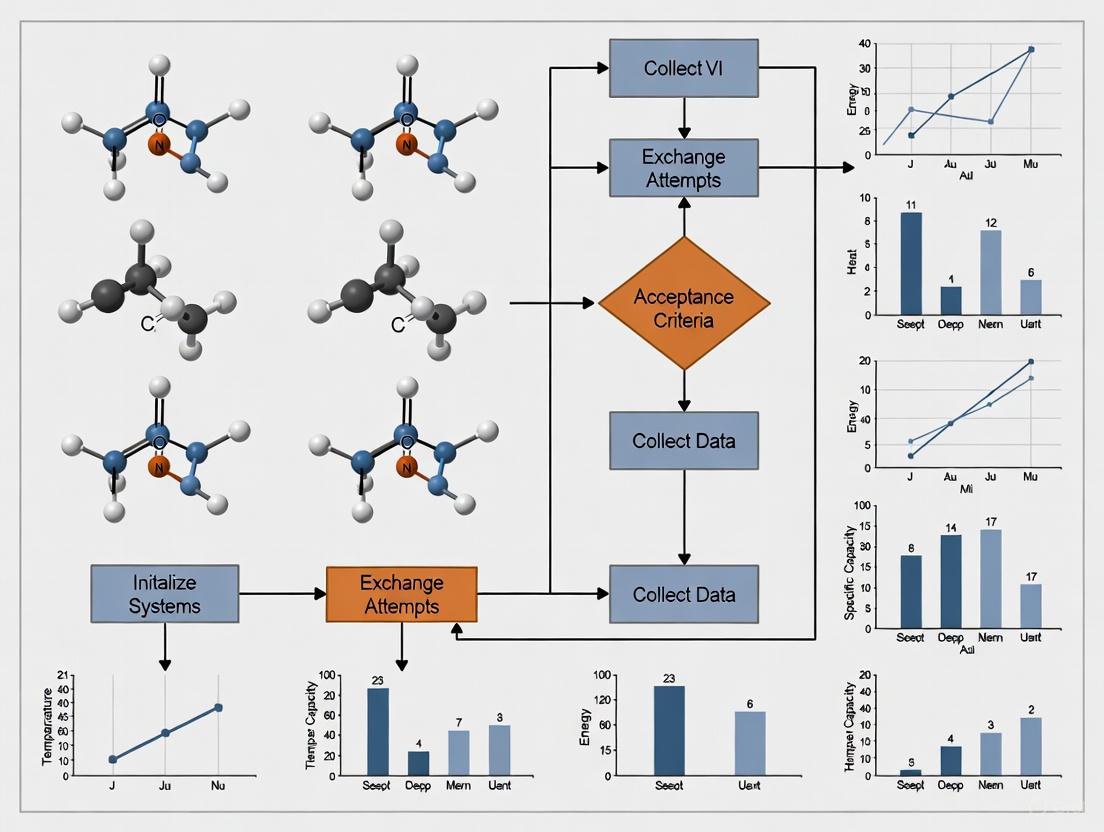
The following workflow diagram summarizes the core PTMC algorithm:
The Scientist's Toolkit: Research Reagent Solutions
Table 2: Key components and their functions in a PTMC study of colloidal clusters. [3]
| Item | Function in the Experiment |
|---|---|
| Morse Potential | Models the short-range attractive component of the effective pair potential, representing depletion forces between colloidal particles. |
| Yukawa Potential | Models the long-range repulsive component of the pair potential, representing screened electrostatic repulsion between charged colloids. |
| Temperature Ladder | The carefully chosen set of temperatures for each replica; enables effective configuration swapping and prevents trapping. |
| Metropolis Criterion | The probabilistic rule used to accept or reject both local configuration moves and global replica swap moves. |
| Heat Capacity (Cv) Calculation | The key thermodynamic property calculated from energy fluctuations; used to identify structural transitions and dissociation events. |
The logical relationship between the system, methodology, and analysis in a PTMC study is shown below:
Frequently Asked Questions
Q1: The exchange rate between my replicas is too low. What parameters should I adjust to improve it? A low exchange rate often indicates poor overlap in the energy distributions of adjacent replicas. To address this:
- Optimize the Temperature Ladder: A geometric series (constant ratio between temperatures) is a common but often suboptimal starting point [4]. The number of required replicas scales with the square root of the system's degrees of freedom [5]. Adjust the temperatures to ensure the exchange probability is between 20-40%. The acceptance probability for a swap between replicas i and j is given by:
p = min(1, exp( (E_i - E_j) * (β_i - β_j) ))whereEis the energy andβ = 1/kT[6] [7]. You may need to derive a custom temperature ladder through preliminary runs [4]. - Increase Sampling: Ensure you run enough Monte Carlo steps between exchange attempts to allow each replica to adequately sample its current temperature. Insufficient sampling can lead to poor energy histogram overlap [8].
- Focus on a Subsystem: For large systems like proteins, consider partial or local replica exchange methods (PREMD/LREMD). These methods only replicate a subset of atoms (e.g., a ligand or protein loop), drastically reducing the number of replicas needed for efficient exchange [5].
Q2: How do I choose the number of replicas and the temperature range for my system? The goal is to have a sufficient number of replicas to ensure a continuous "annealing path" from the highest to the lowest temperature.
- Number of Replicas: This is system-dependent. As a rule of thumb, it should be proportional to the square root of the number of degrees of freedom in your system,
O(f^(1/2)[5]. For instance, a system with 100 degrees of freedom might require around 10 replicas. Theemceelibrary uses an exponential ladder where the highest temperature isT_max = (√2)^(N_temps-1) * T_min[9]. - Temperature Range: The lowest temperature is typically your target (e.g., 300 K for room temperature). The highest temperature should be high enough to flatten the energy landscape, allowing the system to escape deep local minima. A good check is that the highest-temperature replica explores a distribution close to the prior [9]. For a multi-modal Gaussian, the highest temperature should result in an effective Gaussian width that is comparable to the separation between the modes [9].
Q3: My parallel tempering simulation is computationally slow. What are potential bottlenecks and optimization strategies? Performance issues can arise from several areas:
- Synchronization Overhead: In traditional parallel tempering, all replicas must synchronize before an exchange. The entire simulation proceeds at the pace of the slowest replica, which is often the one at the lowest temperature exploring compact, high-energy barrier configurations [4].
- Alternative Algorithm: Consider using Simulated Tempering, where a single simulation performs a random walk in temperature space. This avoids synchronization delays and runs at the average speed across temperatures [4].
- Communication Costs: If running on multiple nodes, the cost of swapping configurations (or temperatures) can be high. For large state spaces, it can be more efficient to swap temperatures between chains rather than the states themselves [6].
- System-Specific Potentials: The cost of evaluating your energy function (e.g., for complex neural network potentials or look-up tables [8]) is a major factor. Profile your code to identify if the bottleneck is in the energy calculation or the parallel tempering mechanics themselves.
Q4: How can I ensure my simulation has sampled all relevant low-energy states, especially when studying phase transitions? Inadequate sampling of configurational space is a common challenge.
- Monitor Replica Trajectories: Track the path of a single replica as it travels through temperatures over time (demultiplexing) [7]. A healthy simulation will show replicas freely diffusing from the highest to the lowest temperatures and back.
- Perform Structural Analysis: Implement post-processing analysis tools. This can include:
- Use Multi-Histogram Analysis: Re-weight energy histograms collected at all temperatures to compute the partition function and derive accurate thermodynamic properties like entropy and heat capacity across the entire temperature range [8].
Q5: Can parallel tempering be applied to protein sequence design, and how is the "energy" defined? Yes, parallel tempering is a viable alternative to simulated annealing for protein design [7].
- Energy Function: In this context, the "energy" is a scoring function that you seek to minimize. This is often a composite score from a structure prediction tool like ESMfold, which can incorporate confidence in structure prediction (pLDDT), globularity, and the minimization of surface hydrophobic residues [7].
- Workflow: Starting from random amino acid sequences, multiple replicas undergo Monte Carlo sampling at different temperatures. Sequences are mutated and accepted/rejected based on the Metropolis criterion. Replica exchanges allow promising sequences to migrate to lower temperatures, facilitating a continuous flow of design candidates [7].
The Scientist's Toolkit: Research Reagent Solutions
The table below lists key computational tools and their functions used in parallel-tempering experiments.
| Research Reagent | Function / Explanation |
|---|---|
| Extended Lennard-Jones Potentials | Models atomic interactions in simple systems like bulk argon or neon clusters [8]. |
| Embedded-Atom Models (EAM) | A more complex potential for metallic systems, providing a better description of bonding [8]. |
| Atomic Neural Network Potentials | A machine-learning potential offering high accuracy and computational efficiency; often has a Fortran interface [8]. |
| ESMfold | A machine learning tool used in protein design to predict 3D structure from sequence and calculate a design score used as the "energy" [7]. |
| Multi-Histogram Method | A post-processing technique that combines energy data from all temperatures to compute the partition function and accurate thermodynamic properties [8]. |
| Common-Neighbor Analysis (CNA) | A structural analysis method used to identify local crystal structures (e.g., FCC, HCP) in atomic systems during phase transitions [8]. |
Experimental Protocol: A Standard Workflow for Parallel Tempering
This protocol outlines a typical workflow for studying thermodynamic properties using the Parallel-Tempering Monte Carlo method.
1. System and Parameter Initialization
- Define the System: Specify the interaction potential (e.g., Lennard-Jones), boundary conditions (e.g., periodic), and the thermodynamic ensemble (e.g., NVT or NPT) [8].
- Set up Replicas: Choose the number of replicas (
M), the temperature range (T_mintoT_max), and initialize the configurations (e.g., random particle positions) [8] [7]. - Define the Temperature Ladder: Create an array of temperatures,
T[1] ... T[M]. An exponential ladder is a common starting point [9].
2. Monte Carlo Sampling Cycle
Each replica performs a standard Monte Carlo simulation at its assigned temperature for a fixed number of steps (N_cycles_between_swap).
- Perturb: Propose a new configuration, often via particle displacement, volume change, or spin flip [8] [10].
- Evaluate: Calculate the change in energy,
ΔE. - Accept/Reject: Apply the Metropolis criterion:
p_accept = min(1, exp(-β ΔE)), whereβ = 1/kT[7].
3. Replica Exchange Cycle After the sampling cycle, attempt to swap configurations between adjacent-temperature replicas.
- Select Pair: Choose a pair of adjacent replicas,
iandj, at temperaturesT_iandT_j[6]. - Calculate Acceptance Probability: Compute the probability for swapping their configurations:
p_swap = min(1, exp( (β_i - β_j) * (E_i - E_j) ))[6] [7]. - Accept/Reject Swap: Draw a random number
R ~ Uniform(0,1). IfR < p_swap, exchange the configurations of replicasiandj[6].
4. Data Collection and Post-Processing
- Collect Data: At intervals, store energies, configurations, radial distribution functions, and other observables for each replica [8].
- Post-Process: After the simulation, use methods like multi-histogram analysis to compute thermodynamic properties across all temperatures [8]. Perform structural analysis on saved configurations to understand sampled states [8].
Parallel Tempering Workflow and Exchange Mechanics
The following diagram illustrates the core mechanics of the parallel tempering algorithm, showing the interaction between replicas at different temperatures.
Core Concepts and Definitions
What is the fundamental mathematical object that defines a pMCMC algorithm?
The operation of a broad class of pMCMC algorithms can be described by a Markovian kernel of the form:
Pα,S,𝒱(q,dq˜)=∑j=0p∫Yαj(q,v)δΠ1∘Sj(q,v)(dq˜)𝒱(q,dv)
In this formulation, q is the current state, 𝒱(q,dv) is the multiproposal mechanism that generates a cloud of proposals, the Sjs are involutive operators acting on an extended phase space, Π1 is the projection onto the first component (e.g., Π1(q,v)=q), and the αjs determine the acceptance probabilities for each proposed state in the cloud. This formulation generalizes the reversible single-proposal Metropolis-Hastings algorithm to a multiproposal setting [11].
How is the "Work Function" conceptualized in the extended phase space formalism?
Within the extended phase space formalism, the "work" of the algorithm is governed by the interplay between the multiproposal mechanism (𝒱) and the involutive operators (Sj). The acceptance probabilities αj are not arbitrary but must be carefully derived to satisfy detailed balance conditions with respect to the target probability distribution μ. The general criteria that ensure ergodicity and reversibility require that these components are chosen such that the resulting Markov chain is unbiased and reversible, fulfilling the condition:
Pα,S,𝒱(q,dq˜)μ(dq)=Pα,S,𝒱(q˜,dq)μ(dq˜)
This ensures the chain preserves the target measure μ [11].
Acceptance Probability Formulations
What is the general form of the acceptance probability for a state swap in Parallel Tempering?
For a replica exchange (or parallel tempering) simulation involving two replicas with configurations c_i and c_j at temperatures T_i and T_j (with corresponding inverse temperatures β_i = 1/(kT_i) and β_j = 1/(kT_j)), the probability for accepting a swap of their configurations is given by:
This is equivalent to:
This formulation ensures that detailed balance is satisfied [2] [10].
What are the necessary and sufficient conditions for the acceptance probabilities in a general multiproposal pMCMC algorithm?
For the general multiproposal kernel Pα,S,𝒱 to be reversible with respect to the target measure μ, the acceptance probabilities α_j must be chosen to satisfy a generalized detailed balance condition. Theorems 2.2, Corollary 2.4, Corollary 2.6, Theorem 2.10, and Theorem 2.11 in the foundational literature provide specific criteria on α_j, S_j, and 𝒱 to guarantee reversibility. For a conditionally independent proposal structure, these conditions simplify, but the general case requires that the acceptance probabilities are set to counteract the bias introduced by the proposal mechanism and the involutions, ensuring that the stationary distribution of the Markov chain is the desired target μ [11].
Table: Key Components of the pMCMC Mathematical Framework
| Component | Mathematical Symbol | Role in the Algorithm |
|---|---|---|
| Target Distribution | μ |
The high-dimensional probability distribution from which we want to obtain samples. |
| Current State | q |
The state of the Markov chain at the current iteration. |
| Multiproposal Mechanism | 𝒱(q, dv) |
A kernel that generates a cloud of p+1 proposals (including the current state) based on q. |
| Involutive Operators | S_j |
A set of maps on the extended space X × Y that are involutions (S_j ∘ S_j = Identity). |
| Projection Operator | Π₁ |
The map that takes an element of the extended space (q, v) and returns the state q. |
| Acceptance Probabilities | α_j(q, v) |
The probability of transitioning to the state Π₁ ∘ S_j(q, v); must be chosen to satisfy detailed balance. |
Experimental Protocols and Implementation
What is a standard protocol for running a Parallel Tempering simulation? A typical protocol, as implemented in the PROFASI software, involves these steps [4]:
- System Definition: Define the system of interest, such as a peptide sequence (e.g.,
*KLVFFAE*). - Replica Initialization: Choose the number of replicas (e.g.,
4), which determines the level of parallelization. - Temperature Ladder: Define the temperature range, typically with a minimum (
tmin) and maximum (tmax) temperature (e.g.,274 Kelvinto374 Kelvin). Temperatures can be distributed in a geometric series or read from a pre-computed file for optimal performance. - Execution: Run the simulation using an MPI command, for example:
mpirun -np 4 profasi_run.mex -S ParTemp -ac 1 "*KLVFFAE*" -tmin "274 Kelvin" -tmax "374 Kelvin" -ncyc 10000. - Swapping: The simulation runs each replica at its assigned temperature, occasionally proposing swaps of configurations between adjacent temperatures based on the Metropolis-Hastings acceptance probability.
How does one implement a multiproposal pMCMC algorithm like mpCN for high-dimensional problems? The multiproposal pCN (mpCN) algorithm is derived from the general pMCMC framework and is designed for high- and infinite-dimensional target measures that are absolutely continuous with respect to a Gaussian base measure [11]. The implementation involves:
- Proposal Cloud: At the current state
q, generate a cloud of multiple proposals{q'_0, q'_1, ..., q'_p}. The proposal mechanism should be tailored to the Gaussian reference measure. - Acceptance Step: Calculate the acceptance probability for each proposal in the cloud using formulas derived from the general pMCMC reversibility theorems. These probabilities will depend on the log-likelihoods (or energies) of the current and proposed states.
- Selection: Select the next state from the cloud of proposals based on the calculated acceptance probabilities.
- Parallelization: Leverage modern high-performance computing architectures (e.g., GPUs) to evaluate the target density and its gradients for all proposals in the cloud simultaneously, as the multiproposal structure is naturally parallelizable.
Troubleshooting Common Issues
What is the recommended target acceptance rate for swap moves in Parallel Tempering, and how can it be achieved?
For parallel tempering, a common target acceptance probability for swaps between chains is 0.234 [12]. Achieving this target often requires careful tuning of the temperature ladder. If the acceptance rate is too low, the temperature increments between adjacent replicas are likely too large, preventing sufficient overlap in their energy distributions. If the acceptance rate is too high, the increments are too small, reducing the efficiency of sampling as chains are too similar. Modern implementations like the one in BEAST2's CoupledMCMC can automatically tune the temperature difference (Delta Temperature) during a run to achieve the desired target acceptance probability [12].
Why might a Parallel Tempering simulation run slower than a simulated tempering simulation? In a Parallel Tempering implementation, all replicas must be kept in sync. The overall progress of the simulation is therefore limited by the speed of the slowest replica. In molecular simulations, lower temperature replicas (which often have more compact structures) can run much slower than high-temperature ones due to more aggressive energy calculations. Consequently, the parallel tempering simulation runs as fast as the slowest, low-temperature replica. In contrast, Simulated Tempering runs all temperatures in a single chain, with its speed being approximately the average speed across all temperatures [4].
How can one diagnose and address poor sampling in multimodal distributions? Poor sampling of multiple modes is a classic problem that pMCMC and Parallel Tempering aim to solve. If certain modes are underrepresented:
- Problem: The temperature ladder may not provide a smooth enough pathway for chains to escape local modes. The highest temperature might not be high enough to allow free exploration of the state space.
- Solution: Increase the number of replicas to create a finer temperature ladder, ensuring better overlap in energy distributions. Extend the maximum temperature to ensure the hottest chain can freely cross all energy barriers. The general pMCMC framework, with its multiproposal mechanisms, can also be more effective than single-proposal methods or running multiple independent chains, as it allows communication between proposals/chains, helping to traverse difficult geometries [11].
Table: Troubleshooting Guide for Common Parallel Tempering Issues
| Problem | Potential Causes | Diagnostic Checks | Solutions |
|---|---|---|---|
| Low Swap Acceptance | Temperature ladder is too sparse; energy distributions have insufficient overlap. | Check calculated acceptance rate is << 0.234. Plot energy histograms for adjacent temperatures. | Increase the number of chains/replicas. Manually optimize the temperature ladder (e.g., using a "tfile"). |
| Slow Simulation Speed | The slowest replica (often the coldest) is a computational bottleneck. | Check for load imbalance; profile time spent per replica. | Use an optimized proposal mechanism for low-T replicas. Consider Simulated Tempering if parallel speedup is insufficient [4]. |
| Poor Mixing in a Specific Replica | The replica is trapped in a local metastable state. | Check time series of energy and order parameters for a single replica; look for high autocorrelation. | Ensure the temperature ladder facilitates "lateral movement." Verify proposal distributions (e.g., step size) are appropriate for that temperature. |
| Failure to Sample All Modes | High-T chains are not hot enough to overcome energy barriers; no pathway for modes to communicate. | Check if samples from all chains are confined to a single mode. | Increase the maximum temperature. Add more chains to the ladder. Consider a multiproposal pMCMC algorithm designed for multimodal targets [11]. |
The Scientist's Toolkit: Research Reagent Solutions
Table: Essential Computational Tools for Parallel Tempering and pMCMC Research
| Tool / Resource | Type | Primary Function | Key Feature / Use Case |
|---|---|---|---|
| MPI (Message Passing Interface) | Library | Enables inter-process communication for running parallel replicas across multiple CPUs or nodes. | Essential for implementing Parallel Tempering, as it allows replicas to run simultaneously and communicate for swap moves [4] [10]. |
| PROFASI | Software Package | A Monte Carlo simulation package for studying protein folding and biophysical properties. | Includes built-in implementations of Parallel Tempering and Simulated Tempering for complex biomolecular systems [4]. |
| BEAST2 with CoupledMCMC | Software Package (BEAST2 Package) | A platform for Bayesian evolutionary analysis via MCMC. | Provides a Parallel Tempering implementation that automatically tunes the temperature difference to a target acceptance rate, simplifying setup [12]. |
| GPU with TensorFlow/CUDA | Hardware/Software | Provides massive parallelization for computationally intensive tasks. | Ideal for scaling pMCMC algorithms that leverage thousands of proposals per step, as the multiproposal structure maps naturally to GPU architectures [11]. |
| Preconditioned Crank-Nicolson (pCN) | Algorithm | A proposal mechanism for MCMC sampling in high- and infinite-dimensional spaces. | The basis for the novel multiproposal pCN (mpCN) algorithm, which is derived from the general pMCMC framework for targets with a Gaussian base measure [11]. |
Frequently Asked Questions (FAQs)
FAQ 1: Why is my Parallel Tempering Monte Carlo (PTMC) simulation failing to achieve convergence in the calculated free energy? Convergence failure in PTMC often stems from poor overlap between the energy distributions of adjacent replicas, preventing efficient random walks in temperature space [2]. To address this, ensure an optimal temperature distribution; the feedback-optimized algorithm can generate an optimal set of simulation temperatures to improve replica round-trip time and enhance sampling [13]. Furthermore, for alchemical free energy calculations, a critical best practice is to inspect for good phase space overlap for all pairs of adjacent lambda states [14].
FAQ 2: How can I identify structural transitions from my PTMC simulation data? Structural transitions can be identified by calculating thermodynamic properties like the heat capacity from the PTMC simulations. Peaks or shoulders on the heat-capacity curve serve as thermodynamic signatures of these transitions [3]. For instance, in the study of charged colloidal clusters, the dissociation transition was characterized by a peak in the heat capacity at T=0.20 (in reduced units) and the appearance of linear structures [3].
FAQ 3: What are the best practices for analyzing alchemical free energy calculations? A robust analysis of alchemical free energy calculations should consist of several key stages [14]:
- Subsampling the data to retain only uncorrelated samples for analysis.
- Calculating free energy differences using multiple estimators (e.g., from Thermodynamic Integration and Free Energy Perturbation) along with their statistical errors.
- Producing textual and graphical outputs of the computed data.
- Inspecting the data for convergence, identifying the equilibrated portion of the simulation, and verifying good phase space overlap between adjacent states.
FAQ 4: My ligand-binding free energy calculation is inaccurate. What sampling issues could be the cause? Inadequate sampling of ligand conformational, translational, and orientational degrees of freedom in the binding site is a common source of error. A proven methodology to enhance convergence is to use restraining potentials. The absolute binding free energy can be decomposed into steps where biasing potentials restraining the ligand's translation, orientation, and conformation (e.g., based on RMSD relative to the bound state) are turned on and off. The effect of these restraints must be rigorously unbiased in the final calculation [15].
Troubleshooting Guides
Issue 1: Poor Replica Exchange in Parallel Tempering
Problem Low acceptance probability for swaps between replicas at different temperatures, leading to simulations that are "stuck" in metastable states and fail to sample the global energy landscape effectively [2].
Diagnosis and Solutions
- Check Temperature Spacing: The acceptance probability for a swap between two replicas at temperatures T_i and T_j is given by
min(1, exp((E_i - E_j)(1/kT_i - 1/kT_j)))[2]. If the energy histograms of adjacent replicas do not sufficiently overlap, the acceptance rate will be low. - Solution: Optimize the set of temperatures. Use a feedback-optimized algorithm that adjusts temperatures to minimize the replica round-trip time in temperature space, ensuring efficient diffusion of replicas from the lowest to the highest temperature and back [13].
- Verify Number of Replicas: Using too few replicas forces wider temperature spacing, reducing overlap. Using too many is computationally inefficient.
- Solution: Select the optimal number of replicas for your system. For a lattice homopolymer study, this was done empirically by measuring the replica's round-trip time for different chain lengths [13].
Issue 2: High Variance in Alchemical Free Energy Estimates
Problem Large statistical errors in the computed free energy differences between the end states of an alchemical transformation.
Diagnosis and Solutions
- Diagnosis: Insufficient Overlap between λ States: The transformation pathway between states is divided into many intermediate λ states. If the conformational spaces of adjacent λ states do not overlap sufficiently, the free energy estimate will be noisy and inaccurate [14].
- Solution: Increase the number of intermediate λ states, particularly in regions where the system's energy changes rapidly. For complex transformations, use a λ-vector that controls different interaction types (e.g., Coulomb and Lennard-Jones) separately [14].
- Diagnosis: Inadequate Sampling of Ligand Pose: In binding free energy calculations, the ligand may not sufficiently sample the bound pose.
- Solution: Apply a restraining potential to the ligand's conformation, based on the root-mean-square deviation (RMSD) relative to the known bound structure, to enforce sampling relevant to the complexed state [15].
The tables below consolidate key parameters and results from referenced studies to serve as a benchmark for your experiments.
Table 1: SALR Potential Parameters for Colloidal Cluster Simulations [3]
| Parameter | Description | Value |
|---|---|---|
| ρ | Controls range of attractive interaction | 30 |
| ϵ_M | Well depth of Morse potential | 2.0 |
| σ | Diameter of colloidal particles | 1.0 |
| κσ | Inverse Debye length (screened electrostatic) | 0.5 |
| ϵ_Y | Strength of Yukawa repulsion | 1.0 |
Table 2: Thermodynamic Signatures in SALR Clusters [3]
| Event | Thermodynamic Signature | Structural Characteristic |
|---|---|---|
| Dissociation | Peak in heat-capacity curve | Appearance of linear and branched structures |
| Structural Transition | Peak or shoulder in heat-capacity curve | Unrolling of Bernal spiral to "beaded-necklace" motifs |
Experimental Protocols
Detailed Methodology: PTMC for Thermodynamic Properties
This protocol outlines the use of Parallel Tempering Monte Carlo to calculate thermodynamic properties like heat capacity and identify structural transitions, as applied to charged colloidal clusters [3].
System Definition:
- Model the cluster energy as a sum of effective pairwise potentials. The total energy is given by:
V_cluster = Σ [V_a(r_i) + V_r(r_i)]whereV_ais an attractive component andV_ris a repulsive component [3]. - For a type II SALR system, use a short-range Morse function for attraction (
V_a) and a long-range Yukawa function for repulsion (V_r) [3]. - Initialize the system with
Ncolloidal particles.
- Model the cluster energy as a sum of effective pairwise potentials. The total energy is given by:
Parameter Setup:
- Replica Configuration: Choose a set of temperatures, optimized for good energy overlap between adjacent replicas [13].
- MC Parameters: Define the number of MC steps, equilibration period, and sampling frequency.
Simulation Execution:
- Run
Ncopies (replicas) of the system in parallel, each at a different temperature [2]. - For each replica, perform standard Monte Carlo sampling (e.g., particle displacement moves) at its assigned temperature.
- Periodically attempt a swap of configurations between two replicas at adjacent temperatures,
T_iandT_j. Accept the swap with probability:p = min(1, exp((E_i - E_j)(1/kT_i - 1/kT_j)))[2].
- Run
Data Analysis:
- Heat Capacity Calculation: Within the canonical ensemble (NVT), compute the heat capacity per particle from the energy fluctuations obtained from the simulations [3].
- Structural Analysis: Monitor structural metrics (e.g., radius of gyration, end-to-end distance) to characterize the clusters present at different temperatures [3] [13]. Correlate changes in these metrics with features in the heat-capacity curve.
Workflow: PTMC for Free Energy
The Scientist's Toolkit
Table 3: Essential Research Reagents and Computational Tools
| Item | Function in the Experiment |
|---|---|
| Parallel Tempering Algorithm | Enhances sampling by allowing replicas at different temperatures to exchange configurations, helping simulations escape metastable states and converge on the global energy landscape [2]. |
| SALR Potential (Morse + Yukawa) | An effective pairwise potential used to model charged colloidal systems; describes the competition between Short-Range Attraction and Long-Range Repulsion that leads to self-assembly of anisotropic structures [3]. |
| Alchemical λ Pathway | Defines a series of intermediate, non-physical states to gradually transform one system into another (e.g., decoupling a ligand from its environment), enabling free energy calculations between end states with little phase space overlap [14]. |
| Restraining Potentials | Biasing potentials applied to a ligand's translation, orientation, or conformation (RMSD) in binding free energy calculations; they improve sampling efficiency and convergence, and their effect is removed analytically in the final result [15]. |
| Free Energy Perturbation (FEP) | A method for estimating free energy differences from simulations by analyzing the energy differences between adjacent states in the alchemical pathway [14]. |
| Thermodynamic Integration (TI) | A method for estimating free energy differences by computing the ensemble average of the derivative of the system's Hamiltonian with respect to the coupling parameter λ [14]. |
Frequently Asked Questions (FAQs)
Q1: My parallel tempering simulation is not achieving good exchange rates between replicas. What could be wrong? Poor exchange rates often stem from an insufficient overlap in the energy distributions of adjacent replicas. This is frequently caused by a poorly chosen temperature set. Ensure your temperatures are spaced to provide a consistent exchange probability (e.g., 20-30%) across all replica pairs. If temperatures are too far apart, the energy distributions will not overlap enough for exchanges to occur. You can diagnose this by plotting the potential energy distributions for each replica; they should significantly overlap with their neighbors [3].
Q2: How can I identify a structural transition from my simulation data? Structural transitions are often signaled by peaks or shoulders in the heat capacity (Cv) curve as a function of temperature [3]. Calculate the heat capacity from the fluctuations in the potential energy. A sharp peak typically indicates dissociation of the cluster at higher temperatures, while more subtle shoulders can signify internal structural rearrangements, such as the unrolling of a Bernal spiral into a beaded-necklace motif [3].
Q3: What is the practical difference between interpolation and extrapolation in this context? Interpolation estimates unknown values within the range of your existing data, such as estimating energy for a temperature between two known simulation points. This is generally reliable. Extrapolation attempts to predict values outside the known range, which is riskier and not recommended for constructing interpolating distributions, as it can lead to mathematically unstable and unreliable results [16] [17].
Q4: My simulation is sampling unrealistic, high-energy structures. How can I guide it better? This can happen if the temperature of a replica is too high, leading to sampling in the dissociative regime. Focus on the lower-temperature replicas, which sample the low-energy structures of interest, such as spherical shapes, Bernal spirals, and beaded-necklace motifs [3]. Also, verify the parameters of your interaction potential to ensure they accurately reflect the physical system you are modeling [3].
Troubleshooting Guides
Problem: Poor Replica Exchange Efficiency A low acceptance rate for swaps between adjacent replicas slows down convergence and hampers the exploration of the energy landscape.
- Diagnosis:
- Calculate and plot the acceptance rate for swaps between each pair of adjacent temperatures.
- Plot the potential energy distributions for all replicas. Look for gaps between the distributions of neighboring replicas.
- Solutions:
- Retune the Temperature Ladder: The most common solution is to adjust the temperatures of your replicas. Use a formula that spaces temperatures geometrically, as the energy variance often increases with temperature. If a geometric progression is insufficient, consider adaptive schemes that dynamically adjust temperatures to achieve uniform exchange rates.
- Increase the Number of Replicas: If the energy landscape is particularly rough, you may need to add more replicas to reduce the energy gap between adjacent temperatures, thereby increasing overlap.
Problem: Failure to Observe Expected Structural Transitions The heat capacity curve is flat and does not show the expected peaks or shoulders that indicate thermodynamic events.
- Diagnosis:
- Check if your temperature range is wide enough. The dissociation transition, for instance, might occur at a higher temperature than you are simulating [3].
- Ensure your simulation has run for enough Monte Carlo steps to adequately sample the relevant configurations.
- Solutions:
- Extend the Temperature Range: Add replicas at higher temperatures to capture dissociation events and at lower temperatures to better resolve low-energy structural transitions.
- Increase Sampling: Run the simulation for longer. Use the integrated autocorrelation time of the energy to estimate the required simulation length.
- Analyze Configurations: Manually inspect snapshots from replicas at different temperatures to classify the structures (e.g., spherical, spiral, linear). This can confirm if a transition is occurring even if the Cv signal is weak [3].
Problem: Inaccurate Interpolation of Data Points When using interpolation to analyze results (e.g., for free energy calculations), the interpolated values are inaccurate or show oscillatory behavior.
- Diagnosis:
- This is a classic sign of applying an inappropriate interpolation method for your data's characteristics.
- Solutions:
- Choose the Correct Method: Select an interpolation technique suited to your data:
- Linear Interpolation: Best for data where you expect a constant rate of change between points. Simple and stable [17].
- Polynomial Interpolation: Can capture more complex, non-linear relationships but can suffer from runaway oscillations (Runge's phenomenon) if the degree is too high [16].
- Spline Interpolation: Often the best compromise, as it fits piecewise low-degree polynomials, creating smooth curves without excessive oscillation [16] [17].
- Cross-Validate: Use techniques like leave-one-out cross-validation (LOOCV) to empirically assess the error of your interpolation method on your specific dataset [16].
- Choose the Correct Method: Select an interpolation technique suited to your data:
Experimental Protocols & Methodologies
Table 1: Key Parameters for a SALR Colloidal Cluster PTMC Simulation
| Parameter | Description | Example Value / Method |
|---|---|---|
| Interaction Potential | A sum of pairwise SALR potentials [3]. | V(r) = V_a(r) + V_r(r) |
| Attractive Component (V_a) | Models depletion attraction; often a Morse potential [3]. | ϵ_M * [e^(ρ(1-r/σ)) * (e^(ρ(1-r/σ)) - 2)] with ϵ_M=2.0, ρ=30, σ=1 [3] |
| Repulsive Component (V_r) | Models screened electrostatic repulsion; often a Yukawa potential [3]. | (ϵ_Y * e^(-κσ(r/σ - 1)))/(r/σ) with ϵ_Y=1.0, κσ=0.5 [3] |
| Number of Replicas | Number of parallel simulations at different temperatures. | 8-64, depending on system size and temperature range. |
| Temperature Set | The temperatures for each replica. | Geometrically spaced, e.g., T = 0.10, 0.15, 0.20, ..., 0.40 [3]. |
| Monte Carlo Steps | Total steps per replica for equilibration and production. | Typically millions to tens of millions. |
| Exchange Attempt Frequency | How often to attempt a swap between replicas. | Every 100-1000 Monte Carlo steps. |
Protocol 1: Setting Up a Basic PTMC Simulation for Thermodynamic Analysis
- System Definition: Define the cluster size (number of particles, N) and the interaction potential with its specific parameters (e.g., M30+Y1.0) [3].
- Replica Initialization: Choose the number of replicas and a set of temperatures. Initialize particle positions for each replica, which could be random, a lattice, or a known low-energy structure.
- Equilibration: Run each replica independently for a sufficient number of Monte Carlo steps to reach equilibrium at its respective temperature. Monitor energies to confirm stability.
- Production Run with Exchanges: Run the parallel tempering simulation, periodically attempting swaps of configurations between adjacent-temperature replicas based on the Metropolis criterion.
- Data Collection: Record the potential energy, configuration snapshots, and acceptance rates for swaps throughout the production run.
Protocol 2: Calculating Heat Capacity and Identifying Transitions
- Energy Time Series: From the production run, extract the time series of potential energy for each replica.
- Heat Capacity Calculation: Calculate the heat capacity per particle (Cv) at each temperature (T) from the energy fluctuations within the canonical ensemble:
Cv = (〈E²〉 - 〈E〉²) / (kT²), whereEis the potential energy,kis Boltzmann's constant, and angle brackets denote ensemble averages [3]. - Plot and Analyze: Plot Cv as a function of T. Identify peaks (signaling dissociation) and shoulders (signaling internal structural transitions) [3].
- Structural Analysis: Correlate features in the Cv curve with structural changes by analyzing saved configuration snapshots from temperatures around the feature.
The Scientist's Toolkit: Research Reagent Solutions
Table 2: Essential Components for SALR Colloidal Simulations
| Item | Function in the Simulation / Experiment |
|---|---|
| Effective Pair Potential (SALR) | The fundamental model describing the isotropic interaction between colloidal particles, combining short-range attraction and long-range repulsion [3]. |
| Morse Potential Parameters (ϵ_M, ρ, σ) | Controls the depth, range, and core diameter of the short-range attractive part of the interaction [3]. |
| Yukawa Potential Parameters (ϵ_Y, κ) | Controls the strength and inverse screening length of the long-range repulsive tail, modeling electrostatic effects in a solvent [3]. |
| Parallel Tempering Algorithm | The enhanced sampling method that facilitates escape from local energy minima by allowing replicas at different temperatures to exchange configurations [3]. |
| Global Optimization Algorithm (e.g., Evolutionary Algorithm) | Used to find the low-energy (e.g., global minimum) structures of the cluster at T=0 K, providing a reference for structures observed in finite-temperature simulations [3]. |
Workflow and System Visualization
PTMC Simulation Workflow for SALR Clusters
SALR Potential Components and Parameters
Implementing Parallel Tempering: Methods and Real-World Applications
Frequently Asked Questions
1. What is the primary purpose of the communication phase in Parallel Tempering? The communication phase, involving replica swap attempts, is crucial for preventing the simulation from becoming trapped in local energy minima. It allows configurations sampled at high temperatures, which can explore the energy landscape more freely, to propagate down to the lower-temperature replicas. This facilitates tunneling through energy barriers and enables a more thorough exploration of the configuration space, which is essential for achieving ergodic sampling in complex, multimodal systems [1] [2].
2. My simulation exhibits low swap acceptance rates between adjacent replicas. What is the most likely cause? Low swap acceptance rates are typically caused by insufficient overlap in the energy distributions of neighboring replicas [2] [18]. This occurs when the temperature spacing in your replica ladder is too wide. To correct this, you should adjust your temperature set to ensure that the difference in average energies between adjacent replicas is approximately equal to the square root of the sum of their energy variances, which generally targets an acceptance rate of 20-30% [18].
3. How does the local exploration phase contribute to the overall sampling? During the local exploration phase, each replica undergoes independent Markov chain Monte Carlo (MCMC) sampling (e.g., using Metropolis-Hastings updates) at its assigned fixed temperature [1] [18]. This phase is responsible for detailed exploration of the local energy basin. The high-temperature replicas broadly survey the landscape, while the low-temperature replicas refine the sampling in deep energy minima, providing high-resolution detail for the target thermodynamic distribution [2] [18].
4. Can Parallel Tempering be used for global optimization, not just sampling? Yes. By using the Boltzmann distribution ( p(x) \propto \exp(-E(x)/kT) ), the modes of the probability density correspond to the minima of the energy function ( E(x) ) [19]. After running Parallel Tempering, the configuration with the lowest energy sampled at the coldest temperature provides an approximation of the global minimum [19]. The algorithm acts as a "super simulated annealing that does not need restart" [2].
Troubleshooting Guides
Problem: Poor Mixing at Low Temperatures
Symptoms: The lowest-temperature replica becomes stuck in a single metastable state for long periods, with a noticeable lack of improvement in the sampled energy and high autocorrelation times.
Solutions:
- Verify Temperature Spacing: Ensure the energy histogram overlap between the coldest replica and the next one is sufficient. The swap acceptance probability is given by ( p = \min\left(1, \exp\left(\Delta\beta \Delta E\right)\right) ), where ( \Delta\beta = 1/(kTi) - 1/(kT{i+1}) ) and ( \Delta E = E{i+1} - Ei ) [1] [2] [18].
- Increase Number of Replicas: Adding more replicas between the current temperature extremes allows for smoother diffusion of configurations from high to low temperatures [18].
- Check Local Moves: Ensure the local MCMC move set (e.g., particle displacement magnitude) is appropriately tuned for each temperature to achieve a good local acceptance rate (~40-60%) [3].
Problem: The Simulation Fails to Converge
Symptoms: Thermodynamic averages, such as mean energy or heat capacity, do not stabilize even after long runtimes.
Solutions:
- Extended Equilibration: Discard a larger portion of the initial sampling data as equilibration. Monitor the time evolution of energies to identify a stable plateau.
- Diagnose Replica Flow: Track the "round-trip time" for a configuration to travel from the lowest temperature to the highest and back. Slow round-trips indicate inefficient mixing and may require more replicas or adjusted temperatures [18].
- Re-initialize Configurations: Start from different, randomized initial conditions to verify that the simulation converges to the same average properties, thus testing for ergodicity.
Problem: Computational Cost is Prohibitively High
Symptoms: The simulation runtime, driven by running many replicas in parallel, is too long for the available resources.
Solutions:
- Optimize Replica Count: The number of replicas needed scales approximately with the square root of the system's degrees of freedom. Use the minimum number that still provides adequate swap acceptance [18].
- Parallelization Efficiency: Ensure the code is efficiently parallelized so that the computational cost of the local exploration phase scales linearly with the number of replicas. The communication overhead for swaps should be minimal.
- Non-Reversible Algorithms: Consider implementing a non-reversible swap scheme (alternating between even-odd and odd-even neighbor pairs), which has been shown to provide up to a 42% improvement in efficiency under optimal conditions [20].
Experimental Protocol & Parameters
The following methodology is adapted from a study investigating structural transitions in charged colloidal clusters, a system with a SALR (short-range attraction, long-range repulsion) potential [3].
Interaction Potential
The total energy of a cluster of ( N ) particles is given by a sum of pairwise potentials: [ V{\text{cluster}} = \sum{i=1}^{N(N-1)/2} \left[ Va(ri) + Vr(ri) \right] ]
- Attractive Component (( Va )): Modeled with a Morse potential for short-range depletion attraction. [ Va(ri) = \epsilonM \left( e^{\rho (1 - ri/\sigma)} \left( e^{\rho (1 - ri/\sigma)} - 2 \right) \right) ]
- Repulsive Component (( Vr )): Modeled with a Yukawa potential for screened electrostatic repulsion. [ Vr(ri) = \epsilonY \frac{e^{-\kappa \sigma (ri / \sigma - 1)}}{ri / \sigma} ]
Default PTMC Parameters (Colloidal Clusters)
The table below summarizes key parameters and their functions from a typical application [3].
| Parameter | Symbol | Value/Type | Function |
|---|---|---|---|
| Potential Type | - | SALR (Type II) | Models competition between short-range attraction and long-range repulsion [3]. |
| Morse Well Depth | ( \epsilon_M ) | 2.0 (reduced) | Controls the strength of the attractive interaction [3]. |
| Morse Range | ( \rho ) | 30 | Governs the range of attraction; higher values mean shorter range [3]. |
| Yukawa Strength | ( \epsilon_Y ) | 1.0 (reduced) | Determines the magnitude of the repulsive charge interaction [3]. |
| Inverse Debye Length | ( \kappa ) | ( 0.5 / \sigma ) | Controls the screening length for the repulsive Yukawa potential [3]. |
| Particle Diameter | ( \sigma ) | 1.0 (reduced) | Defines the length scale of the system [3]. |
| Local Move Sampler | - | Metropolis-Hastings MCMC | Performs local exploration within a single replica [3] [19]. |
| Analysis Metric | - | Heat Capacity vs. Temperature | Identifies thermodynamic signatures of structural transitions and dissociation [3]. |
Workflow Visualization
PTMC High-Level Workflow: This diagram illustrates the two-phase structure of the Parallel Tempering Monte Carlo algorithm, highlighting the cycle between local exploration and global communication.
The Scientist's Toolkit: Research Reagent Solutions
| Item | Function in PTMC Simulation |
|---|---|
| Replica Ladder | A set of simulations at different temperatures (T1 < T2 < ... < TN); the lowest (T1) targets the distribution of interest, while higher temperatures enable barrier crossing [2] [18]. |
| Local MCMC Sampler | The algorithm (e.g., Metropolis-Hastings) that performs stochastic moves (e.g., particle displacements) to explore the local energy landscape of a single replica [1] [19]. |
| Swap Acceptance Criterion | The Metropolis-based rule, ( p = \min(1, \exp((Ei - Ej)(1/kTi - 1/kTj))) ), that determines whether to exchange configurations between two replicas, preserving detailed balance [2] [18]. |
| SALR Potential | An effective pair potential with competing Short-Range Attraction and Long-Range Repulsion, used to model systems like charged colloids and proteins [3]. |
| Heat Capacity Curve | A key thermodynamic property ( C_v ) plotted against temperature; its peaks and shoulders signal structural transitions or dissociation events in the cluster [3]. |
| Convergence Diagnostic | Metrics (e.g., round-trip time, stability of averages) used to determine if the simulation has sufficiently sampled the configuration space [18]. |
Frequently Asked Questions
How many replicas do I need for my system, and how should I space the temperatures? The number of replicas required depends on the system's size and complexity, and the temperature range you need to cover. The temperatures should be spaced to achieve a swap acceptance rate between 20% and 40%, with around 30% often being optimal for efficient sampling [21]. Using too few replicas, or temperatures that are too far apart, will result in low swap rates and poor sampling. Using too many is computationally inefficient.
What is the consequence of a poorly chosen temperature ladder? A poorly chosen temperature ladder can lead to two main problems [21]:
- Low Acceptance Rate (<20%): The replicas do not swap states effectively. The high-temperature replicas cannot help the low-temperature ones escape local energy minima, defeating the purpose of parallel tempering.
- Poor Temperature Space Traversal: Individual replicas may become trapped within a small subset of temperatures, preventing the system from fully exploring the configuration space.
Are there methods to find a good temperature set automatically? Yes, adaptive algorithms exist that dynamically adjust the temperature ladder during sampling. Some aim for uniform acceptance rates between adjacent replicas [22], while more advanced methods use policy gradient reinforcement learning to optimize the temperature spacings to minimize the integrated autocorrelation time of the sampler [22].
What is a simple way to generate an initial temperature ladder? For a first attempt, a geometric temperature distribution (constant ratio between adjacent temperatures) is a common starting point [4] [22]. Online calculators and pre-processing tools are also available, where you input the number of particles, temperature range, and target acceptance probability to generate a proposed temperature set [21].
Troubleshooting Guide
Symptom: Low swap acceptance rate between replicas.
- Diagnosis: The potential energy distributions of adjacent replicas do not have enough overlap. The temperature spacing is likely too wide [23] [21].
- Solution: Increase the number of replicas to reduce the temperature difference between neighbors. Alternatively, if you cannot add more replicas, reduce the maximum temperature (though this may reduce the ability to cross large energy barriers).
Symptom: A replica is trapped in a single temperature or a small subset of temperatures.
- Diagnosis: The replica is not successfully walking through temperature space. This can occur if the swap frequency is too low or if the temperature spacing is non-optimal [21].
- Solution: First, ensure your temperature ladder is well-tuned for a ~30% acceptance rate. If the problem persists, you may need to increase the frequency of swap attempts between replicas.
Symptom: The simulation fails to find the global energy minimum, getting stuck in a local minimum.
- Diagnosis: The highest temperature in your ladder may not be high enough to allow the system to overcome large energy barriers [23].
- Solution: Increase the maximum temperature (
Tmax). As a guideline, the highest-temperature replica should be able to freely traverse the entire energy landscape [23] [21].
Experimental Protocols
Protocol 1: Setting Up a Basic Parallel Tempering Simulation This protocol outlines the steps for a typical parallel tempering simulation using a geometric temperature spacing, as might be implemented in software like LAMMPS or PROFASI [4] [21].
- Define System and Range: Identify your system and define the lower (
Tmin) and upper (Tmax) temperature bounds. - Estimate Replica Count: Use the formula for geometric spacing or an online calculator to estimate the number of replicas
Nneeded for a ~30% acceptance rate. - Generate Temperatures: Calculate the temperature for replica
iusing the formula: ( Ti = T{min} \times \left( \frac{T{max}}{T{min}} \right)^{\frac{i-1}{N-1}} ). - Configure Simulation: Assign each of the
Nparallel processes one temperature from the ladder. - Set Swap Frequency: Choose a frequency for attempting replica swaps (e.g., every 100-1000 Monte Carlo steps or MD steps).
- Run and Monitor: Execute the simulation and monitor the acceptance rates between all adjacent replica pairs.
Protocol 2: Adaptive Temperature Spacing Using Acceptance Rates This methodology, based on contemporary research, dynamically adjusts the temperature ladder to achieve uniform acceptance rates [22].
- Initialization: Start with a preliminary temperature set (e.g., a geometric distribution).
- Equilibration Run: Perform a short parallel tempering simulation.
- Measure Acceptance Rates: Calculate the acceptance rate for swaps between every pair of adjacent temperatures.
- Adjust Temperatures: Apply an adaptive algorithm. A common heuristic is to move temperatures closer if their swap rate is too low and push them apart if the rate is too high [22].
- Iterate: Repeat steps 2-4 until the acceptance rates between all adjacent replicas are approximately equal and within the 20-40% target range.
- Production Run: Use the optimized temperature set for a long, production-level simulation.
The table below summarizes the key parameters for these protocols.
| Parameter | Protocol 1: Basic Setup | Protocol 2: Adaptive Setup |
|---|---|---|
| Number of Replicas | Estimated via calculation [21] | Determined adaptively during initialization |
| Temperature Spacing | Geometric series [4] [22] | Dynamically adjusted to uniform acceptance [22] |
| Target Acceptance Rate | ~30% [21] | Uniform across all pairs (e.g., 20-40%) [22] |
| Swap Frequency | Every 100-1000 steps [21] | Every 100-1000 steps |
| Key Advantage | Simple to implement | Improved sampling efficiency |
Workflow Diagram
The following diagram illustrates the logical workflow for setting up and troubleshooting a parallel tempering simulation.
The Scientist's Toolkit
The table below details key computational reagents and their functions for setting up parallel tempering simulations.
| Research Reagent | Function / Purpose |
|---|---|
| MPI (Message Passing Interface) | Enables parallel computation by managing communication between different replicas running on multiple processors [4] [21]. |
| Temperature Ladder File | A text file containing a sorted list of temperatures (or inverse temperatures) for the replicas, allowing for custom, non-geometric spacing [4]. |
| Langevin Thermostat | A common thermostat used in molecular dynamics simulations to maintain each replica at its specific target temperature [21]. |
| Replica Exchange Log File | The master log file that records the temperature index of each replica at every swap step, essential for analyzing temperature traversal and acceptance rates [21]. |
| Geometric Spacing Calculator | An online or script-based tool that calculates a geometric temperature series given a target temperature range and acceptance probability [21]. |
Troubleshooting Common PTMC Simulation Issues
Q1: My simulation is trapped in a local energy minimum and cannot sample the full configuration space. What should I do?
A: This is a fundamental challenge that Parallel Tempering Monte Carlo (PTMC) is designed to address. The issue arises from a rough energy landscape with high barriers between low-energy states [24].
- Solution: Verify that your temperature ladder is properly configured. The temperatures should be spaced closely enough to ensure a high acceptance probability for replica exchanges (typically 20-30%). If exchanges are too infrequent, add more replicas or adjust the temperature range. Also, ensure that the highest temperature is sufficient to overcome the largest energy barriers in your system [24].
Q2: How can I identify structural transitions or dissociation events from my PTMC data?
A: Thermodynamic properties like heat capacity are excellent indicators. Calculate the heat capacity as a function of temperature from your simulation data [3].
- Solution: Peaks or shoulders in the heat capacity curve often signify thermodynamic events. A strong peak at higher temperatures typically indicates cluster dissociation, while features at lower temperatures can signal internal structural transitions, such as a Bernal spiral unrolling into a beaded-necklace structure [3]. Monitor the populations of different structural motifs (e.g., spherical, spiral, linear) across temperatures to correlate with heat capacity features.
Q3: I want to construct a kinetic model of conformational dynamics, but some states are poorly sampled at the temperature of interest. Can PTMC data help?
A: Yes. A key advantage of PTMC is that data from all temperatures can be integrated. While standard analysis uses data only from the temperature of interest, advanced reweighting techniques allow you to use information from all replicas [25].
- Solution: Implement dynamical reweighting methods. These techniques permit the estimation of transition probabilities and rates at a target temperature by reweighting short trajectory segments from all simulated temperatures, thereby reducing statistical uncertainty and providing estimates for transitions not observed at the temperature of interest [25].
Q4: The acceptance rate for replica exchanges is very low. What parameters can I adjust?
A: A low acceptance rate defeats the purpose of parallel tempering. The primary factor is the overlap in potential energy distributions between adjacent replicas [24].
- Solution: Adjust your temperature ladder. You may need to increase the number of replicas to decrease the temperature spacing between them, especially over temperature ranges where the system's energy changes rapidly. Alternatively, for some systems, tempering in other Hamiltonian parameters (e.g., interaction strengths) might be more efficient.
Thermodynamic Property Analysis Table
The following table summarizes key thermodynamic properties and structural features that can be extracted from PTMC simulations to study transitions, as demonstrated in studies of molecular and colloidal systems.
| Property to Calculate | Technical Method of Calculation | Interpretation of Results | Representative Example from Research |
|---|---|---|---|
| Heat Capacity (Cv) | Fluctuations in potential energy: ( Cv = \frac{ \langle E^2 \rangle - \langle E \rangle^2 }{kB T^2} ) | Peaks indicate major thermodynamic events like dissociation; shoulders suggest subtler structural transitions [3]. | Charged colloidal clusters show a dissociation peak at T=0.20 (reduced units) and lower-T shoulders for spiral-to-necklace transitions [3]. |
| Potential Energy | Direct average of the total energy from sampled configurations at each temperature: ( \langle E \rangle ) | A smooth, monotonic increase with temperature is expected. Sharp jumps can coincide with phase transitions. | Used to compute other derived properties like heat capacity and to monitor the equilibration of the simulation [3]. |
| State Populations | Decompose configuration space into metastable states (e.g., spherical, spiral, necklace) and calculate fractional population at each T [25]. | Reveals temperature-dependent stability of different structures. A crossover in population indicates a structural transition. | In SALR clusters, low-energy Bernal spirals are populated at low T, while linear, dissociated structures dominate at high T [3]. |
| Radial Distribution Function (RDF) | Average density of particles as a function of distance from a reference particle: ( g(r) ) | Reveals changes in short-range order and packing, useful for identifying melting or structural rearrangements. | Not explicitly detailed in results, but a standard analysis for structural changes in clusters and liquids. |
Essential Experimental Protocols
Protocol 1: Setting up a PTMC Simulation for a Biomolecular System
This protocol outlines the steps for simulating a peptide like Met-enkephalin [24].
- System Preparation: Obtain or generate the initial atomic coordinates for the molecule. Place it in a simulated solvent box and add counterions if necessary.
- Parameter Selection:
- Number of Replicas (M): Typically 8-64, depending on the system size and temperature range.
- Temperature Ladder (T1...TM): Choose a maximum temperature high enough to overcome major barriers (e.g., 600K for peptides). Space temperatures to achieve a 20-30% replica exchange acceptance rate [24].
- Energy Function: Use a realistic all-atom force field (e.g., AMBER, CHARMM). The total energy is typically ( E{tot} = E{es} + E{vdW} + E{hb} + E_{tors} ), covering electrostatics, van der Waals, hydrogen bonding, and torsion terms [24].
- Simulation Execution:
- Each replica is simulated in parallel at its assigned temperature using standard Monte Carlo (or Molecular Dynamics) updates.
- After a fixed number of steps (e.g., 100-1000), attempt a swap between configurations of adjacent replicas (e.g., Ti and Ti+1). The swap is accepted with probability ( A = min(1, exp[(\betai - \beta{i+1})(E(C{i+1}) - E(Ci))] ) ), where ( \beta = 1/k_B T ) [24].
- Data Harvesting: Save the trajectory of configurations for each replica for subsequent analysis.
Protocol 2: Analyzing Structural Transitions in Colloidal Clusters
This protocol is adapted from studies of charged colloidal clusters with SALR potentials [3].
- Interaction Potential Definition: Use an effective pair potential that captures the essential physics. A common choice is the sum of a short-range Morse attraction and a long-range Yukawa repulsion:
- Total Energy: ( V{cluster} = \sum{i=1}^{N(N-1)/2} [Va(ri) + Vr(ri)] )
- Morse Attraction: ( Va(ri) = \epsilonM e^{\rho (1 - ri/\sigma)} (e^{\rho (1 - ri/\sigma)} - 2) )
- Yukawa Repulsion: ( Vr(ri) = \epsilonY \frac{e^{-\kappa \sigma (ri / \sigma - 1)}}{ri / \sigma} )
- Parameters (example): ( \rho = 30 ), ( \epsilonM = 2.0 ), ( \sigma = 1.0 ), ( \kappa \sigma = 0.5 ), ( \epsilonY = 1.0 ) (reduced units) [3].
- Global Optimization: Perform a separate global optimization (e.g., using evolutionary algorithms) to identify the lowest-energy structures (e.g., Bernal spirals, beaded-necklaces).
- PTMC Simulation: Run a PTMC simulation as in Protocol 1, but for the cluster system.
- Post-Processing:
- Calculate the heat capacity as a function of temperature.
- Identify all saved configurations and classify them into structural families (e.g., based on their similarity to the global minima found in step 2).
- Plot the population of each structural family versus temperature to identify transition points corresponding to features in the heat capacity curve [3].
The Scientist's Toolkit: Research Reagent Solutions
| Reagent / Computational Tool | Function in PTMC Research |
|---|---|
| Effective SALR Potential | Models the competing short-range attraction and long-range repulsion in colloidal systems, enabling the study of self-assembly into anisotropic structures like Bernal spirals [3]. |
| All-Atom Force Field | Provides a realistic energy function (( E_{tot} )) for biomolecules, accounting for electrostatic, van der Waals, hydrogen-bonding, and torsional interactions, which create the rough energy landscape PTMC aims to navigate [24]. |
| Markov State Model (MSM) | A framework for building a kinetic model of biomolecular dynamics from many short simulation trajectories, which can be enhanced using data reweighted from PTMC simulations [25]. |
| Dynamical Reweighting Algorithm | A computational technique that integrates data from all temperatures in a PT simulation to construct more accurate kinetic models at a specific temperature of interest [25]. |
Workflow and Signaling Diagrams
Frequently Asked Questions (FAQs)
1. What is the primary advantage of combining Parallel Tempering Monte Carlo with electronic structure calculations? This integration enables the efficient exploration of complex energy landscapes and accurate determination of thermodynamic properties for materials and molecular systems. PTMC enhances sampling across energetic barriers by simulating multiple replicas at different temperatures, while electronic structure methods provide the essential energy evaluations with quantum mechanical accuracy [3] [26].
2. My PTMC simulation is not converging. What could be wrong? Poor convergence often stems from an improperly chosen temperature set. Ensure temperatures span a sufficiently wide range to facilitate random walks between low-energy states and fully disordered configurations. For biomolecular systems, a typical range might be 270K to 370K, while materials science applications may require different ranges based on the energy scales involved [27].
3. How do I determine the appropriate number of replicas for my system? The number of replicas depends on system size and complexity. Start with 8-16 replicas, ensuring sufficient overlap between energy distributions at adjacent temperatures. Monitor acceptance ratios for replica exchanges; optimal values typically range between 20-40% [27] [26].
4. Can machine learning accelerate these integrated calculations? Yes, machine learning frameworks like MALA can dramatically accelerate electronic structure calculations by predicting electronic properties using neural networks trained on DFT data. This approach can achieve up to three orders of magnitude speedup, enabling simulations of systems with over 100,000 atoms that would be infeasible with conventional DFT [28] [29].
5. How do I verify the numerical accuracy of my electronic structure computations? Compare results across multiple electronic structure codes with different numerical implementations. For all-electron codes, total energies should agree within 10⁻⁶ using identical exchange-correlation functionals. Monitor convergence thresholds for density (typically 10⁻⁶) and total energy (10⁻⁸ Hartree/Rydberg) [30].
Troubleshooting Guides
Poor Replica Exchange Acceptance Rates
Symptoms:
- Replicas become trapped at specific temperatures
- Low acceptance rate for configuration exchanges between adjacent temperatures
Solutions:
- Adjust Temperature Spacing: Use a geometric progression for temperature distribution. For example: 270K, 280K, 295K, 310K, 325K, 340K, 355K, 370K [27]
- Increase Replica Count: Add more replicas to reduce gaps between temperature levels
- Modify Exchange Attempt Frequency: Adjust the
T_update_intervalparameter if using PROFASI or equivalent in other packages [27]
Inaccurate Energy Evaluations
Symptoms:
- Erratic thermodynamic averages
- Unphysical structural transitions in heat-capacity curves [3]
Solutions:
- Verify Electronic Structure Parameters:
- For all-electron codes: Check basis set completeness and convergence parameters [30]
- Ensure consistent treatment of exchange-correlation functionals across all replicas
- Validate Energy Differences: Compare energy differences between structures with multiple codes when possible [30]
Memory and Performance Issues in Large Systems
Symptoms:
- Excessive computational time for energy evaluations
- Memory limitations with increasing system size
Solutions:
- Implement Machine Learning Acceleration:
- Optimize Parallelization:
- Use multiplexing when available to enhance replica exchange efficiency [27]
- Distribute replicas across CPU cores with appropriate load balancing
Experimental Protocols
Standard Protocol for PTMC with Electronic Structure Calculations
System Preparation:
- Define the atomic system and initial configuration
- Select appropriate interaction potential or electronic structure method
- For colloidal systems, use established SALR potentials with Morse and Yukawa terms [3]
Temperature Setup:
- Determine temperature range covering relevant physical processes
- Create temperature set with geometric progression
- Verify sufficient overlap between adjacent distributions
Simulation Execution:
- Initialize all replicas with different configurations
- Set convergence criteria for electronic structure calculations
- Run parallel simulation with periodic replica exchange attempts
Data Collection:
- Monitor replica trajectories and exchange statistics
- Calculate thermodynamic observables (heat capacity, structural metrics)
- Verify convergence through multiple independent runs
Specialized Protocol for Large-Scale Systems with Machine Learning
Training Phase:
- Generate reference data with DFT calculations on small systems (256 atoms)
- Train neural networks to map atomic environments to local density of states [28]
- Validate model predictions against held-out DFT data
Production Phase:
- Apply trained ML model to predict electronic structure in PTMC
- Calculate energies and forces from predicted electronic properties
- Perform PTMC sampling with ML-accelerated energy evaluations
Computational Setups for Different System Types
Table 1: Representative Parameter Sets for Various Applications
| System Type | Temperature Range | Replicas | Electronic Structure Method | Key Parameters |
|---|---|---|---|---|
| Colloidal Clusters [3] | T=0.20 (reduced units) | 8-16 | SALR potential (Morse + Yukawa) | ρ=30, εM=2.0, εY=1.0 |
| Protein Folding [27] | 270K-370K | 8 | Force field or QM/MM | loglevel=10, numcycles=5M |
| Large Materials [28] [29] | System-dependent | 8-32 | MALA ML-DFT | Bispectrum descriptors, neural network inference |
| Metallic Systems [30] | Varies with lattice parameter | 8-16 | All-electron DFT (Wien2k/FPLO) | Rkmax=4-12, PBE functional |
Research Reagent Solutions
Table 2: Essential Computational Tools and Their Functions
| Tool/Software | Primary Function | Application Context |
|---|---|---|
| PROFASI [27] | Parallel Tempering implementation | Biomolecular simulations with replica exchange |
| MALA [28] [29] | Machine learning for electronic structure | Large-scale materials simulations beyond DFT limits |
| Wien2k [30] | All-electron DFT calculations | High-accuracy electronic structure reference data |
| FPLO [30] | Full-potential local-orbital method | Efficient all-electron calculations with precision |
| LAMMPS [29] | Molecular dynamics simulator | Descriptor calculation and force evaluation |
| Quantum ESPRESSO [29] | DFT electronic structure | Training data generation and method validation |
Workflow Visualization
PTMC-Electronic Structure Workflow
Performance Optimization Parameters
Table 3: Critical Numerical Parameters for Accuracy and Efficiency
| Parameter | Recommended Value | Purpose | Source |
|---|---|---|---|
| Density Convergence | 10⁻⁶ | Electronic structure self-consistency | [30] |
| Energy Convergence | 10⁻⁸ Hartree/Rydberg | Total energy accuracy | [30] |
| Replica Exchange Frequency | Every 10-100 MC sweeps | Balance between sampling and overhead | [27] |
| Temperature Update Interval | 10 MC sweeps | Optimize communication patterns | [27] |
| Basis Set Size (Wien2k) | Rkmax=4-12 | Control numerical accuracy/precision trade-off | [30] |
| k-point Sampling | Tetrahedron method with Blöchl corrections | Accurate Brillouin zone integration | [30] |
Troubleshooting Guides & FAQs
Troubleshooting Common Computational Challenges
FAQ: My Parallel-Tempering Monte Carlo (PTMC) simulation fails to achieve adequate sampling of ligand binding modes. What could be wrong?
- Problem: Inadequate sampling of ligand binding modes in PTMC simulations.
- Explanation: PTMC enhances sampling by running multiple replicas of the system at different temperatures. Inefficient exchange between replicas or insufficiently broad temperature range can trap simulations in local energy minima, preventing exploration of key binding poses [31].
- Solution:
- Verify Temperature Distribution: Ensure your temperature ladder allows for a sufficient acceptance probability for replica exchanges (typically 20-30%). You may need to adjust the number of replicas or the temperature range [31].
- Check Simulation Length: Confirm that the total simulation time is long enough to observe multiple binding and unbinding events, or transitions between known binding modes.
- Validate Force Field: Review the energy function. Using a hierarchy of energy functions—a simplified model for robust landscape exploration and a more accurate force field for final energy quantification—can improve results [31].
FAQ: How can I improve the accuracy of binding free energy estimates from my simulations?
- Problem: Inaccurate binding free energy estimates.
- Explanation: Binding free energy is the central thermodynamic quantity for ligand affinity. Traditional end-point methods like MM/PBSA and MM/GBSA contain approximations, such as the neglect of conformational entropy and the treatment of solvation, which can limit accuracy [32] [33]. Force field inaccuracies, particularly in atomic charges, also contribute to error [33].
- Solution:
- Incorporate Advanced Electrostatics: Substitute force field atomic charges with those derived from QM/MM calculations on ligand-bound conformations. This better accounts for polarization effects in the binding site [33].
- Use Multi-Conformer Protocols: Employ methods that consider multiple low-energy conformers (e.g., mining minima) for free energy processing instead of relying on a single pose [33].
- Apply a Universal Scaling Factor: A scaling factor (e.g., 0.2) can be applied to calculated free energies to correct for systematic overestimation and improve agreement with experimental data [33].
FAQ: My structure-based affinity prediction performs poorly when no experimental protein-ligand structure is available. What are my options?
- Problem: Poor performance of docking-based affinity prediction without high-resolution co-crystallized structures.
- Explanation: Many accurate affinity prediction models depend on known 3D binding structures. In their absence, performance drops significantly [34].
- Solution: Implement a computational pipeline that predicts the structure before estimating affinity.
- Fold the Protein: Use deep learning-based protein structure prediction tools (e.g., ColabFold) to generate an apo protein structure from its amino acid sequence [34].
- Dock the Ligand: Employ a deep learning-based docking model (e.g., DiffDock) to predict the binding pose of the ligand into the predicted protein structure [34].
- Predict Affinity: Use a 3D graph neural network on the predicted protein-ligand binding structure to estimate the binding affinity. This Folding-Docking-Affinity (FDA) framework provides a viable alternative when experimental structures are lacking [34].
Table 1: Performance Comparison of Binding Free Energy Estimation Protocols on a Benchmark of 9 Targets and 203 Ligands [33]. MAE: Mean Absolute Error; Rp: Pearson Correlation Coefficient.
| Method / Protocol | MAE (kcal mol⁻¹) | Rp | Key Characteristic |
|---|---|---|---|
| QCharge-MC-FEPr | 0.60 | 0.81 | QM/MM charges on multiple conformers with Free Energy Processing |
| QCharge-VM2 | 0.68 | 0.74 | QM/MM charges on the most probable conformer, then new search |
| MM-VM2 (Classical) | ~1.20 | ~0.60 | Classical force field atomic charges (estimated from context) |
| FEP (Reference) | 0.80 - 1.20 | 0.50 - 0.90 | Alchemical free energy perturbation, computationally intensive [33] |
| MM/PBSA (Reference) | Varies Strongly | Varies Strongly | Performance is highly system-dependent [32] |
Table 2: Virtual Screening Performance (Pearson Correlation - Rp) of the FDA Framework on Kinase Datasets [34].
| Test Scenario | DAVIS (FDA) | DAVIS (Docking-Free ML) | KIBA (FDA) | KIBA (Docking-Free ML) |
|---|---|---|---|---|
| Both-new | 0.29 | ~0.27 (DGraphDTA) | 0.51 | ~0.49 (DGraphDTA) |
| New-drug | 0.34 | ~0.34 (MGraphDTA) | 0.44 | ~0.43 (MGraphDTA) |
| New-protein | 0.32 | ~0.28 (DGraphDTA) | 0.46 | 0.48 (MGraphDTA) |
| Sequence-identity | 0.38 | ~0.33 (DGraphDTA) | 0.45 | 0.47 (MGraphDTA) |
Experimental Protocols & Workflows
Protocol 1: Binding Free Energy Estimation using QM/MM and Multi-Conformer Sampling [33]
Aim: To accurately estimate the absolute binding free energy for a protein-ligand system. Principle: This protocol combines the thoroughness of the mining minima (M2) method, which identifies multiple low-energy conformers, with the accuracy of quantum mechanics/molecular mechanics (QM/MM)-derived electrostatic potential (ESP) charges. Procedure:
- Classical Conformer Search: Perform an initial "classical" mining minima (MM-VM2) calculation using a molecular mechanics force field to identify an ensemble of low-energy protein-ligand conformers and their associated probabilities.
- Charge Refinement: Select the most probable conformers (e.g., those covering >80% of the probability). For each, perform a QM/MM calculation where the ligand is treated with quantum mechanics and the protein with molecular mechanics. Fit new ESP atomic charges for the ligand based on this electronic structure calculation.
- Free Energy Processing (FEPr): Replace the original force field charges in the selected conformers with the new QM/MM-derived ESP charges. Recalculate the binding free energy using the Free Energy Processing step of the M2 method on this charge-corrected ensemble of conformers.
- Scaling and Validation: Apply a universal scaling factor (γ=0.2) to the calculated free energies to offset systematic bias. Validate the predicted binding free energies against experimental measurements.
Protocol 2: Folding-Docking-Affinity (FDA) Framework for Affinity Prediction [34]
Aim: To predict protein-ligand binding affinity when a co-crystallized 3D structure is unavailable. Principle: Leverage recent advances in AI-based protein structure prediction and molecular docking to generate a putative 3D binding structure, which is then used for affinity prediction. Procedure:
- Folding: Input the protein's amino acid sequence into a protein folding tool (e.g., ColabFold) to generate a predicted tertiary structure (apo form).
- Docking: Input the generated protein structure and the ligand's molecular representation (e.g., SMILES) into a deep learning-based docking tool (e.g., DiffDock) to predict the most likely binding pose, forming a complete protein-ligand complex.
- Affinity Prediction: Pass the predicted 3D binding structure to a 3D graph neural network (e.g., GIGN) to compute a quantitative estimate of the binding affinity.
Methodology and Workflow Visualization
The Scientist's Toolkit: Research Reagent Solutions
Table 3: Essential Computational Tools and Resources for Protein-Ligand Binding Studies.
| Tool / Resource | Type / Category | Primary Function |
|---|---|---|
| Parallel Tempering/Replica Exchange | Sampling Algorithm | Enhances conformational sampling by running parallel simulations at different temperatures, facilitating escape from local energy minima [31]. |
| QM/MM (e.g., ESP Charges) | Energy Calculation | Provides more accurate electronic structure-derived atomic charges for ligands in a protein environment, improving electrostatic interaction energy estimates [33]. |
| Mining Minima (M2) | Free Energy Method | A statistical mechanics framework for binding affinity prediction that identifies and weights multiple low-energy conformers, bridging the speed of docking and rigor of FEP [33]. |
| AlphaFold/ColabFold | Protein Structure Prediction | AI-based tools that predict 3D protein structures from amino acid sequences, invaluable when experimental structures are unavailable [34]. |
| DiffDock | Molecular Docking | A deep learning model that predicts the binding pose of a ligand to a protein structure with high speed and accuracy [34]. |
| PDBBind Database | Curated Dataset | A collection of high-resolution crystallographic protein-ligand complexes with experimentally measured binding affinity data, used for training and validation [34] [35]. |
| ChemBL Database | Bioactivity Database | A large-scale database of bioactive molecules with drug-like properties and their annotated targets, used for pretraining models on protein-ligand interactions [35]. |
Optimizing Parallel Tempering Performance: Solving Common Challenges
Replica Exchange Molecular Dynamics (REMD) and its Monte Carlo variant, Parallel Tempering, are powerful enhanced sampling techniques used to accelerate the exploration of complex energy landscapes, such as those encountered in biomolecular systems and materials science. These methods operate by running multiple parallel simulations (replicas) at different temperatures or with different Hamiltonians, periodically attempting to swap their configurations. The core idea is that higher-temperature replicas can overcome large energy barriers more easily, and this improved sampling can be propagated down to the lower temperatures of interest via successful exchanges. However, the effectiveness of these methods is critically dependent on achieving good "mixing"—the efficient and random walk of replicas through temperature space. When mixing is poor, sampling is hindered, and results can be unreliable. This guide provides a structured approach to diagnosing the common bottlenecks that lead to poor mixing in replica exchange simulations.
FAQ: Diagnosing Poor Mixing
1. What are the primary symptoms of poor replica exchange mixing?
The most common symptoms include a low acceptance ratio for replica exchange attempts, replicas that become "trapped" at certain temperatures for long periods, and poor convergence of thermodynamic properties. A key quantitative metric is the replica round-trip time, which measures the time for a replica to travel from the lowest temperature to the highest and back. Long round-trip times indicate slow mixing and inefficient sampling.
2. How do I know if my temperature spacing is appropriate?
The acceptance probability for exchanges between neighboring replicas is governed by the overlap of their potential energy distributions. According to the GROMACS manual, for a system with all bonds constrained ( Number of degrees of freedom, ( N{df} \approx 2 N{atoms} )), the relative temperature spacing ( \epsilon ) should be chosen as approximately ( 1/\sqrt{N_{atoms}} ) to maintain a reasonable acceptance rate [36]. Many MD software packages offer online calculators to help determine an optimal temperature set based on your system size and temperature range.
3. Why does my system size affect mixing, and what can I do about it?
As system size increases, the number of degrees of freedom grows, causing the potential energy distributions at different temperatures to become narrower and overlap less. This leads to a rapid decrease in exchange acceptance rates [36] [37]. To maintain efficiency, the number of replicas must often be increased in proportion to the square root of the number of degrees of freedom, which can become computationally expensive [37]. For very large systems, consider advanced methods like Replica Exchange Statistical Temperature Monte Carlo (RESTMC) or Hamiltonian replica exchange, which can be more efficient [36] [37].
4. How frequently should I attempt replica exchanges?
Exchanges should be attempted as frequently as possible without incurring significant communication overhead in parallel computing environments. The interval should be short compared to the timescale of the slow conformational transitions you wish to enhance [38] [39]. For molecular dynamics, a typical exchange attempt interval is every 100 to 1000 simulation steps.
Troubleshooting Guide: Common Bottlenecks and Solutions
Symptom: Low Acceptance Ratio
A low acceptance ratio for exchange attempts is a direct indicator of poor overlap between replicas.
- Cause 1: Inadequate Temperature Spacing. The temperatures of neighboring replicas are too far apart.
- Solution: Add more replicas to reduce the temperature spacing. Use a tool like the GROMACS REMD calculator to generate a better temperature distribution [36].
- Cause 2: Incorrect Order of Replicas. In standard REMD, exchanges are typically only attempted between neighboring temperatures. If the replicas are not correctly ordered by temperature, the exchange mechanism will fail.
- Solution: Ensure your simulation input files correctly assign an ordered set of temperatures to the replicas.
- Cause 3: System Size Effects. As explained in the FAQ, larger systems naturally require more replicas for a given temperature range.
- Solution: Increase the number of replicas or switch to a method like Hamiltonian replica exchange, which can be less sensitive to system size [37].
Symptom: Replicas Trapped at Extreme Temperatures
This occurs when a replica gets stuck at the highest or lowest temperature for an extended period, failing to perform a random walk through temperature space.
- Cause: Large Free Energy Barriers at the Temperature Extremes. The highest temperature may not be high enough to sufficiently destabilize deep energy minima, or the lowest temperature may be too cold for the system to escape a stable state.
- Solution: Widen the overall temperature range or adjust the number of replicas. Ensure the highest temperature is sufficiently high to cause frequent unfolding or crossing of major barriers [10].
Symptom: Poor Convergence of Thermodynamic Averages
Even with a reasonable acceptance ratio, the estimates of properties like free energy or heat capacity may not converge.
- Cause: Infrequent Exchange Attempts Relative to Internal Dynamics. If exchanges are attempted too rarely, the beneficial sampling from high temperatures does not propagate efficiently to low temperatures.
- Cause: Underlying Slow Dynamics at the Temperature of Interest. Replica exchange accelerates sampling but does not eliminate the intrinsic timescales of the system.
- Solution: Run longer simulations. Use the efficiency gain formula, ( \eta ), to estimate the required simulation length compared to standard MD [39].
Diagnostic Tables
Table 1: Symptoms, Causes, and Diagnostic Checks for Poor Mixing
| Symptom | Primary Causes | Key Diagnostic Checks |
|---|---|---|
| Low Acceptance Ratio | - Temperature spacing too wide- System size too large for chosen parameters | - Calculate acceptance probability between all neighbor pairs- Check if ( \epsilon \approx 1/\sqrt{N_{atoms}} ) [36] |
| Trapped Replicas | - Insufficient temperature range- Free energy barriers too high | - Monitor replica trajectory vs. simulation time- Plot replica index as a function of simulation time |
| Poor Convergence | - Exchange attempts too infrequent- Total simulation time too short | - Check exchange attempt frequency vs. correlation times- Calculate statistical error/replica round-trip time [39] |
Table 2: Typical Parameter Ranges for Efficient Replica Exchange
| Parameter | Typical Target Range | Comments and References |
|---|---|---|
| Acceptance Ratio | 20% - 40% | A higher rate is not always better, as it may indicate wasted replicas with overly tight temperature spacing [36]. |
| Number of Replicas, (N) | ( N \propto \sqrt{f} ) | Scales with the square root of the number of degrees of freedom, (f) [37]. |
| Relative Temp Spacing, ( \epsilon ) | ( \approx 1/\sqrt{N_{atoms}} ) | For a protein/water system with constrained bonds [36]. |
| Exchange Frequency | As high as computationally feasible | Should be fast compared to the system's slowest relaxation time [38] [39]. |
Experimental Protocols for Diagnosis
Protocol 1: Quantifying Replica Mixing Efficiency
- Simulation: Run a parallel tempering simulation for a fixed number of exchange attempts.
- Data Collection: Log the temperature (or Hamiltonian) index for each replica at every exchange attempt.
- Analysis:
- Acceptance Ratio: Calculate the average acceptance probability for exchanges between all neighboring temperature pairs.
- Replica Trajectory: For each replica, plot its temperature index as a function of simulation time or exchange attempt number. This visualizes trapping.
- Round-Trip Time: Measure the average time for a replica to start at the lowest temperature, reach the highest, and return to the lowest.
Protocol 2: Estimating Efficiency Gain for Two-State Systems
For systems whose long-time dynamics are dominated by transitions between two states (e.g., folded/unfolded), the relative efficiency of REMD versus standard MD can be quantified [39].
- Run Simulations: Perform a REMD simulation and a standard MD simulation at your temperature of interest, ( T_m ), using equivalent computational resources.
- Measure Lifetimes: For each temperature ( Ti ) in the REMD simulation, estimate the average lifetimes in the two states, ( \taui^+ ) and ( \taui^- ). Do the same for the MD simulation at ( Tm ) (( \taum^+ ), ( \taum^- )).
- Calculate Efficiency: The relative efficiency is given by: [ \etam = \frac{1}{N} \sum{i=1}^N \frac{\taum^+ + \taum^-}{\taui^+ + \taui^-} ] An ( \etam > 1 ) indicates REMD is more efficient than standard MD for sampling at ( Tm ) [39].
Workflow Visualization
Diagnostic Workflow for Replica Exchange Bottlenecks
The Scientist's Toolkit: Research Reagent Solutions
Table 3: Essential Components for a Parallel Tempering Study
| Item | Function in the Experiment | Technical Specifications / Notes |
|---|---|---|
| Temperature Set | Defines the ensemble for each replica. | A set of temperatures, often geometrically spaced, covering a range from the target low temperature to a sufficiently high temperature. |
| Hamiltonian Pathway (for H-REMD) | Defines the altered potential energy function for each replica in Hamiltonian exchange. | A series of λ-states that morph the system from one state to another (e.g., from solute in vacuum to solvated) [36]. |
| Exchange Protocol | Governs the rules for swapping replica states. | Includes the exchange attempt frequency and the pairing scheme (e.g., even-odd pairs) [36]. |
| Efficiency Metrics | Quantifies the performance and sampling quality of the simulation. | Includes acceptance ratio, replica round-trip time, and statistical error of target observables [39]. |
| Analysis Tools | Used to post-process simulation data and compute thermodynamic properties. | Tools for weighted histogram analysis (WHAM), calculation of heat capacity, and visualization of replica walks. |
Frequently Asked Questions (FAQs)
1. What is the primary advantage of using a non-linear annealing schedule over a linear one in Parallel Tempering Monte Carlo (PTMC)?
A linear schedule, where temperature changes at a constant rate, often fails to account for the varying "roughness" of the energy landscape. Non-linear schedules are optimized to spend more computational time where the system's thermodynamic properties change most rapidly, such as near phase transitions. This leads to more efficient sampling, reduced systematic error in estimating properties like heat capacity, and a higher probability of finding the global energy minimum [3] [41].
2. My PTMC simulation is not achieving good replica exchange rates. How can path optimization in parameter space help?
Low acceptance rates indicate that adjacent replicas in your temperature (or parameter) stack are too dissimilar. An optimized path ensures that the "distance" between successive replicas is small enough for meaningful exchange. The formalism of a "friction tensor"—derived from the time correlation of the forces conjugate to your control parameters—allows you to construct a geodesic path in parameter space. This path maintains a near-constant thermodynamic distance between replicas, maximizing the overall exchange rate and improving sampling efficiency [41].
3. How do I handle multiple control parameters, like inverse temperature and an external field, in an advanced annealing schedule?
Traditional annealing only varies temperature (β). Advanced path optimization generalizes this to a trajectory in a multidimensional space (e.g., β, J, h). The optimal schedule is found by defining a metric tensor based on correlations between the conjugate forces (e.g., energy, magnetization). The annealing path is then a geodesic with respect to this metric, ensuring a smooth and efficient transition through the combined parameter space [41].
4. What are the signs of ergodicity breaking in my simulation, and how can the schedule be adjusted to mitigate it?
Ergodicity breaking often manifests as the population of replicas getting trapped in a subset of low-energy states, leading to poor convergence of thermodynamic averages. This is common near first-order phase transitions or in glassy systems. If your system has known metastable states, you can design the annealing path to intentionally pass through regions of parameter space that lower the barriers between these states, facilitating transitions [41].
5. Can these advanced scheduling techniques be used for optimization (finding ground states) as well as for thermodynamic sampling?
Yes. Schedules that minimize statistical error for thermodynamic sampling also perform well for optimization when the target is a sufficiently low temperature. The key for both is efficiently navigating the energy landscape to avoid metastable traps. An optimized schedule reaches the low-temperature, ground-state-dominant region more reliably than a simple linear anneal [41].
Troubleshooting Guides
Problem: Poor Replica Mixing and Low Exchange Rates
A low acceptance rate for replica swaps indicates inefficient exploration of the energy landscape.
- Step 1: Diagnose the Issue. Calculate the average acceptance probability between all pairs of adjacent replicas in your stack. Identify where the rate drops significantly.
- Step 2: Apply Path Optimization. Use the following methodology to construct an improved schedule:
- Formalism: The optimal path minimizes the total dissipation, which is related to the Fisher information. The schedule is governed by the "friction tensor" or metric tensor, g, with components given by:
g_μν(λ) = ∫₀^∞ dt 〈δF_μ(t) δF_ν(0)〉_λwhereF_μ = - ∂E(σ, λ) / ∂λ_μis the generalized force conjugate to control parameterλ_μ, and the average is taken at a fixed point λ in parameter space [41]. - Implementation: For a system where you only control inverse temperature (β), the conjugate force is the energy, and the metric component is proportional to the heat capacity. An optimal schedule will spend more time at temperatures where the heat capacity is high.
- Protocol:
- Perform a short preliminary run with a linear or educated-guess schedule.
- From this data, estimate the metric tensor g across your parameter range.
- Use an optimization algorithm to find a path (schedule) that maintains a constant "thermodynamic speed"
√(dλ/dt • g • dλ/dt).
- Formalism: The optimal path minimizes the total dissipation, which is related to the Fisher information. The schedule is governed by the "friction tensor" or metric tensor, g, with components given by:
- Step 3: Validate. Run your PTMC simulation with the new schedule and re-calculate the swap acceptance rates. They should be more uniform and higher overall.
Problem: Failure to Converge in Heat Capacity Calculations
The calculated heat capacity curve may show high variance or miss peaks if the schedule does not properly sample critical regions.
- Step 1: Identify Critical Regions. Look for large fluctuations in energy or other order parameters in your initial results. These regions often coincide with structural transitions or dissociation events [3].
- Step 2: Implement a Multi-Stage Schedule. Instead of a single annealing protocol, design a schedule with denser replica spacing in the identified critical temperature regions. For example, if a heat capacity peak is observed near
T=0.20for a colloidal cluster, the replica density around this temperature should be increased [3]. - Step 3: Adaptive Protocol. For long-running simulations, consider an adaptive approach. Periodically calculate the heat capacity or energy variance from recent data and automatically adjust the replica distribution for the next run to focus on the most uncertain regions.
Problem: Managing Computational Cost with Multiple Parameters
Adding more control parameters (e.g., chemical potential, field strength) exponentially increases the number of possible replicas, making the simulation computationally prohibitive.
- Solution: Hybrid and Quantum-Augmented Methods. Offload the most computationally expensive parts of the sampling process.
- Quantum-AFQMC: In Quantum Auxiliary-Field Quantum Monte Carlo (qAFQMC), a quantum computer is used to prepare and sample complex trial wavefunctions that are intractable for classical computers. This reduces the bias and variance in energy estimates for a given computational budget on the classical hardware [42].
- Hybrid Solver Workflow: As explored in quantum annealing, a hybrid workflow can be established where a classical computer handles the overall PTMC coordination, while a specialized quantum processor (or other hardware accelerator) is used to evaluate the energy and generalized forces for difficult configurations [43].
Experimental Protocols & Data
Protocol 1: Calculating an Optimal 1D Temperature Schedule
This protocol outlines how to move from a linear temperature schedule to an optimized one for a PTMC simulation.
- Preliminary Run: Execute your PTMC simulation using a linear temperature schedule between your chosen
T_maxandT_min. Use enough replicas to ensure initial, albeit low, swap rates. - Calculate Heat Capacity: For each replica at its fixed temperature
T_i, calculate the average energy<E>and the heat capacityC_v = (〈E²〉 - 〈E〉²) / T². - Define the Metric: In one dimension (temperature), the metric is
g = C_v / T². This determines the thermodynamic distance between temperatures. - Optimize the Schedule: Solve for the temperature distribution
{T_i}that ensures the integral of√g dTis equal between all adjacent replicas. This creates a schedule with constant thermodynamic speed. - Execute Production Run: Run your main PTMC simulation using this new, optimized set of temperatures.
Quantitative Comparison of Annealing Techniques
The table below summarizes key metrics for different annealing approaches, highlighting the potential benefits of advanced path optimization.
| Algorithm / Technique | Key Control Parameter | Optimal Schedule Principle | Reported Advantage / Performance |
|---|---|---|---|
| Classical Simulated Annealing (SA) | Temperature (T) | Logarithmic decrease (theoretically optimal) | Foundational method, but often impractically slow [41]. |
| Parallel Tempering (PTMC) | Temperature (T) | Linear or geometric spacing | Enables escape from local minima; efficiency highly schedule-dependent [3]. |
| Path Optimized PTMC | Multidimensional (λ) | Geodesic path based on friction tensor | Superior performance: Reduces statistical error and finds lower energies in spin glass simulations compared to linear schedules [41]. |
| Population Annealing (PA) | Temperature (T) | Constant thermodynamic speed | More efficient resampling; outperforms SA in finding ground states of spin glasses [41]. |
| Quantum Annealing (D-Wave Hybrid) | Quantum & Classical | Proprietary hybrid scheduler | Advantageous for specific problems: Shows potential for integer quadratic objectives but has not yet surpassed classical leaders (e.g., CPLEX, Gurobi) for general MILP problems [43]. |
The Scientist's Toolkit: Essential Research Reagents
This table lists key computational "reagents" and their functions in advanced PTMC studies.
| Research Reagent / Tool | Function in Advanced PTMC |
|---|---|
| Friction Tensor (g_μν) | A metric defining thermodynamic distance; the core object for calculating optimal annealing paths in parameter space [41]. |
| SALR Potential | A model interaction potential with Short-Range Attraction and Long-Range Repulsion; used to study self-assembly of colloidal clusters and proteins [3]. |
| Quantum Trial State | A wavefunction prepared on a quantum computer; used in hybrid QMC methods to reduce bias and variance in ground state energy calculations [42]. |
| QUBO Formulation | A Quadratic Unconstrained Binary Optimization problem; the native input format for quantum annealers, allowing them to be applied to discrete optimization problems [43]. |
| Slater Determinant | An anti-symmetrized product wavefunction; represents "walker" states in Auxiliary-Field QMC (AFQMC) and can be efficiently manipulated on classical and quantum computers [42]. |
Workflow and Relationship Visualizations
PTMC with Optimized Schedule Workflow
Multidimensional Parameter Annealing Path
Frequently Asked Questions (FAQs)
Q1: What is the primary advantage of combining neural samplers with Parallel Tempering? The primary advantage is significantly improved sampling efficiency for complex, high-dimensional, and multimodal distributions, commonly encountered in thermodynamic property research. Neural samplers, such as normalizing flows and diffusion models, create more effective "bridges" between the reference and target distributions. This enhances the overlap between adjacent distributions in the annealing path, which in turn facilitates better state swapping and accelerates communication across the entire system, leading to more efficient exploration of the energy landscape [44] [45].
Q2: My Neural Accelerated PT experiment is experiencing mode collapse. What are the common causes and solutions? Mode collapse, where the sampler fails to explore all relevant modes of the posterior, is a known challenge for neural samplers.
- Cause: The neural sampler itself may be mode-collapsing, providing poor-quality proposals that do not represent the full target distribution [45].
- Solutions:
- Leverage PT Framework: The structure of Parallel Tempering itself helps mitigate this. Ensure your annealing path has a sufficient number of levels to create a smooth transition between modes [45].
- Check Training Data: If using a pre-trained flow or diffusion model, verify that the training data adequately represents all known modes of your system.
- Intermittent Training: As suggested in one approach, use a local MCMC (like HMC) to explore modes initially, then train the normalizing flow on these draws to generate better Metropolis proposals, creating a feedback loop for improved mode coverage [46] [47].
Q3: How can I manage the high computational cost of neural networks during sampling? While neural samplers are computationally expensive, the APT framework is designed to use them strategically to minimize overall cost.
- Parallelization: The APT algorithm runs multiple chains in parallel. The neural samplers are also utilized in parallel for proposing swaps, circumventing their serial computational burden [44] [45].
- Multilevel Strategies: For diffusion models, consider a Multilevel Monte Carlo (MLMC) strategy. This approach uses a hierarchy of models with varying costs and accuracies, cleverly coupling them to reduce the overall computational cost of Monte Carlo integration without sacrificing final accuracy [48].
- Architecture Choice: In high-dimensional settings (e.g., d > 10,000), the cost of normalizing flows can be prohibitive. Assess whether the payoff is worthwhile for your problem's dimensionality [47].
Q4: My swap acceptance rates between tempering levels are low. How can I improve them? Low swap acceptance rates indicate insufficient overlap between adjacent distributions.
- Optimize the Annealing Path: Revisit the schedule of your inverse temperatures (( \beta )). A non-linear path, as opposed to a simple linear interpolation, might provide a better progression from the reference to the target distribution [45].
- Leverage Neural Transports: This is the core innovation of APT. The neural samplers are explicitly used to propose more intelligent swaps between states at different temperatures, directly addressing the overlap problem and leading to higher acceptance rates than classical PT [45].
Q5: My normalizing flow is not training stably or fails to learn the posterior. What should I do? Training generative models on complex posteriors is non-trivial.
- Alternative Training Loss: Instead of using the reverse KL divergence, which can be unstable, explore training with the forward KL divergence. This requires samples from the posterior, which can be generated by using the normalizing flow to assist a local MCMC algorithm, creating a self-improving training cycle [46].
- Intermittent Training: Do not train the flow from scratch on a highly complex target. Use the method of assisting a local MCMC to gather initial samples and iteratively train the flow [46] [47].
- Incorporate Importance Sampling: Even a flow with artifacts can be effective when its samples are refined with importance weighting to produce final, unbiased estimates [47].
Troubleshooting Guides
Issue: Poor Global Mixing and Inefficient Mode Hopping
Symptoms:
- The MCMC chain gets trapped in a single mode for a large number of iterations.
- Low effective sample size (ESS) for key thermodynamic observables (e.g., free energy, mean energy).
- The swap acceptance rate between the highest temperature (reference) and lowest temperature (target) chains is near zero.
Diagnostic Steps:
- Visualize Chains: Plot the traces of the chains across all tempering levels for a key parameter. Trapped chains will show no movement between distinct values.
- Quantify Overlap: Calculate the acceptance rate for swaps between every pair of adjacent levels. A sharp drop between two specific levels indicates a poor bridge.
- Check Neural Sampler Quality: Generate independent samples from your neural sampler (flow/diffusion) and check if they visually or quantitatively (e.g., via statistical tests) represent the expected modes.
Resolution Procedures:
- Procedure 1: Increase Annealing Levels
- Add more intermediate distributions to the annealing path to create a smoother transition.
- Use a non-linear temperature schedule that places more levels in regions where the swap rate is lowest [45].
Procedure 2: Refine the Neural Sampler
- If the neural sampler is not capturing all modes, retrain it with a more diverse set of initial states or a different training strategy (see FAQ Q5) [46].
- Ensure the architecture of the neural sampler (e.g., number of layers in a flow, network size in a diffusion model) is sufficiently expressive for your target distribution.
Procedure 3: Validate the Reference Distribution
- Confirm that your reference distribution (e.g., Gaussian) is easy to sample from and that the neural sampler can reliably map from this base distribution.
Issue: Excessive Computational Time or Memory Usage
Symptoms:
- Experiment runtime is prohibitively long.
- Memory errors occur, especially when using large neural network models.
Diagnostic Steps:
- Profile Code: Identify the bottleneck. Is it the local MCMC steps, the neural network evaluations, or the communication between chains?
- Monitor Hardware: Check if you are hitting GPU or CPU memory limits.
Resolution Procedures:
- Procedure 1: Optimize Neural Network Usage
- Use the APT framework's parallel design: run the neural samplers concurrently with the MCMC chains to avoid idle processors [44] [45].
- For diffusion models, integrate the Multilevel Monte Carlo (MLMC) method to reduce the number of expensive neural function evaluations (NFEs) required for accurate Monte Carlo estimates [48].
Procedure 2: Adjust Model Complexity
- For problems with very high dimensionality (d >> 10,000), consider if a simpler neural sampler architecture can be used, or if the method is appropriate for the scale of the problem [47].
- Explore techniques like pruning or quantization for the neural networks to reduce their computational footprint [48].
Procedure 3: Tune Local MCMC
- Ensure that the local MCMC steps (e.g., HMC, MALA) on each tempering level are well-tuned. Inefficient local exploration will force the neural sampler to work harder.
Experimental Protocols & Data
Detailed Methodology: Neural Accelerated Parallel Tempering (APT)
The following protocol outlines the integration of neural samplers into a Parallel Tempering framework for sampling from a complex thermodynamic posterior ( \pi(x) \propto \exp(-U(x)) ).
1. Pre-experiment Setup:
- Define Annealing Path: Establish a sequence of ( N+1 ) distributions ( \pi^0, \pi^1, \dots, \pi^N ) interpolating between a tractable reference ( \pi^0 = \eta ) (e.g., a Gaussian) and the target ( \pi^N = \pi ). A common choice is ( U^n(x) = (1-\betan) \log \eta(x) + \betan U(x) ), with ( 0 = \beta0 < \beta1 < ... < \beta_N = 1 ) [45].
- Select Neural Sampler: Choose and (if necessary) pre-train a neural sampler (e.g., a Normalizing Flow or Diffusion Model) capable of sampling from and evaluating densities for the distributions along the path.
2. Algorithm Initialization:
- Initialize states ( {X0^0, X0^1, ..., X_0^N} ) for each level, often by sampling from the reference ( \pi^0 ).
3. Iteration Loop (for t = 1 to total iterations):
- a. Local Exploration: For each chain ( n ) (in parallel), perform one or several steps of a local MCMC kernel (e.g., Hamiltonian Monte Carlo) that leaves ( \pi^n ) invariant. This yields a new state ( X_t^n ) [45].
- b. Neural Communication (Swapping):
- For a pair of adjacent levels ( (n-1, n) ), use the neural sampler to propose a swap. Instead of a simple state exchange, the neural sampler generates a transport map, creating more informed proposals [44] [45].
- Accept or reject the swap with a Metropolis-Hastings probability that preserves the joint distribution of all chains. The acceptance probability for a neural-guided swap is calculated as: ( \alpha = \min\left(1, \frac{\pi^{n-1}(xt^n) \pi^n(xt^{n-1})}{\pi^{n-1}(xt^{n-1}) \pi^n(xt^n}) \cdot J\right) ) where ( J ) is the Jacobian determinant accounting for the transformation by the neural transport (for flows) [45].
4. Post-processing:
- Use samples from the target chain ( {X_t^N} ) to compute thermodynamic observables via Monte Carlo integration.
- Estimate the change in free energy ( \Delta F = \log Z0 - \log ZN ) using the collected swap statistics and work values from the annealing path [45].
The table below summarizes key quantitative findings from research on neural-accelerated sampling methods.
| Method | Comparison Baseline | Performance Improvement | Key Metric | Application Context |
|---|---|---|---|---|
| Accelerated PT (neural transports) [45] | Classical Parallel Tempering | Improved sample quality, reduced computational cost | Swap Acceptance Rate, Effective Sample Size | Multimodal sampling problems |
| Normalizing Flow-assisted MCMC [46] | Standalone MCMC (e.g., HMC, MALA) | Accelerated mixing rate, better exploration | Mixing Rate, Mode Coverage | Bayesian posteriors with difficult geometry |
| Multilevel Monte Carlo with Diffusion [48] | Standard Diffusion Model Sampling | 4x to 8x reduction in computational cost | Computational Cost (NFEs) | Bayesian inverse problems, computational imaging |
| Normalizing Flow-assisted Nested Sampling [49] | Standard Nested Sampling | Reduced convergence time, better parameter space exploration | Convergence Time, Evidence Estimation | Particle physics model parameter space (Type-II Seesaw) |
Research Reagent Solutions
This table details essential computational "reagents" used in Neural Accelerated PT experiments.
| Item Name | Function / Role in the Experiment |
|---|---|
| Normalizing Flows (e.g., RealNVP) | A neural network that defines an invertible transformation between a simple base distribution and a complex target. It is used to generate high-quality proposals for state swaps in PT and can reshape the posterior for more efficient sampling [46] [49]. |
| Diffusion Models (e.g., DDPM) | A generative model that learns to reverse a gradual noising process. It can be used to sample from the target posterior and is particularly effective for high-dimensional data like images. Can be integrated into MLMC strategies [48]. |
| Controlled Diffusions | Extends diffusion models by incorporating control mechanisms, potentially leading to more efficient sampling paths and proposal generation within the APT framework [44]. |
| Hamiltonian Monte Carlo (HMC) | A local MCMC kernel used for the "exploration" phase within each tempering level. It efficiently explores local geometry by simulating Hamiltonian dynamics [47] [45]. |
| Annealing Path / Schedule (( \beta )) | The sequence of inverse temperatures defining the intermediate distributions. A well-chosen path is critical for ensuring sufficient overlap between levels to enable effective swapping [45]. |
Workflow and System Diagrams
Diagram 1: Neural Accelerated PT High-Level Workflow
Diagram 2: Neural Transport Swap Mechanism
Frequently Asked Questions
FAQ 1: Why is the choice of temperature set critical in Parallel Tempering Monte Carlo simulations?
The temperature set is fundamental because it directly controls the efficiency of replica exchanges. Successful Parallel Tempering (PT) relies on configurations performing a random walk across the entire temperature space [50]. If the temperatures are too widely spaced, the energy distributions of adjacent replicas will not overlap sufficiently. This leads to a low acceptance probability for replica exchanges, causing configurations to become trapped at specific temperatures. This trapping prevents the low-temperature systems from accessing the beneficial high-temperature sampling, and the simulation can become "stuck" in metastable states, defeating the core purpose of the PT algorithm [2].
FAQ 2: What is a common symptom of a poorly spaced temperature set during a simulation?
A clear symptom is a low and uneven replica exchange rate between adjacent temperatures. You may observe that exchanges between some temperature pairs are frequently accepted, while between others, they are rarely accepted. This indicates that the energy histogram overlap is inconsistent across the temperature range. Furthermore, you can monitor the "lateral" movement of a single replica; if it fails to diffuse to the highest and lowest temperatures and back over the course of the simulation, the temperature set is likely suboptimal [50].
FAQ 3: What are the main categories of methods for optimizing the temperature set?
Approaches for finding an optimal temperature set can be divided into two principal categories [51]:
- Constant Swap-Ratio Methods: These methods aim to distribute the replicas so that the acceptance probability for swaps between all neighboring replicas is constant and independent of the temperature values.
- Feedback-Optimized Methods: These techniques, such as the feedback-optimized method, aim for a temperature distribution that has a higher density of replicas at simulation "bottlenecks." This results in temperature-dependent replica-exchange probabilities and seeks to maximize the flow of replicas from the highest to the lowest temperature.
FAQ 4: Does problem type influence which temperature-setting method is most effective?
Yes, the nature of the problem's energy landscape can influence the best method. For systems with a continuous (second-order) phase transition, such as spin glasses, methods that produce a uniform swap rate often perform adequately. However, for problems with a first-order (discontinuous) phase transition, like the fully-connected Wishart model, the feedback-optimized method has been shown to provide a significant performance advantage, sometimes cutting the time-to-solution by a factor of two or more [51].
Troubleshooting Guides
Problem: Low and Inconsistent Swap Acceptance Rates Between Replicas
This is a primary indicator of poor temperature spacing, where the energy distributions of adjacent replicas do not have sufficient overlap.
Solution: Implement the "Spring" Algorithm to Equalize Acceptance Probabilities
This method efficiently tunes the temperature set to achieve a constant swap probability between all neighboring replicas [50].
- Step 1: Run Preliminary Simulations. Conduct short initial Monte Carlo simulations (without replica exchanges) at a preliminary set of temperatures (e.g., an evenly spaced set). The number of replicas and the highest and lowest temperatures are fixed at this stage.
- Step 2: Collect Energy Data. From these simulations, gather energy data to construct histograms ( H{\betai}(E) ) for each inverse temperature ( \betai = 1/Ti ).
- Step 3: Calculate Overlap. Compute the overlap ( O{i, i+1} ) between the energy histograms of every pair of adjacent temperatures ( (\betai, \beta{i+1}) ). This overlap is proportional to the expected swap probability ( P{ij} ) between them.
- Step 4: Optimize Temperature Spacing. Adjust the temperatures as if they were masses connected by springs. The "spring" between two adjacent temperatures ( \betai ) and ( \beta{i+1} ) is assigned an equilibrium length proportional to ( 1/O_{i, i+1} ). The system of springs is then relaxed to find the new, optimized temperature set that equalizes the overlap (and hence the swap probability) across all pairs.
- Step 5: Validate. Run a short PT simulation with the new temperature set to confirm that the swap acceptance rates are now high and uniform.
The workflow for this method is outlined in the following diagram:
Problem: Slow Diffusion of Replicas from Highest to Lowest Temperature
Even with decent local swap rates, replicas may not travel efficiently across the entire temperature range.
Solution: Consider a Feedback-Optimized Method for Challenging Landscapes
This approach explicitly maximizes the probability that configurations drift from the coldest to the hottest temperatures and back [50] [51].
- Step 1: Define a Flux Function. During a preliminary PT run, track the movement of replicas. For each temperature ( Tk ), define a flux function ( f(Tk) ) based on ( n{up}(Tk) ) and ( n{down}(Tk) ), which are the normalized fractions of configurations traveling from the coldest to the hottest temperature and vice versa.
- Step 2: Maximize the Current. The goal is to adjust the temperature distribution density ( \eta(T) ) to maximize a "current" ( j ), defined as ( j = D(T) \eta(T) (df/dT) ), where ( D(T) ) is a diffusivity.
- Step 3: Adjust Temperatures. The temperature set is iteratively refined to achieve this maximized current, which effectively places more replicas in temperature regions where the random walk of replicas is slowest (the bottlenecks).
The logical relationship between the problem symptoms and the choice of solution can be visualized as follows:
The table below summarizes key methods based on the search results.
| Method | Core Principle | Key Metric | Reported Performance |
|---|---|---|---|
| Constant Swap-Ratio [50] | Equalize the acceptance probability for swaps between all neighboring replicas. | Uniform swap rate. | Effective for spin-glass problems with continuous phase transitions [51]. |
| Feedback-Optimized [50] [51] | Maximize the current/diffusion of replicas across the entire temperature range by adding more replicas at bottlenecks. | Constant drift velocity of replicas. | Time-to-solution speedup of at least 2x on Wishart problems with first-order phase transitions [51]. |
| Geometric Progression | Simple geometric spacing between temperatures. | Simple to implement. | Can be inefficient, especially if the system's specific heat diverges [50]. |
The Scientist's Toolkit: Research Reagent Solutions
The table below details key components for a typical PTMC study as referenced in the search results.
| Item | Function in PTMC Simulation |
|---|---|
| Effective Pair Potential (SALR) | Models the interaction between particles (e.g., colloids). It combines short-range attraction and long-range repulsion to produce complex self-assembled structures [3]. |
| Morse Potential | A common choice for the attractive component (( V_a )) of the pair potential. Its parameters control the well depth and interaction range [3]. |
| Yukawa Potential | Often used for the repulsive component (( V_r )) of the pair potential. It models screened electrostatic repulsions, such as those in charged colloidal systems [3]. |
| Spin Glass Hamiltonian | A model Hamiltonian (e.g., Edwards-Anderson) used as a testbed for evaluating the performance of PTMC and temperature-setting algorithms on systems with rough energy landscapes [50] [51]. |
| Energy Histogram | Data structure collected during preliminary simulations. The overlap between histograms at adjacent temperatures is the fundamental data used for tuning temperature sets in several algorithms [50] [2]. |
Frequently Asked Questions (FAQs)
FAQ 1: What is the primary computational challenge that Parallel Tempering Monte Carlo (PTMC) addresses? PTMC is designed to overcome the problem of sampling bottlenecks in complex energy landscapes. In standard Monte Carlo simulations, systems can become trapped in local energy minima (metastable states) at low temperatures, leading to poor sampling and long correlation times. PTMC addresses this by running multiple replicas of the system at different temperatures, allowing configurations to escape local minima via higher-temperature replicas and thus achieve more efficient sampling and better convergence of thermodynamic properties [23] [2].
FAQ 2: How do I determine the number of replicas and the temperature set for my PTMC simulation? The number of replicas and the temperature range are critical for efficiency. The highest temperature must be sufficient to avoid trapping in any local minima, while the lowest temperature is typically the temperature of interest for study [23]. The temperatures should be chosen to ensure a sufficient overlap in the potential energy distributions of adjacent replicas. A common rule of thumb is that the acceptance probability for replica exchanges should be around 20-30% [2]. Temperatures are often spaced in a geometric series [27], and the number of replicas required increases with the system size and the roughness of its energy landscape.
FAQ 3: What is the difference between Parallel Tempering and Simulated Tempering? Parallel Tempering runs multiple replicas simultaneously in parallel, each at a different, fixed temperature. Periodically, configuration swaps between adjacent temperatures are attempted [10] [2]. In contrast, Simulated Tempering runs a single simulation where the temperature itself becomes a dynamic variable that changes during the simulation according to Monte Carlo rules [10]. Parallel Tempering is generally easier to parallelize on modern computing clusters, while Simulated Tempering runs in series.
FAQ 4: Can PTMC be used for purposes other than calculating thermodynamic properties? Yes. While frequently used to compute thermodynamic averages and identify phase transitions (e.g., via heat capacity peaks [3]), PTMC is also a powerful tool for global optimization. The high-temperature replicas can find new low-energy states and feed them to the low-temperature replicas, effectively acting as a sophisticated global optimizer that does not require restarting, akin to a super simulated annealing algorithm [19] [2].
Troubleshooting Guides
Problem: Low Replica Exchange Acceptance Rate
A low acceptance rate indicates poor "mixing" between replicas, meaning configurations are not diffusing effectively across the temperature ladder.
Diagnosis and Solutions:
Check Temperature Spacing:
- Symptoms: Acceptance rate is consistently below 10% for most adjacent replica pairs.
- Solution: Adjust your temperature set to increase the overlap in energy distributions. This typically means adding more replicas to reduce the temperature gap between them [23] [2]. The goal is an acceptance rate of 20-30% for swaps between neighboring replicas.
Verify Energy Overlap:
- Symptoms: Uncertainty in thermodynamic observables (e.g., heat capacity) remains high even after long simulation times.
- Solution: During a preliminary run, histogram the potential energy for each replica. Visually confirm that the histograms for adjacent replicas have significant overlap. If not, add more replicas in the regions of poor overlap [2].
Review Exchange Attempt Frequency:
- Symptoms: The system seems to mix, but the convergence of low-temperature observables is still slow.
- Solution: The interval between exchange attempts should be chosen carefully. Attempting exchanges too frequently (before the replicas have decorrelated) or too infrequently (missing opportunities to swap) can both hinder efficiency. A common practice is to attempt exchanges every 10-100 Monte Carlo sweeps [27].
Problem: Simulation is "Stuck" or Failing to Sample Key States
The low-temperature replicas are not visiting all relevant metastable states, such as different morphologies in colloidal clusters [3].
Diagnosis and Solutions:
Increase Maximum Temperature:
- Symptoms: High-temperature replicas also appear trapped and are not exploring a diverse set of configurations.
- Solution: The highest temperature (Tn) might be too low. It must be high enough to overcome the largest energy barriers in the system, allowing the replica to perform a nearly random walk across the entire configuration space [23]. Increase Tn until the highest-temperature replica shows rapid state changes.
Extend Simulation Time:
- Symptoms: The lateral movement of a configuration from the highest temperature to the lowest is a diffusion process. If the simulation is too short, this process may not complete.
- Solution: The total number of Monte Carlo cycles must be long enough to allow for many round trips of a configuration from the highest to the lowest temperature and back. Monitor the replica index of a configuration over time to ensure these round trips are occurring [2].
Check for Implementation Errors:
- Symptoms: Acceptance rates are zero or anomalously high (e.g., >80%).
- Solution: Verify the correctness of the acceptance probability calculation for swaps. For a swap between replicas
iandj(withiat temperature Ti and configuration Xi, andjat Tj and Xj), the correct Metropolis acceptance probability is [23] [2]:p_acc = min(1, exp( (E_i - E_j) * (1/k_B T_i - 1/k_B T_j) ))where E_i is the energy of configuration Xi at its temperature.
Problem: Inefficient Resource Allocation and Poor Scaling
The computation is running, but the cost in CPU hours is not yielding proportional improvements in sampling quality.
Diagnosis and Solutions:
Optimize the Number of Replicas:
- Symptoms: Computational cost is high, but the gain in sampling efficiency is minimal.
- Solution: The number of required replicas scales with the square root of the system's number of degrees of freedom. Using too many replicas is wasteful, while too few prevents efficient swapping. Find the minimum number of replicas that still provides adequate acceptance rates [2]. The following table summarizes the key parameters to balance:
Profile Computational Cost:
- Symptoms: The simulation is slow, and the bottleneck is not obvious.
- Solution: Use profiling tools to identify if the cost is in the energy evaluation or the communication overhead for replica exchanges. For large systems, the energy calculation will dominate, so optimizing this part of the code is crucial. For systems with fast energy evaluations, the communication overhead of PTMC may become significant.
Leverage Multiplexing (if supported):
- Symptoms: You have access to many more CPU cores than you have replicas.
- Solution: Some PTMC implementations (e.g., PROFASI) support "multiplexing," where multiple replicas run at the same temperature. During an exchange attempt, a replica at T0 can attempt to swap with any of the replicas at a neighboring temperature T1, which can further enhance sampling by increasing the connectivity within the temperature ladder [27].
Experimental Protocols
Standard Protocol for a PTMC Simulation
This protocol outlines a typical workflow for a PTMC study of thermodynamic properties, as applied in systems like colloidal clusters [3] or surface models [52].
- System Initialization: Define the interaction potential and initial configuration for all replicas. Initial configurations can be random, stretched, or based on an imported structure (e.g., a PDB file) [27].
- Temperature Ladder Setup: Determine the number of replicas (
N) and the set of temperatures {T1, T2, ..., TN}, with T1 being the temperature of interest and TN the highest temperature. A geometric progression is a common starting point [27]. - Equilibration: Run each replica independently at its assigned temperature for a sufficient number of Monte Carlo cycles (
num_therm_cycles) to reach equilibrium before initiating replica exchanges [27]. - Production Run with Exchanges:
- Perform a sequence of Monte Carlo sweeps on each replica.
- Periodically (e.g., every
T_update_intervalsweeps), attempt a replica exchange. For each pair of adjacent replicas (i, i+1), calculate the swap acceptance probabilityp_accand decide to accept or reject the swap based on the Metropolis criterion [23] [2]. - Continue for the total number of cycles (
num_cycles).
- Data Collection: Throughout the production run, record observables (energy, heat capacity, structural order parameters, etc.) for each temperature. Configuration snapshots may also be saved periodically (
conf_write_freq) [27]. - Analysis: Analyze the data to compute thermodynamic averages and identify transitions (e.g., by locating peaks in the heat capacity curve [3]). Monitor the replica index history to ensure good "round-trip" behavior between temperature extremes.
Workflow Diagram
PTMC Simulation Workflow
The Scientist's Toolkit: Research Reagent Solutions
The table below details key computational "reagents" and their functions in a typical PTMC study, as derived from research on colloidal clusters and biological molecules.
| Item/Component | Function & Explanation | Example/Value |
|---|---|---|
| Interaction Potential | Defines the energy of a configuration. The SALR (Short-Range Attraction, Long-Range Repulsion) potential is common for charged colloids [3]. | V(r) = Morse_attraction(r) + Yukawa_repulsion(r) [3] |
| Temperature Ladder | The set of temperatures for the replicas. Enables tunneling through energy barriers. | Geometric series, e.g., T = [280, 295, 310, 325, 340, 355, 370] K [27] |
| Replica Exchange Acceptance | Metropolis criterion for swapping configurations between replicas. The core of PTMC that enables sampling enhancement [23] [2]. | p_acc = min(1, exp(Δ))Δ = (E_i - E_j)*(1/kB T_i - 1/kB T_j) |
| Order Parameter | A measurable quantity that characterizes a state or phase transition. Essential for data analysis. | Radius of Gyration (Rg), Protein RMSD, Nativeness (Q) [27], Heat Capacity [3] |
| MPI (Message Passing Interface) | A library specification for parallel computing. Used to run replicas on different processors and manage communication for replica exchanges [10] [27]. | mpirun -np 8 ./ParTempRun.mex [27] |
Replica Exchange Mechanism Diagram
Replica Exchange Process
Validating and Benchmarking Parallel Tempering Against Alternative Methods
Frequently Asked Questions
Q1: My parallel tempering simulation appears to be "stuck" in local optima. How can I improve sampling of multiple modes?
Parallel tempering is particularly susceptible to getting trapped when the temperature ladder is improperly configured. This occurs because chains cannot effectively exchange configurations if their energy distributions don't sufficiently overlap [2].
Solution: Implement a well-designed temperature ladder and monitor swap acceptance rates:
- Ensure adjacent chains have energy histogram overlaps of 20-30% for effective configuration swaps [2].
- Aim for uniform swap acceptance rates between adjacent temperature levels, typically targeting 20-30% for optimal performance [22].
- For complex energy landscapes, consider adaptive temperature selection algorithms that dynamically adjust temperatures during sampling using policy gradient approaches to maximize mixing efficiency [22].
Q2: What are the most reliable methods to determine when my parallel tempering simulation has converged?
Convergence assessment requires multiple diagnostic approaches since no single metric provides complete assurance [53].
Solution: Implement a multi-faceted diagnostic strategy:
- Run multiple independent chains from dispersed starting points and compare within-chain and between-chain variance [54].
- Monitor integrated autocorrelation time (ACT), which estimates how many iterations are needed to obtain independent samples. Lower ACT indicates better sampling efficiency [22].
- Utilize the R∗ diagnostic, which uses machine learning classifiers to detect when chains have reached a common stationary distribution. Values near 1 indicate convergence, with uncertainty estimates available via classification probability [54].
Q3: How do I diagnose poor mixing in parallel tempering, and what parameter adjustments can help?
Poor mixing manifests as high autocorrelation and low swap acceptance rates between chains [10] [22].
Solution:
- Calculate swap acceptance rates between all adjacent temperature pairs. Significant variations indicate suboptimal temperature spacing [22] [9].
- Monitor the "lateral movement" of configurations across temperatures, which behaves like a diffusion process. Limited movement suggests insufficient temperature overlap [2].
- Adjust your temperature ladder to ensure adequate spacing. Geometrically spaced temperatures work well for Gaussian distributions but may require adaptation for complex, multi-modal distributions [22] [9].
Q4: What are the best practices for configuring the temperature ladder in parallel tempering?
The temperature ladder configuration significantly impacts sampling efficiency [9].
Solution:
- Default approach: Use exponentially increasing temperatures (e.g., each level multiplied by √2), providing higher resolution at colder temperatures where sampling is more difficult [9].
- Advanced approach: Implement adaptive methods like the affine-invariant sampler that periodically update temperatures to achieve uniform acceptance rates across chains [22].
- Set the maximum temperature high enough that the hottest chain can freely explore the parameter space, potentially making the target distribution nearly flat [22].
Troubleshooting Guides
Problem: Low Swap Acceptance Rates Between Temperature Levels
Diagnosis: Check energy histogram overlaps between adjacent chains. If overlaps are minimal (<10%), configuration swaps will rarely occur [2].
Resolution:
- Increase the number of temperature levels to reduce gaps between adjacent temperatures.
- Adjust temperature spacing to ensure a more constant ratio between successive levels.
- Implement the adaptive algorithm from Vousden et al. that dynamically adjusts temperatures to achieve uniform acceptance rates [22].
Problem: High Integrated Autocorrelation Time (ACT)
Diagnosis: The sampler produces highly correlated samples, requiring more iterations to obtain independent samples from the target distribution [22].
Resolution:
- Optimize the temperature ladder to enhance mixing between modes.
- Increase the frequency of swap attempts between chains.
- Consider using the swap mean distance metric to optimize temperature placement, which has shown correlation with reduced ACT [22].
- Ensure your local proposal mechanism (e.g., Random Walk Metropolis-Hastings, Hamiltonian Monte Carlo) is properly tuned for each temperature level [19].
Problem: Inadequate Exploration of Multi-Modal Distributions
Diagnosis: The sampler fails to discover or properly sample all modes of the distribution, particularly problematic in molecular systems and spin glasses [10] [2].
Resolution:
- Verify the hottest chain adequately explores the entire parameter space. If not, increase the maximum temperature [22] [9].
- Implement replica exchange molecular dynamics (REMD) for molecular systems, combining parallel tempering with molecular dynamics [2].
- Use multiple walkers at each temperature level (ensemble sampling) to improve exploration [9].
Diagnostic Methods Reference Table
| Diagnostic Method | Target Value | Interpretation | Implementation Considerations |
|---|---|---|---|
| Swap Acceptance Rate [22] [2] | 20-30% between adjacent chains | Indicates sufficient overlap in energy distributions between temperature levels | Calculate as the percentage of accepted swap moves between adjacent chains |
| R∗ Diagnostic [54] | ≈1.0 (with uncertainty estimates) | Chains are indistinguishable and have converged to common distribution | Requires multiple chains; Implement with gradient-boosted trees or random forests |
| Integrated Autocorrelation Time [22] | As low as possible | Measures number of iterations needed for independent samples | Computational expensive to estimate; Monitor trends rather than absolute values |
| Energy Distribution Overlap [2] | 20-30% area overlap | Temperature spacing is appropriate for effective configuration swapping | Requires histogramming energy values from adjacent chains |
Research Reagent Solutions
| Reagent/Tool | Function in Parallel Tempering | Implementation Notes |
|---|---|---|
| Parallel Tempering API [26] | CPU-based parallel implementation for high-performance computing | Provides coarse-grained, dataflow parallel programming model for single-node systems |
| emcee.PTSampler [9] | Python implementation of parallel-tempering ensemble MCMC | Includes default temperature ladder (√2 scaling) and swap mechanisms |
| Adaptive Affine-Invariant Sampler [22] | Automatically adjusts temperatures to achieve uniform acceptance rates | Particularly effective for non-Gaussian, multi-modal distributions |
| Policy Gradient Temperature Optimization [22] | Reinforcement learning approach to temperature ladder optimization | Maximizes sampler efficiency using swap mean-distance metric in reward function |
| R∗ Convergence Diagnostic [54] | Machine learning-based convergence assessment using decision tree classifiers | Provides uncertainty estimates through classification probabilities |
Parallel Tempering Workflow and Convergence Assessment
Convergence Assessment Pathway
Molecular simulations are indispensable tools in computational chemistry, physics, and biology for studying complex molecular systems and their thermodynamic properties. However, these simulations face significant challenges in sampling complex free energy landscapes characterized by multiple metastable states separated by high energy barriers. Enhanced sampling methods have been developed to overcome these limitations and accelerate the exploration of configuration space. This technical support center provides a comprehensive comparison of three prominent enhanced sampling techniques: Parallel Tempering (PT), Metadynamics, and Umbrella Sampling, with particular emphasis on their application within thermodynamic properties research.
Each method employs distinct strategies to enhance sampling efficiency. Parallel Tempering (PT), also known as Replica Exchange, utilizes multiple simulations running in parallel at different temperatures or Hamiltonian parameters, enabling efficient exploration of configuration space through exchange moves between replicas [26] [45]. Metadynamics accelerates sampling by adding a history-dependent bias potential along predefined Collective Variables (CVs) to discourage the system from revisiting previously sampled states [55] [56]. Umbrella Sampling employs static bias potentials to restrain the system in specific regions along CVs, with the unbiased free energy profile recovered through reweighting techniques [55] [57].
Understanding the strengths, limitations, and appropriate application domains of each method is crucial for researchers aiming to investigate thermodynamic properties of complex molecular systems efficiently. This guide provides detailed troubleshooting advice, methodological protocols, and comparative analysis to support researchers in selecting and implementing the most suitable enhanced sampling approach for their specific research objectives.
Theoretical Foundations and Methodological Comparison
Core Principles and Algorithms
Parallel Tempering (PT) operates by simulating multiple replicas of the system at different temperatures, with higher-temperature replicas able to overcome energy barriers more easily. The algorithm alternates between: (1) standard Monte Carlo or molecular dynamics updates within each replica, and (2) swap moves between neighboring replicas based on a Metropolis criterion that preserves detailed balance [26] [45]. The swap probability between two replicas at temperatures Ti and Tj with energies Ei and Ej is given by:
[ P{swap} = \min\left(1, \exp\left[(\betai - \betaj)(Ei - E_j)\right]\right) ]
where (\beta = 1/k_BT). This approach allows systems trapped in local minima at lower temperatures to escape by exchanging with higher-temperature replicas that explore configuration space more freely.
Metadynamics employs a history-dependent bias potential (V(s,t)) that is constructed as a sum of Gaussian deposits added along the trajectory in the CV space:
[ V(s,t) = \sum_{t'= \tau, 2\tau, ...} w \exp\left(-\frac{|s - s(t')|^2}{2\sigma^2}\right) ]
where (s) represents the CVs, (w) is the Gaussian height, (\sigma) the width, and (\tau) the deposition stride [55] [56]. In the well-tempered variant, the bias deposition is gradually reduced as the simulation progresses, leading to more convergent free energy estimates.
Umbrella Sampling divides the CV space into multiple windows, each with a harmonic restraining potential:
[ Vi(s) = \frac{1}{2}ki(s - s_i^{(0)})^2 ]
where (ki) is the force constant and (si^{(0)}) the center of the i-th window [55]. The biased distributions from each window are then combined using weighted histogram analysis method (WHAM) or similar techniques to reconstruct the unbiased free energy profile.
Comparative Performance Analysis
Table 1: Key Characteristics of Enhanced Sampling Methods
| Feature | Parallel Tempering | Metadynamics | Umbrella Sampling |
|---|---|---|---|
| Sampling Dimension | Full configuration space | Low-dimensional CV space | Low-dimensional CV space |
| CV Requirement | Not required | Critical selection | Critical selection |
| Tempering Approach | Temperature-based | Bias potential-based | Restraining potential-based |
| Free Energy Calculation | Indirect via reweighting | Direct from bias potential | Direct via WHAM |
| Parallelization | Highly parallel (multiple replicas) | Single trajectory or multiple walkers | Multiple independent windows |
| Implementation Complexity | Moderate (replica management) | Moderate (bias deposition) | Low (independent simulations) |
| Computational Cost | High (multiple replicas) | Moderate to high | Moderate (scales with windows) |
| Best Suited For | Systems with multiple metastable states, protein folding | Exploring unknown free energy landscapes, nucleation | Targeted free energy calculations, potential of mean force |
Table 2: Typical Applications and Performance Metrics
| Method | Typical System Size | Time Scale Acceleration | Key Applications |
|---|---|---|---|
| Parallel Tempering | Small to large proteins (100-500 residues) | 10-1000x | Protein folding, structural transitions, spin systems [26] [58] |
| Metadynamics | Peptides to medium proteins (<200 residues) | 10-100x | Ligand binding, conformational changes, chemical reactions [56] |
| Umbrella Sampling | Any size (depends on CVs) | System-dependent | Potential of mean force, barrier crossing, solvation free energies [55] [57] |
Troubleshooting Guides and FAQs
Common Implementation Issues and Solutions
Problem: Poor Replica Exchange in Parallel Tempering
- Symptoms: Low acceptance ratios (<20%) for swap moves between replicas, replicas trapped at specific temperatures.
- Solutions:
- Optimize temperature spacing using a geometric progression: (Ti = T{min} \times (T{max}/T{min})^{(i-1)/(N-1)}).
- Increase the number of replicas to ensure sufficient overlap between adjacent energy distributions.
- Consider alternative annealing paths beyond temperature, such as Hamiltonian exchange [45].
- Implement neural transport accelerated PT to improve exchange efficiency between distributions with minimal overlap [45].
Problem: Inadequate Sampling of CV Space in Metadynamics
- Symptoms: Free energy estimate not converging, system trapped in local minima despite bias deposition.
- Solutions:
- Re-evaluate CV selection – ensure they describe all relevant reaction coordinates.
- Adjust Gaussian deposition parameters (height, width, frequency) – use smaller heights for better convergence.
- Implement well-tempered metadynamics to control bias growth and improve convergence [55].
- Use multiple walkers to enhance parallel exploration [56].
Problem: Poor Overlap Between Umbrella Sampling Windows
- Symptoms: Large statistical errors in WHAM reconstruction, gaps in free energy profile.
- Solutions:
- Increase the number of windows or adjust their centers for better coverage.
- Reduce force constants to increase overlap between adjacent windows.
- Extend simulation time for each window to improve sampling statistics.
- Consider adaptive sampling approaches to identify optimal window placement [57].
Frequently Asked Questions
Q: How do I choose between PT and CV-based methods for a new system? A: Select Parallel Tempering when dealing with systems with multiple metastable states where good CVs are difficult to identify, or when studying global structural changes like protein folding [26] [58]. Choose Metadynamics or Umbrella Sampling when you have prior knowledge of the reaction mechanism and can define appropriate CVs that describe the transition pathway [56] [57].
Q: What is the computational cost difference between these methods? A: Parallel Tempering typically has the highest computational cost as it requires running multiple replicas simultaneously, though each replica can be shorter. Metadynamics and Umbrella Sampling generally require fewer computational resources but need careful parameter tuning. The actual cost depends on system size, complexity, and implementation details [55] [26].
Q: Can these methods be combined for improved performance? A: Yes, hybrid approaches are increasingly popular. For example, Bias-Exchange Metadynamics combines PT with metadynamics, where different replicas bias different CVs and can exchange [57]. Parallel Tempering can also be integrated with neural samplers to accelerate swapping between distributions [45].
Q: How do I validate the convergence of my enhanced sampling simulation? A: For PT, monitor replica exchange rates and energy distributions across temperatures. For Metadynamics, observe the bias potential evolution – convergence is indicated when the bias grows uniformly. For Umbrella Sampling, check for consistent free energy profiles from independent simulations and sufficient overlap in probability distributions between windows [55] [56].
Experimental Protocols and Workflows
Standard Implementation Workflows
Parallel Tempering Protocol for Protein Systems:
- System Preparation: Obtain initial protein structure and solvate appropriately.
- Replica Setup: Determine temperature range and distribution (typically 8-32 replicas for small proteins).
- Equilibration: Run brief equilibration for each replica at assigned temperatures.
- Production Run: Execute PT simulation with alternating dynamics and exchange steps.
- Analysis: Calculate thermodynamic properties using weighted histogram analysis or similar methods [58].
Metadynamics Protocol for Peptide Conformational Sampling:
- CV Selection: Identify relevant collective variables (e.g., dihedral angles, distances).
- Parameters Optimization: Set Gaussian height (0.01-0.5 kJ/mol), width (10-20% CV range), and deposition stride (100-500 steps).
- Bias Construction: Run metadynamics with progressive bias addition.
- Free Energy Calculation: Estimate FES from the negative of the bias potential (after convergence) [56].
Umbrella Sampling Protocol for PMF Calculation:
- Reaction Coordinate: Define the transition pathway of interest.
- Window Placement: Divide the pathway into overlapping windows (typically 10-50).
- Restrained Simulations: Run independent simulations for each window with harmonic restraints.
- WHAM Analysis: Combine all window data using WHAM to reconstruct unbiased PMF [57].
Workflow Visualization
The Scientist's Toolkit: Essential Research Reagents and Software
Table 3: Key Software Tools for Enhanced Sampling Simulations
| Software | Compatible Methods | Key Features | Best For |
|---|---|---|---|
| PySAGES [55] | Metadynamics, Umbrella Sampling, ABF | GPU acceleration, JAX-based, multiple backends (HOOMD, OpenMM, LAMMPS) | High-performance simulations requiring GPU acceleration |
| PLUMED [57] | Metadynamics, Umbrella Sampling, PT | Extensive CV library, community plugins, works with major MD engines | Well-supported, reproducible research with complex CVs |
| SSAGES [55] | Metadynamics, ABF, Harmonic Bias | Cross-platform, advanced sampling methods, analysis tools | Educational purposes and method development |
| OpenMM [55] | PT, Metadynamics (with plugins) | GPU optimization, Python API, custom force integration | Rapid prototyping and custom simulation setups |
| GROMACS [55] | PT, Umbrella Sampling | High performance, built-in methods, large user community | Production simulations of biomolecular systems |
Table 4: Key Collective Variables and Their Applications
| Collective Variable | Description | Typical Applications |
|---|---|---|
| Dihedral Angles | Torsion angles between four atoms (e.g., Ramachandran angles) | Protein backbone conformation, ring puckering |
| Distance | Distance between atoms or groups of atoms | Binding/unbinding events, contact formation |
| Radius of Gyration | Measure of structural compactness | Protein folding, polymer collapse |
| Coordination Number | Number of atoms within a cutoff distance | Solvation, cluster formation |
| Path Collective Variables | Progress along a predefined pathway | Complex conformational transitions |
Advanced Integration and Future Perspectives
The field of enhanced sampling continues to evolve with several promising directions emerging. The integration of machine learning approaches with traditional enhanced sampling methods represents a particularly active area of research. For instance, neural samplers such as normalizing flows and diffusion models can be combined with Parallel Tempering to create more efficient swap mechanisms, significantly accelerating convergence while maintaining asymptotic correctness [45].
Another emerging trend is the development of automated CV discovery techniques using deep neural networks to identify slow degrees of freedom directly from simulation data [55]. These approaches can help overcome one of the major limitations of Metadynamics and Umbrella Sampling – the reliance on expert knowledge for CV selection.
Variationally enhanced sampling (VES) methods represent another advancement, casting free-energy computation as a functional minimization problem that allows targeting specific regions of interest in high-dimensional free energy landscapes [57]. This approach is particularly valuable for systems where meaningful projection onto low-dimensional manifolds is challenging.
As computational hardware continues to advance, with increasing GPU acceleration and specialized processing units, the accessible timescales and system sizes for enhanced sampling simulations will continue to expand. However, methodological innovations that improve sampling efficiency will remain crucial for tackling increasingly complex biological and materials systems in thermodynamic properties research.
Frequently Asked Questions (FAQs)
1. What is the primary purpose of using Parallel Tempering in simulations? Parallel Tempering (PT) is designed to improve the sampling of complex systems with rugged energy landscapes. It addresses the problem where simulations at low temperatures can become trapped in local metastable states, preventing the exploration of the global minimum or a representative set of low-energy states. By running multiple replicas at different temperatures and allowing configurations to swap, it enables high-temperature replicas, which can cross energy barriers more easily, to feed diverse configurations to the low-temperature replicas [2] [23].
2. My simulation is not converging. The system seems stuck in a local energy minimum. How can I improve this? This is a classic sign of poor mixing, often due to insufficient overlap in the energy distributions of adjacent replicas. To address this:
- Increase the number of replicas: Ensure a smoother progression of temperatures. A good rule of thumb is to aim for an acceptance ratio for replica swaps of between 20% and 40% [2] [23].
- Optimize temperature spacing: Temperatures should be chosen so that the energy histograms of neighboring replicas have significant overlap. Adaptive algorithms exist to find temperature values that homogenize swap probabilities [59].
- Check your constraints: If your problem involves constraints, consider using a two-dimensional Parallel Tempering (2D-PT) scheme that also varies the penalty strength, which can dramatically improve mixing in heavily constrained systems [59].
3. How do I determine the correct number of replicas and their temperatures? The number and spacing of temperatures are critical. There is no universal set, as it depends on your system's specific heat and energy landscape. A common strategy is to use an adaptive process:
- Start with an initial guess for a temperature range (from a temperature T1 low enough to explore the global minimum to a Tn high enough to avoid any trapping).
- Run a short preliminary simulation.
- Analyze the swap acceptance probabilities between neighboring replicas.
- Adjust the temperatures to achieve a more uniform acceptance rate, typically aiming for 20-40% [23] [59]. The goal is to ensure that a configuration can diffuse efficiently from the highest to the lowest temperature replica.
4. What is the difference between Parallel Tempering, Simulated Annealing, and Simulated Tempering?
- Parallel Tempering: Runs multiple replicas at different temperatures in parallel, occasionally swapping their configurations based on a Metropolis criterion. It simultaneously generates samples for all temperatures [10].
- Simulated Annealing: An optimization technique that runs a single simulation, starting at a high temperature and gradually (deterministically) lowering it to "freeze" the system into a low-energy state [10].
- Simulated Tempering: A serial algorithm where a single simulation performs Monte Carlo moves that can change the system's temperature according to an acceptance rule. It requires careful tuning to ensure all temperatures are visited equally [10].
Troubleshooting Guides
Issue 1: Low Replica Swap Acceptance Rate
A low acceptance rate indicates poor "mixing" and defeats the purpose of PT.
Symptoms:
- Replicas remain in their respective temperature tiers for long periods.
- The low-temperature replica shows no improvement in finding lower energy states.
- Calculated thermodynamic properties (e.g., heat capacity) are inaccurate.
Diagnosis and Solutions:
- Cause: Temperature Spacing is Too Wide.
- Solution: Add more replicas to the simulation to decrease the temperature gap between neighbors. The acceptance probability for a swap between two replicas at temperatures
TiandTjismin(1, exp((Ei - Ej)(1/(kTi) - 1/(kTj))). If the energy differenceΔEis large and the temperature difference is also large, the acceptance probability becomes vanishingly small [2] [23].
- Solution: Add more replicas to the simulation to decrease the temperature gap between neighbors. The acceptance probability for a swap between two replicas at temperatures
- Cause: Inadequate Sampling at Each Temperature.
- Solution: Increase the number of Monte Carlo steps or molecular dynamics steps between swap attempts. Each replica must sufficiently sample its current temperature to generate a configuration that is representative and has a reasonable chance of being accepted by its neighbor [3].
- Cause: Temperature Spacing is Too Wide.
Issue 2: Failure to Satisfy Constraints in the Final Output
In constrained optimization problems, the low-temperature, high-penalty replicas may fail to produce feasible solutions.
Symptoms:
- The final solutions from the simulation violate the problem's constraints.
- Weakening the penalty strength leads to infeasible low-energy states, while strengthening it traps the simulation.
Diagnosis and Solutions:
- Cause: Single Penalty Strength is Ill-Suited for PT.
- Solution: Implement Two-Dimensional Parallel Tempering (2D-PT). This method uses a grid of replicas, with one dimension being temperature (β) and the other being penalty strength (P). This allows configurations to flow from low-penalty (high-feasibility) replicas to high-penalty replicas, ensuring the final output is both low-energy and feasible. The swap acceptance along the penalty axis at a fixed temperature β is
min(1, exp(β ΔP Δg)), whereΔPis the difference in penalty strength andΔgis the difference in constraint violation [59].
- Solution: Implement Two-Dimensional Parallel Tempering (2D-PT). This method uses a grid of replicas, with one dimension being temperature (β) and the other being penalty strength (P). This allows configurations to flow from low-penalty (high-feasibility) replicas to high-penalty replicas, ensuring the final output is both low-energy and feasible. The swap acceptance along the penalty axis at a fixed temperature β is
- Cause: Single Penalty Strength is Ill-Suited for PT.
Issue 3: Critical Slowing Down Near Phase Transitions
Near a critical point, systems exhibit long correlation times that drastically slow down simulations.
Symptoms:
- Extremely long autocorrelation times for observables like magnetization.
- The simulation fails to transition between major metastable states (e.g., all-spin-up to all-spin-down in the Ising model).
Diagnosis and Solutions:
- Cause: Standard Monte Carlo dynamics are inefficient at criticality.
- Solution: Parallel Tempering is specifically designed to mitigate this. The high-temperature replicas can easily flip large clusters of spins. Ensure your temperature set includes values both below and above the critical temperature to facilitate the exchange of these large-scale configurations [10].
- Cause: Standard Monte Carlo dynamics are inefficient at criticality.
Experimental Protocols & Benchmark Data
Detailed Methodology for a PTMC Study
The following protocol is adapted from a study on charged colloidal clusters [3]:
System Definition:
- Model: A cluster of N charged colloidal particles.
- Interaction Potential: A sum of pair potentials with short-range attraction and long-range repulsion (SALR). The specific potential used was
M30+Y1.0[3]:- Attractive part (Morse potential):
Va(ri) = ε_M * [e^(ρ(1 - ri/σ)) * (e^(ρ(1 - ri/σ)) - 2)]with parametersρ=30,ε_M=2.0,σ=1. - Repulsive part (Yukawa potential):
Vr(ri) = ε_Y * [e^(-κσ(ri/σ - 1)) / (ri/σ)]with parametersκσ=0.5,ε_Y=1.0.
- Attractive part (Morse potential):
Simulation Setup:
- Ensemble: Canonical (NVT).
- Number of Replicas: Determined adaptively to ensure a ~20-40% swap rate.
- Temperature Range: Must be chosen to capture the dissociation and any structural transitions. For the studied clusters, dissociation was observed around T=0.20 (in reduced units) [3].
- Monte Carlo Moves: Standard displacement moves for each particle within each replica.
Parallel Tempering Workflow:
- Run: Each replica is simulated in parallel at its fixed temperature.
- Swap Attempts: Periodically, swap attempts are made between neighboring temperatures.
- Acceptance Criterion: The swap between replicas
i(energyEi, temperatureTi) andj(energyEj, temperatureTj) is accepted with probability:p = min(1, exp((Ei - Ej) * (1/(kTi) - 1/(kTj)))[2].
Data Collection & Analysis:
- Thermodynamic Properties: The heat capacity is calculated as a function of temperature. Peaks or shoulders in the heat capacity curve serve as thermodynamic signatures of structural transitions or dissociation [3].
- Structural Analysis: Configurations are categorized by their energy and morphology (e.g., Bernal spiral, beaded-necklace, linear structures) to link thermodynamic events to physical changes.
Benchmark Performance Data
The table below summarizes quantitative findings on the performance of PT and its advanced variants, as reported in the literature.
| System / Method | Key Performance Metric | Result | Context & Notes |
|---|---|---|---|
| General PT [2] [23] | Replica Swap Acceptance Rate | 20-40% | Ideal target range for efficient mixing between replicas. |
| 2D-PT for Graph Sparsification [59] | Runtime Speedup vs. standard PT | Orders of magnitude (empirically ~𝒪(N⁵)) | Achieved on sparsified Wishart instances; due to improved mixing from penalty-strength dimension. |
| 2D-PT for Graph Sparsification [59] | Convergence (KL Divergence) | Decays as 𝒪(1/t) | Indicates near-ideal mixing behavior. |
| SALR Colloidal Clusters (PTMC) [3] | Dissociation Temperature | T ≈ 0.20 (reduced units) | Characterized by a peak in heat capacity and appearance of linear structures. |
The Scientist's Toolkit: Research Reagent Solutions
The table below lists key components and their functions for a typical Parallel Tempering study.
| Item / Component | Function / Role in the Experiment |
|---|---|
| Replica | An independent copy of the system simulation run at a specific temperature (and penalty strength in 2D-PT) [2] [59]. |
| Temperature Ladder | The carefully chosen set of temperatures for the replicas, crucial for enabling configuration swaps via the Metropolis criterion [23] [10]. |
| Metropolis-Hastings Criterion | The core probabilistic rule used to accept or reject both local Monte Carlo moves and replica exchange attempts, ensuring detailed balance is maintained [2] [23]. |
| Penalty Strength Axis (for 2D-PT) | A second dimension of replicas with varying constraint penalty strengths, which eliminates the need for pre-tuning and ensures feasibility in the final output [59]. |
| Local Sampler (e.g., Random Walk Metropolis, HMC) | The algorithm used for sampling within each replica between swap attempts. Its efficiency affects the overall performance of the PT simulation [19]. |
| Energy Function (Hamiltonian) | The model defining the system's energy, which is evaluated for the swap acceptance criterion. Can be the same for all replicas (standard PT) or vary (Hamiltonian replica exchange) [23]. |
Workflow Visualization
The following diagram illustrates the logical flow and exchange mechanism of the standard Parallel Tempering algorithm.
The next diagram illustrates the advanced two-dimensional parallel tempering (2D-PT) grid structure for handling constrained problems.
Frequently Asked Questions (FAQs)
1. Why is my parallel tempering simulation trapped in a local energy minimum? This occurs when large energy barriers separate optimal feasible solutions from infeasible states, particularly in systems with multiple modes or complex constraints. Parallel tempering addresses this by running multiple replicas at different temperatures, allowing high-temperature replicas to cross energy barriers and exchange states with low-temperature replicas via the Metropolis acceptance criterion. If the temperature range is insufficient (T1 too high or Tn too low), or if the swap frequency is inadequate, trapping can persist. Ensure your highest temperature (Tn) is sufficiently high to avoid trapping in local minima and your lowest temperature (T1) is sufficiently low to explore the global minimum [23].
2. How do I determine the correct number of replicas and temperature spacing for my system? The number of replicas and their temperatures should be chosen to ensure sufficient overlap in the potential energy distributions of neighboring replicas. This overlap is crucial for maintaining a high acceptance rate for replica exchange moves. An adaptive algorithm can be employed to find temperature values that homogenize swap probabilities, preventing exchange bottlenecks. In practice, swaps are usually only attempted between neighboring replicas, as acceptance probability diminishes rapidly for non-adjacent pairs [23] [59].
3. My simulation yields infeasible low-energy states. How can I enforce constraints? Infeasible low-energy states often result from weak constraint penalties in the Hamiltonian. A two-dimensional parallel tempering (2D-PT) approach can solve this by adding a second dimension of replicas that interpolate penalty strengths from soft to hard constraints. This ensures constraint satisfaction in the final replicas (with the highest penalty strength) and eliminates the need for explicit, pre-execution penalty tuning. Exchanges along this penalty axis promote mixing and drive feasible configurations toward the high-penalty replicas [59].
4. What causes biased results in multi-processor parallel tempering simulations, and how is it corrected? Bias is introduced when exchange moves are attempted before all chains have completed their local moves, which is problematic if local moves have random completion times. The Anytime Monte Carlo framework corrects this by imposing real-time deadlines. Instead of idling processors until all local moves finish (which causes bias), exchanges are performed at these deadlines. This method ensures all chains are ready for exchange simultaneously without introducing bias, significantly improving performance over the naïve idling approach [60].
5. How do I differentiate between dissociation and structural transitions using thermodynamic data? Both phenomena leave signatures on the heat-capacity curve. Dissociation typically occurs at a characteristic higher temperature (e.g., T=0.20 in reduced units for studied colloidal clusters) and is marked by a strong peak in the heat-capacity curve, accompanied by the appearance of linear and branched structures. Structural transitions (e.g., unrolling of Bernal spirals) occur at lower temperatures and may appear as either peaks or shoulders on the heat-capacity curve, depending on the cluster size. Calculating heat capacity and analyzing structural motifs sampled at different temperatures allows you to assess these transitions [3].
Troubleshooting Guides
Problem 1: Poor Replica Exchange Acceptance Rates
Symptoms
- Low acceptance rate for replica swap moves.
- Inefficient sampling of the global energy landscape.
Diagnosis and Solution
| Potential Cause | Diagnostic Steps | Corrective Action |
|---|---|---|
| Insufficient temperature spread | Check for minimal overlap in potential energy distributions between adjacent replicas. | Increase the number of replicas or widen the temperature range, ensuring T1 is low enough and Tn is high enough to avoid trapping [23]. |
| Inadequate replica count | Calculate the acceptance rate for swaps between all neighboring replica pairs; rates should be > 20%. | Add more replicas to the temperature ladder to improve energy distribution overlap. Use an adaptive algorithm to optimize temperatures [59]. |
| Incorrect swap move frequency | Monitor correlation times within each replica. | Adjust the frequency of exchange attempts relative to local moves. There is a trade-off between communication cost and sampling efficiency [23]. |
Problem 2: Failure to Satisfy Constraints in the Low-Energy State
Symptoms
- The lowest-energy configurations found are infeasible (violate constraints).
- Tuning the penalty strength in the Hamiltonian is difficult and problem-specific.
Diagnosis and Solution
| Potential Cause | Diagnostic Steps | Corrective Action |
|---|---|---|
| Fixed, suboptimal penalty strength | The penalty is too weak, so low-energy states are infeasible; if too strong, feasible states are unreachable due to high barriers. | Implement 2D Parallel Tempering (2D-PT). Create a 2D grid of replicas varying in both temperature and penalty strength [59]. |
| Poor mixing in high-penalty replicas | Observe that replicas with high penalty strengths become trapped. | Use 2D-PT to allow feasibility-based swaps along the penalty axis. This promotes feasible configurations to flow toward high-penalty replicas [59]. |
The workflow for implementing 2D-PT to solve constrained problems is as follows:
Problem 3: Long and Variable Local Move Times in Parallel Computing
Symptoms
- Processors idle while waiting for the slowest chain to finish its local moves.
- Simulation throughput is reduced, especially in cloud computing environments.
- Introduces bias if exchanges are performed before all local moves complete.
Diagnosis and Solution
| Potential Cause | Diagnostic Steps | Corrective Action |
|---|---|---|
| Random local move completion times | Observe varying compute times across processors due to algorithm (e.g., 1-hit MCMC) or infrastructure. | Adopt the Anytime Parallel Tempering framework. Impose real-time deadlines for local moves and perform exchanges at these deadlines without idling [60]. |
| Temperature-dependent computation time | Note that local moves at different temperatures take different amounts of time to complete. | Use the Anytime framework to debias the resulting distribution. This eliminates processor idling, a significant financial cost in cloud computing [60]. |
Experimental Protocols & Methodologies
Protocol 1: Standard Parallel Tempering for Thermodynamic Properties
This protocol is adapted from studies on charged colloidal clusters to calculate heat capacity and identify structural transitions [3].
1. System Setup
- Interaction Potential: Use a pair potential with short-range attraction and long-range repulsion (SALR). For example, a sum of a Morse function for attraction and a Yukawa term for repulsion [3].
- Morse Potential: ( Va(ri) = \epsilonM e^{\rho(1 - ri/\sigma)}(e^{\rho(1 - ri/\sigma)} - 2) )
- Yukawa Potential: ( Vr(ri) = \epsilonY \frac{e^{-\kappa \sigma (ri/\sigma - 1)}}{ri/\sigma} )
- Parameters: In reduced units, example parameters are ( \rho = 30 ), ( \epsilonM = 2.0 ), ( \sigma = 1 ), ( \kappa\sigma = 0.5 ), and ( \epsilonY = 1.0 ) [3].
2. Replica Configuration
- Number of Replicas: Choose a number ( \Lambda ) (e.g., 8-64, depending on system size and complexity).
- Temperature Ladder: Select a set of temperatures ( T1 < T2 < \cdots < T\Lambda ). The lowest temperature ( T1 ) should be of scientific interest, and the highest temperature ( T_\Lambda ) should be high enough to overcome energy barriers.
3. Simulation Steps Perform the following cycle for a sufficient number of steps:
- Local Moves: For each replica ( \lambda ) at its temperature ( T_\lambda ), perform a block of standard MCMC moves (e.g., Metropolis-Hastings) to explore its local configuration space.
- Exchange Moves: After a predetermined number of local moves, attempt to swap the configurations of neighboring replica pairs ( (i, j = i+1) ). The acceptance probability for a swap is given by: ( P{acc} = \min \left{ 1, \exp\left[ -\left(\frac{1}{kB Ti} - \frac{1}{kB Tj}\right)(Ej - Ei) \right] \right} ) where ( Ei ) and ( E_j ) are the potential energies of the two replicas [23].
4. Data Analysis
- Heat Capacity Calculation: The heat capacity per particle can be calculated from the energy fluctuations within the canonical ensemble at the temperature of interest.
- Structural Analysis: Cluster and analyze sampled structures by energy to identify thermodynamic signatures of dissociation and structural transitions [3].
Protocol 2: Two-Dimensional Parallel Tempering for Constrained Optimization
This protocol extends standard PT to handle problems with hard constraints, such as those found in molecular docking or spin glass systems [59].
1. Problem Formulation
- Define the total energy for a replica as ( Ej = f + Pj \cdot g ), where:
- ( f ) is the cost function to minimize (e.g., interaction energy).
- ( g \ge 0 ) is the constraint function, with ( g = 0 ) indicating constraint satisfaction.
- ( P_j ) is the penalty strength for replica ( j ).
2. 2D Replica Grid Setup
- Create a 2D grid of replicas.
- Rows: Indexed by ( i ), each with an inverse temperature ( \betai = 1/(kB Ti) ).
- Columns: Indexed by ( j ), each with a penalty strength ( Pj ), increasing from soft to hard constraints.
3. Simulation Steps The simulation involves three types of moves:
- Local Moves: Perform standard MCMC moves on each replica ( (i, j) ) in the grid to sample its modified energy landscape ( E_j ).
- β-Swaps (Temperature): Within a single penalty column ( j ), attempt to swap configurations between neighboring temperature rows ( i ) and ( i+1 ). Acceptance probability is: ( P{swap-\beta} = \min \left( 1, \exp( \Delta \beta \Delta E ) \right) ) where ( \Delta\beta = \beta{i+1} - \betai ) and ( \Delta E = E{i+1} - E_i ) [59].
- P-Swaps (Penalty): Within a single temperature row ( i ), attempt to swap configurations between neighboring penalty columns ( j ) and ( j+1 ). Acceptance probability is: ( P{swap-P} = \min \left( 1, \exp( \betai \Delta P \Delta g ) \right) ) where ( \Delta P = P{j+1} - Pj ) and ( \Delta g = g{j+1} - gj ) is the difference in constraint violation [59].
4. Solution Extraction
- The solution to the constrained optimization problem is found in the replica at the lowest temperature and highest penalty strength ( (\beta{max}, P{max}) ).
Research Reagent Solutions
The following table details key computational "reagents" used in parallel tempering simulations.
| Research Reagent | Function / Explanation |
|---|---|
| Morse Potential | Models the short-range attractive interaction between particles, such as depletion-induced attraction in colloids. Its range is controlled by the ( \rho ) parameter [3]. |
| Yukawa Potential | Models the long-range repulsive interaction, such as screened electrostatic repulsion in charged colloidal systems. Its strength is controlled by ( \epsilon_Y ) [3]. |
| Temperature Ladder | The set of temperatures for the replicas. High-temperature replicas cross energy barriers, while low-temperature replicas refine the low-energy states. Proper spacing is critical for efficiency [23]. |
| Penalty Strength Ladder | The set of penalty values used in 2D-PT. This ladder interpolates the Hamiltonian from a soft, easily sampled landscape to one with hard, strictly enforced constraints [59]. |
| Metropolis Acceptance Criterion | The probabilistic rule used to accept or reject both local Monte Carlo moves and replica exchanges. It ensures detailed balance is maintained, leading to the correct equilibrium distribution [23]. |
Workflow and Algorithm Relationships
The following diagram illustrates the logical relationship between the different parallel tempering algorithms and their suitable applications.
Frequently Asked Questions (FAQs)
Q1: What are the main advantages of combining Parallel Tempering with other algorithms like Genetic Algorithms or Machine Learning models? Combining PT with other algorithms addresses fundamental limitations. PT alone can struggle with complex energy landscapes featuring high barriers or many shallow minima [1]. Hybrid approaches leverage PT's strength in escaping local minima while using other methods for more efficient global exploration. For instance, the JANUS algorithm combines a genetic algorithm inspired by PT with a deep neural network, leading to state-of-the-art performance in inverse molecular design by reducing the number of expensive property evaluations required [61] [62].
Q2: My PT simulation appears "stuck," failing to achieve good sampling of the low-temperature state of interest. What is the likely cause and how can a hybrid approach help? This is a classic sign of poor ergodicity, where the simulation cannot adequately explore configuration space due to high energy barriers [1]. A hybrid approach can inject global exploration capabilities. One method is to integrate a genetic algorithm, which uses operations like crossover and mutation to generate novel configurations, helping the system jump to new regions of the landscape. In the context of optimization, this has been shown to find better solutions more reliably than simpler methods [26].
Q3: How can I reduce the computational cost of expensive property evaluations (e.g., in molecular design) within a PT framework? A highly effective strategy is to augment the algorithm with a machine learning model. As demonstrated by JANUS, a deep neural network can be trained to approximate molecular properties, acting as a fast surrogate model [61] [62]. This model is refined through active learning, where its predictions guide the sampling process, drastically cutting down on the number of direct, costly property evaluations needed to find optimal candidates.
Q4: I am working with heavily constrained optimization problems. Are there advanced PT variants designed for this? Yes, recent research has introduced a two-dimensional Parallel Tempering (2D-PT) algorithm specifically for this challenge [63]. Instead of only replicating temperatures, it adds a second dimension of replicas that interpolate the strength of the constraints or penalties. This eliminates the need to manually tune the penalty strength and dramatically improves sampling efficiency in constrained problems like graph sparsification.
Troubleshooting Guides
Problem 1: Poor Mixing and Non-Ergodic Sampling
Symptoms
- The low-temperature replica becomes trapped in a small set of molecular configurations or system states.
- Replicas rarely accept swap moves between different temperatures.
- Calculated thermodynamic properties do not converge with increased simulation time.
Diagnosis and Solutions
| Diagnostic Step | Explanation & Solution |
|---|---|
| Check Replica Exchange Acceptance Rate | A low acceptance rate for swaps indicates insufficient overlap in the energy distributions of adjacent replicas [1]. |
| Verify Temperature Spacing | Temperatures should be spaced to provide a smooth, overlapping progression from the lowest to the highest. A rule of thumb is to aim for an acceptance rate between 20% and 40% for swaps between adjacent replicas. If the rate is too low, add more replicas or adjust the temperature spacing. |
| Incorporate Global Moves | If local moves are insufficient, supplement your PT simulation with global updates. For molecular systems, this could involve using a genetic algorithm to generate new candidate structures, as in JANUS [62], helping replicas explore disparate regions of configuration space. |
Problem 2: High Computational Cost Limiting Practical Application
Symptoms
- The simulation is prohibitively slow due to an expensive energy or property function (e.g., DFT calculations, molecular dynamics force evaluation).
- The project scope is limited by the number of function evaluations that can be performed.
Diagnosis and Solutions
| Diagnostic Step | Explanation & Solution |
|---|---|
| Profile Code for Bottlenecks | Identify the exact function call that consumes the most computational resources. This confirms that the property evaluation is the primary cost. |
| Implement a Surrogate Model | Replace the expensive evaluation with a fast, data-driven approximation. Train a deep neural network on-the-fly using active learning. The network predicts properties for newly generated candidates, and only the most promising ones are evaluated with the true, expensive method [61] [62]. |
| Optimize Replica Management | Ensure your PT implementation is efficiently parallelized across available CPU cores. A well-designed, parallel PT API can significantly reduce wall-clock time and make better use of computational resources [26]. |
Problem 3: Handling Problems with Hard Constraints
Symptoms
- The system frequently samples invalid or unphysical states that violate core constraints.
- Strong penalty terms cause the simulation to freeze, while weak penalties fail to enforce the constraints.
- Difficulty finding any low-energy configurations that are also feasible.
Diagnosis and Solutions
| Diagnostic Step | Explanation & Solution |
|---|---|
| Analyze Constraint Satisfaction | Monitor how well each replica satisfies the problem constraints throughout the simulation. If high-temperature replicas are feasible but low-temperature ones are not, the constraints are hindering equilibration. |
| Adopt 2D Parallel Tempering | Implement a two-dimensional replica exchange scheme. One dimension is the traditional temperature, while the second dimension varies the strength of the constraint penalties [63]. This allows information about feasible configurations to diffuse from high-penalty-strength replicas to the low-strength replicas of interest. |
| Tune the Penalty Dimension | In the 2D-PT setup, ensure there is a good acceptance rate for swaps along the penalty strength axis. This might require tuning the number of replicas and the values of the penalty parameters in this new dimension [63]. |
Experimental Protocols & Data
Protocol 1: Implementing the JANUS Algorithm for Inverse Molecular Design
This protocol outlines the hybrid PT-Genetic Algorithm approach for discovering molecules with target properties [61] [62].
- Initialization: Create two separate populations: an "exploration" population (high temperature) and an "exploitation" population (low temperature). Initialize both with random, valid SELFIES strings.
- Active Learning Loop: a. Evaluate a subset of new molecules from both populations using the expensive ground-truth method (e.g., DFT). b. Update the deep neural network (DNN) surrogate model with these new data points. c. Genetic Operations: Apply mutation and crossover to both populations to generate new candidate molecules. d. Selection and Exchange: - Within each population, select survivors based on fitness (from the DNN model). - Periodically attempt to swap entire configurations between the exploration and exploitation populations, accepting the swap with a probability that follows the PT acceptance rule [1]. This allows promising candidates from the high-temperature exploration to trickle down.
- Validation: Periodically validate the top-performing molecules identified by the DNN using the expensive ground-truth method to confirm their properties.
Quantitative Performance of PT-based Algorithms
The table below summarizes key quantitative results from the cited research, demonstrating the effectiveness of hybrid PT approaches.
| Algorithm / Study | Application Domain | Key Performance Metric | Result & Comparison |
|---|---|---|---|
| JANUS [61] [62] | Inverse Molecular Design | Achievement of target property metrics across benchmarks | Outperformed other generative models, achieving state-of-the-art results. |
| 2D-PT [63] | Graph Sparsification (Constrained) | Mixing efficiency (Kullback-Leibler divergence decay) | Achieved near-ideal mixing, with divergence decaying as O(1/t). |
| 2D-PT [63] | Sparsified Wishart Instances | Computational Speedup | Orders of magnitude speedup over conventional PT with the same number of replicas. |
| PT API [26] | Operations Research (Scheduling) | Solution quality and running time | Significant reduction in running time and discovery of new best-known solutions vs. state-of-the-art methods. |
The Scientist's Toolkit: Essential Research Reagents
This table lists key computational "reagents" and their roles in designing and executing hybrid PT experiments.
| Item | Function in a Hybrid PT Experiment |
|---|---|
| Parallel Tempering Framework | Core algorithm that manages multiple replicas at different temperatures/conditions and orchestrates swap moves to enhance sampling [1] [26]. |
| Surrogate Deep Neural Network | Approximates expensive energy or property functions, drastically reducing computational cost; improved through active learning [61] [62]. |
| Genetic Algorithm Operations | Provides global exploration via mutation and crossover, generating novel configurations beyond local moves [61] [62]. |
| Two-Dimensional Replica Lattice | Extends PT by adding a second parameter dimension (e.g., constraint strength), crucial for handling heavily constrained problems [63]. |
| Molecular Representation (SELFIES) | A robust string-based representation that guarantees 100% valid molecular structures during genetic operations [61] [62]. |
Workflow Diagrams
DOT Visualization Code
JANUS PT-GA Active Learning Loop
This diagram illustrates the integrated active learning and parallel tempering workflow of the JANUS algorithm for inverse molecular design [61] [62].
2D-PT Replica Exchange Scheme
This diagram shows the two-dimensional lattice of replicas in 2D-PT, allowing swaps in both temperature and penalty strength dimensions to efficiently handle constraints [63].
Conclusion
Parallel Tempering Monte Carlo stands as an indispensable methodology for calculating thermodynamic properties in complex molecular systems, particularly in drug discovery contexts where accurate free energy estimation is paramount. By enabling efficient navigation of rugged energy landscapes through its replica exchange framework, PT overcomes fundamental limitations of conventional sampling. The integration of neural samplers and path optimization techniques represents a significant advancement, breaking previous performance limits while maintaining theoretical consistency. Future directions point toward tighter integration with machine learning for automated parameter optimization, application to increasingly complex biomolecular systems, and enhanced computational efficiency through hybrid algorithms. These developments will further solidify PT's role as a cornerstone technique for reliable thermodynamic property calculation in biomedical research, ultimately accelerating the design of novel therapeutics and materials.
References
- 1. Parallel Tempering [https://courses.physics.illinois.edu/phys466/sp2010/projects/2006/team_john_davidsaver/466_gergely_davidsaver/node3.html]
- 2. Parallel tempering [https://en.wikipedia.org/wiki/Parallel_tempering]
- 3. A Parallel Tempering Monte Carlo Study - PMC [https://pmc.ncbi.nlm.nih.gov/articles/PMC9032479/]
- 4. Replica-exchange or parallel tempering MC simulations [https://slbio.pages.jsc.fz-juelich.de/profasi/tutorial_4.html]
- 5. Modified Replica Exchange Simulation Methods for Local ... [https://pmc.ncbi.nlm.nih.gov/articles/PMC4805125/]
- 6. Parallel tempering and Metropolis coupled MCMC [https://darrenjw.wordpress.com/2013/09/29/parallel-tempering-and-metropolis-coupled-mcmc/]
- 7. Design of proteins by parallel tempering in the sequence ... [https://pmc.ncbi.nlm.nih.gov/articles/PMC12459223/]
- 8. JuliaCon Local Paris 2025 [https://pretalx.com/juliacon-local-paris-2025/talk/F7BTWX/]
- 9. Parallel-Tempering Ensemble MCMC - emcee - Read the Docs [https://emcee.readthedocs.io/en/v2.2.1/user/pt/]
- 10. Extra Credit: Parallel Tempering [https://courses.physics.illinois.edu/phys498cmp/sp2022/Ising/ParallelTempering.html]
- 11. Parallel MCMC algorithms: theoretical foundations, algorithm ... [https://pmc.ncbi.nlm.nih.gov/articles/PMC12449834/]
- 12. Bayesian Skyline with adaptive parallel Tempering ... [https://taming-the-beast.org/tutorials/CoupledMCMC-Tutorial/]
- 13. [1410.3778] Parallel-Tempering Monte-Carlo Simulation ... [https://arxiv.org/abs/1410.3778]
- 14. Guidelines for the analysis of free energy calculations - PMC [https://pmc.ncbi.nlm.nih.gov/articles/PMC4420631/]
- 15. Absolute Binding Free Energy Calculations Using ... [https://www.sciencedirect.com/science/article/pii/S0006349506719944]
- 16. Data Interpolation 101: From Novice to Pro Techniques ... [https://airbyte.com/data-engineering-resources/data-interpolation]
- 17. Interpolation Techniques Guide & Benefits (2025) [https://www.analyticsvidhya.com/blog/2021/06/power-of-interpolation-in-python-to-fill-missing-values/]
- 18. Parallel tempering [https://grokipedia.com/page/Parallel_tempering]
- 19. How does Parallel tempering work for optimisation ... [https://physics.stackexchange.com/questions/206156/how-does-parallel-tempering-work-for-optimisation-procedures]
- 20. 1 Introduction [https://arxiv.org/html/2501.16506v1]
- 21. LAMMPS Course for Intermediate Users: Replica exchange [https://epcced.github.io/archer2-advanced-use-of-lammps/05-replica-exchange/index.html]
- 22. Policy Gradients for Optimal Parallel Tempering MCMC [https://arxiv.org/html/2409.01574v1]
- 23. Parallel Tempering - an overview [https://www.sciencedirect.com/topics/agricultural-and-biological-sciences/parallel-tempering]
- 24. Parallel tempering algorithm for conformational studies of ... [https://www.sciencedirect.com/science/article/abs/pii/S0009261497011986]
- 25. Optimal use of data in parallel tempering simulations for ... [https://pmc.ncbi.nlm.nih.gov/articles/PMC3139503/]
- 26. Revisiting the parallel tempering algorithm [https://www.sciencedirect.com/science/article/abs/pii/S0305054825000280]
- 27. Parallel tempering with PROFASI [https://slbio.pages.jsc.fz-juelich.de/profasi/app/ParTempRun.html]
- 28. Predicting electronic structures at any length scale with ... [https://www.nature.com/articles/s41524-023-01070-z]
- 29. Materials Learning Algorithms (MALA): Scalable machine ... [https://www.sciencedirect.com/science/article/pii/S0010465525001560]
- 30. Accuracy and Precision in Electronic Structure Computation [https://www.mdpi.com/2079-3197/10/2/28]
- 31. Parallel simulated tempering dynamics of ligand–protein ... [https://www.sciencedirect.com/science/article/abs/pii/S0009261401001683]
- 32. The MM/PBSA and MM/GBSA methods to estimate ligand- ... [https://pmc.ncbi.nlm.nih.gov/articles/PMC4487606/]
- 33. Accurate protein-ligand binding free energy estimation ... [https://www.nature.com/articles/s42004-024-01328-7]
- 34. A Folding-Docking-Affinity framework for protein-ligand ... [https://www.nature.com/articles/s42004-025-01506-1]
- 35. Bridging Protein Sequence and 3D Structure in Contrastive ... [https://arxiv.org/html/2511.07006v1]
- 36. Replica exchange - GROMACS 2024 documentation [https://manual.gromacs.org/documentation/2024.0/reference-manual/algorithms/replica-exchange.html]
- 37. Replica exchange statistical temperature Monte Carlo - PMC [https://pmc.ncbi.nlm.nih.gov/articles/PMC2736574/]
- 38. Error and efficiency of simulated tempering simulations - PMC [https://pmc.ncbi.nlm.nih.gov/articles/PMC2821152/]
- 39. Error and efficiency of replica exchange molecular dynamics ... [https://pmc.ncbi.nlm.nih.gov/articles/PMC2780465/]
- 40. Regarding the replica exchange molecular dynamics [https://gromacs.bioexcel.eu/t/regarding-the-replica-exchange-molecular-dynamics/8397]
- 41. Optimal schedules for annealing algorithms [https://arxiv.org/html/2402.14717v1]
- 42. Quantum Monte Carlo on Quantum Computers [https://aws.amazon.com/blogs/quantum-computing/quantum-monte-carlo-on-quantum-computers/]
- 43. Quantum annealing applications, challenges and ... [https://www.nature.com/articles/s41598-025-96220-2]
- 44. Accelerated Parallel Tempering via Neural Transports [https://arxiv.org/abs/2502.10328]
- 45. Accelerated Parallel Tempering via Neural Transports [https://arxiv.org/html/2502.10328v3]
- 46. Efficient Bayesian Sampling Using Normalizing Flows to ... [https://arxiv.org/abs/2107.08001]
- 47. Adaptive MC w/ normalizing flows - Sharing - PyMC Discourse [https://discourse.pymc.io/t/adaptive-mc-w-normalizing-flows/10869]
- 48. Bayesian computation with generative diffusion by Multilevel... models [https://arxiv.org/html/2409.15511v3]
- 49. Normalizing flow-assisted nested sampling on Type-II ... [https://link.springer.com/article/10.1140/epjc/s10052-025-14502-5]
- 50. Efficient assignment of the temperature set for Parallel ... [https://www.sciencedirect.com/science/article/abs/pii/S002199911100619X]
- 51. Effects of setting the temperatures in the parallel tempering ... [https://arxiv.org/abs/1907.03906]
- 52. Parallel Tempering Monte Carlo Studies of Phase ... [https://pmc.ncbi.nlm.nih.gov/articles/PMC6401898/]
- 53. Convergence diagnostics for Markov chain Monte Carlo [https://arxiv.org/abs/1909.11827]
- 54. A Robust MCMC Convergence Diagnostic with Uncertainty ... [https://projecteuclid.org/journals/bayesian-analysis/volume-17/issue-2/R--A-Robust-MCMC-Convergence-Diagnostic-with-Uncertainty-Using/10.1214/20-BA1252.full]
- 55. PySAGES: flexible, advanced sampling methods ... [https://www.nature.com/articles/s41524-023-01189-z]
- 56. Peptide Dynamics and Metadynamics [https://pmc.ncbi.nlm.nih.gov/articles/PMC9313359/]
- 57. Enhanced, targeted sampling of high-dimensional free- ... [https://pmc.ncbi.nlm.nih.gov/articles/PMC4747745/]
- 58. Design of proteins by parallel tempering in the sequence ... [https://pubmed.ncbi.nlm.nih.gov/40990840/]
- 59. Two-dimensional Parallel Tempering for Constrained ... [https://arxiv.org/html/2506.14781v2]
- 60. Anytime parallel tempering | Statistics and Computing [https://link.springer.com/article/10.1007/s11222-021-10048-0]
- 61. Parallel tempered genetic algorithm guided by deep neural ... [https://pubs.rsc.org/en/content/articlelanding/2022/dd/d2dd00003b]
- 62. JANUS: Parallel Tempered Genetic Algorithm Guided by ... [https://arxiv.org/abs/2106.04011]
- 63. Two-dimensional Parallel Tempering for Constrained ... [https://arxiv.org/abs/2506.14781]