Validating Density Functional Theory: Best Practices, Common Pitfalls, and Applications in Biomedical Research

Abstract

This article provides a comprehensive framework for validating Density Functional Theory (DFT) calculations against experimental data, a critical step for ensuring reliability in research and drug development. It explores the foundational principles of DFT validation, outlines methodological protocols for accurate computation across molecular and solid-state systems, and addresses common troubleshooting scenarios including grid errors, SCF convergence, and low-frequency modes. Featuring comparative case studies from structural biology, materials science, and spectroscopy, the content synthesizes current best practices to help researchers critically assess DFT performance, optimize computational workflows, and confidently apply these methods to predict molecular properties, drug-target interactions, and material behaviors relevant to biomedical and clinical applications.

The Foundation of Trust in DFT: Principles and Importance of Experimental Validation

Density Functional Theory (DFT) has established itself as a cornerstone of modern computational materials science and drug discovery, providing a balance between computational cost and accuracy for predicting electronic structures and properties. However, the true value of DFT calculations emerges only when their predictions are rigorously validated against experimental data. This process of DFT validation transforms abstract computational results into reliable insights that can guide research and development. Validation serves as a critical bridge, ensuring that theoretical models accurately reflect reality, thereby enabling researchers to make confident decisions based on computational findings.

The integration of computational and experimental approaches has become increasingly crucial for designing and optimizing functional materials and pharmaceutical compounds. As highlighted in recent studies, this combined approach allows researchers to not only interpret experimental observations but also to predict new properties and behaviors with greater confidence. For instance, in magnetic materials development, this synergy has proven essential for understanding complex electronic interactions and their relationship to macroscopic properties. This guide examines the current landscape of DFT validation, providing researchers with a comprehensive framework for evaluating computational predictions against experimental reality.

Understanding DFT Software and Capabilities

DFT software packages vary significantly in their target applications, capabilities, and computational requirements. The selection of appropriate software represents the foundational first step in establishing a reliable validation workflow. These packages can be broadly categorized into those designed for solid systems (such as metals, semiconductors, and periodic structures) and those optimized for molecular systems (including individual molecules and molecular clusters) [1].

Solid-system software typically employs periodic boundary conditions to model infinitely extended structures, making it ideal for calculating properties of crystals, surfaces, and bulk materials. In contrast, molecular-system software generally treats systems in vacuum, though implicit solvation models can account for solvent effects. The choice between these categories depends fundamentally on the research question and the nature of the system under investigation [1].

Beyond this fundamental distinction, software packages differ in their supported physical properties, computational efficiency, and compatibility with experimental data types. Common properties accessible through DFT calculations include structural parameters (lattice constants, equilibrium geometries), electronic properties (band structure, density of states, molecular orbitals), thermodynamic properties (formation energy, free energy), and various response functions (optical properties, vibrational frequencies) [1]. Understanding these capabilities is essential for designing appropriate validation studies.

Representative DFT Software Comparison

The table below summarizes major DFT software packages, their primary applications, and key characteristics:

Table 1: Representative DFT Software Packages and Their Characteristics

Software	Main Target System	Key Features	License Type	Common Visualization Tools
VASP [1]	Solid	Industry standard for solid-state/periodic systems	Paid	p4vasp, VESTA
Quantum Espresso [1] [2]	Solid	Free, open-source platform for materials modeling	Free	VESTA
SIESTA [1]	Solid	Adjustable mathematical representation for efficiency	Free	VESTA
Gaussian [1]	Molecular	Industry standard for molecular systems, GUI available	Paid	GaussView, Avogadro
GAMESS [1]	Molecular	Free, actively developed features	Free	MacMolPlt, Avogadro
ORCA [1]	Molecular	Strong capabilities for optical properties and high-precision calculations	Paid (Academic free)	Avogadro, ChimeraX, Chemcraft
Jaguar [3]	Molecular	Pseudospectral DFT for speed, specialized workflows	Paid	Integrated in Maestro

Quantitative Validation: Comparing Computational Methods with Experimental Data

The accuracy of DFT predictions must be quantitatively assessed against experimental measurements to establish their reliability. Recent comprehensive studies have benchmarked various computational methods, including traditional DFT functionals and emerging machine-learning approaches, against experimental datasets for key electronic properties.

Reduction Potential Prediction Accuracy

Reduction potential is a critical property in electrochemical studies and drug metabolism research. The following table compares the performance of various computational methods in predicting experimental reduction potentials for main-group and organometallic species:

Table 2: Method Performance for Reduction Potential Prediction (Values in Volts) [4]

Method	System Type	Mean Absolute Error (MAE)	Root Mean Square Error (RMSE)	Coefficient of Determination (R²)
B97-3c	Main-Group	0.260	0.366	0.943
B97-3c	Organometallic	0.414	0.520	0.800
GFN2-xTB	Main-Group	0.303	0.407	0.940
GFN2-xTB	Organometallic	0.733	0.938	0.528
UMA-S (OMol25)	Main-Group	0.261	0.596	0.878
UMA-S (OMol25)	Organometallic	0.262	0.375	0.896
UMA-M (OMol25)	Main-Group	0.407	1.216	0.596
UMA-M (OMol25)	Organometallic	0.365	0.560	0.775
eSEN-S (OMol25)	Main-Group	0.505	1.488	0.477
eSEN-S (OMol25)	Organometallic	0.312	0.446	0.845

The data reveals several important trends. For main-group systems, the B97-3c functional demonstrates excellent accuracy (MAE = 0.260 V, R² = 0.943), while GFN2-xTB shows reasonable performance. Interestingly, the UMA-S neural network potential trained on the OMol25 dataset achieves comparable accuracy to B97-3c for organometallic systems, suggesting that machine-learning approaches can compete with traditional DFT for certain applications despite not explicitly incorporating charge-based physics [4].

Electron Affinity Prediction Accuracy

Electron affinity represents another fundamental electronic property with implications for reactivity and charge transfer processes. The following table summarizes computational method performance for predicting experimental electron affinities:

Table 3: Method Performance for Electron Affinity Prediction (Values in eV) [4]

Method	System Type	Mean Absolute Error (MAE)	Root Mean Square Error (RMSE)	Coefficient of Determination (R²)
r2SCAN-3c	Main-Group	0.171	0.219	0.966
ωB97X-3c	Main-Group	0.175	0.226	0.964
g-xTB	Main-Group	0.259	0.330	0.924
GFN2-xTB	Main-Group	0.266	0.355	0.911
UMA-S (OMol25)	Main-Group	0.242	0.324	0.929
UMA-M (OMol25)	Main-Group	0.246	0.323	0.930
eSEN-S (OMol25)	Main-Group	0.267	0.348	0.916
r2SCAN-3c	Organometallic	0.330	0.402	0.826
ωB97X-3c	Organometallic	0.381	0.479	0.768
UMA-S (OMol25)	Organometallic	0.284	0.370	0.877

For main-group systems, r2SCAN-3c and ωB97X-3c functionals demonstrate the highest accuracy for electron affinity prediction (MAE = 0.171-0.175 eV, R² = 0.964-0.966), while the OMol25-trained neural network potentials show slightly reduced but still respectable performance [4]. Notably, for organometallic systems, the UMA-S model outperformed traditional DFT functionals, achieving a lower MAE (0.284 eV) and higher R² value (0.877) compared to r2SCAN-3c (MAE = 0.330 eV, R² = 0.826) and ωB97X-3c (MAE = 0.381 eV, R² = 0.768) [4].

Experimental Protocols and Methodologies for DFT Validation

Robust validation of DFT predictions requires carefully designed experimental protocols and systematic comparison methodologies. The following sections outline common experimental approaches used to validate computational predictions across different material systems and properties.

Structural and Magnetic Property Validation

In studies of magnetic materials such as Mn-substituted Co-Zn ferrites, researchers typically employ a combination of structural and magnetic characterization techniques [2]. The experimental protocol generally includes:

• Material Synthesis: Samples are prepared using controlled methods such as auto-combustion synthesis to ensure phase purity and precise compositional control [2].

• Structural Characterization: X-ray diffraction (XRD) with Rietveld refinement confirms phase formation, quantifies lattice parameters, and identifies any structural distortions or impurities.

• Magnetic Measurements: Vibrating sample magnetometry (VSM) provides quantitative data on saturation magnetization (Ms) and coercivity (Hc) across different doping concentrations and temperature conditions.

• Electronic Structure Analysis: X-ray photoelectron spectroscopy (XPS) may be employed to determine oxidation states and chemical environments.

The corresponding DFT calculations typically involve density of states (DOS) analysis, band structure calculations, and Bader charge analysis to understand the effects of elemental substitution on electronic structure and magnetic interactions [2]. Validation occurs through direct comparison of calculated versus experimental lattice parameters, magnetic moments, and trends in magnetic properties with composition.

Catalytic Property Validation

For catalytic systems such as Fe-doped CoMn₂O₄ for selective catalytic reduction (SCR) of NOx, validation protocols focus on catalytic performance metrics [5]:

• Catalyst Synthesis: Sol-gel and impregnation methods prepare catalysts with controlled doping levels and surface properties.

• Surface Characterization: Techniques such as temperature-programmed reduction (TPR), Brunauer-Emmett-Teller (BET) surface area analysis, and chemisorption probes quantify active sites and surface properties.

• Performance Testing: Reactor systems measure NOx conversion efficiency as a function of temperature, space velocity, and gas composition.

• Adsorption Studies: Calorimetric or spectroscopic methods quantify reactant adsorption energies and surface coverage.

Complementary DFT calculations model adsorption geometries, reaction pathways, energy barriers, and electronic structure modifications due to doping [5]. Validation focuses on correlating calculated adsorption energies with experimental performance metrics and connecting reduced energy barriers to enhanced catalytic activity.

Sorption Property Validation

For sorbent materials such as graphene-based CO₂ capture systems, validation protocols typically include [6]:

• Material Preparation: Synthesis of graphene materials with controlled defect density, functionalization, and porosity.

• Structural Analysis: Raman spectroscopy, XPS, and transmission electron microscopy characterize material structure and surface chemistry.

• Sorption Measurements: Volumetric or gravimetric analysis quantifies gas uptake capacities under varying pressure and temperature conditions.

• In Situ Characterization: Spectroscopic techniques monitor gas-surface interactions under operational conditions.

DFT calculations in these systems model interaction energies, binding configurations, and electronic charge transfer during gas adsorption [6]. Molecular dynamics (MD) simulations may complement DFT to study structural dynamics and ensemble behaviors. Validation emphasizes correlating calculated interaction energies with experimental uptake capacities and linking electronic structure modifications to sorption performance.

Visualization of DFT Validation Workflows

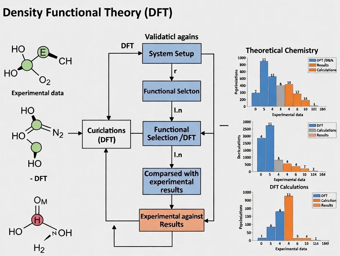
The following diagram illustrates the integrated computational-experimental workflow for DFT validation:

DFT Validation Workflow: Integrated computational and experimental approach.

Emerging approaches leverage artificial intelligence to automate and enhance DFT validation processes. The DREAMS framework exemplifies this trend with a multi-agent system for autonomous materials simulation:

AI-Enhanced DFT Framework: Multi-agent system for automated simulation.

Successful DFT validation requires access to specialized software tools, computational resources, and experimental databases. The following table catalogs essential resources for researchers conducting DFT validation studies:

Table 4: Essential Research Resources for DFT Validation

Resource Category	Specific Tools	Primary Function	Access Information
DFT Software [1]	VASP, Quantum Espresso, Gaussian, ORCA	Electronic structure calculation	Commercial licenses, free academic versions
Visualization Tools [1]	VESTA, Avogadro, GaussView	Structure modeling and result visualization	Free and commercial options
Experimental Databases [7]	JARVIS, Materials Project	Reference data for validation	Publicly accessible
Benchmark Datasets [4]	OMol25, Experimental redox data	Method validation and benchmarking	Publicly accessible
Computational Environments [1]	High-performance computing clusters, Cloud services	Execution of demanding calculations	Institutional resources, commercial cloud
Python Libraries [1]	PySCF, Psi4	Workflow integration and customization	Open source

The validation of DFT predictions against experimental data remains an essential process in computational chemistry and materials science. Based on the current analysis, several best practices emerge:

• Method Selection Should Match System Type: Traditional DFT functionals like B97-3c excel for main-group systems, while neural network potentials such as UMA-S show particular promise for organometallic complexes, especially for charge-related properties [4].

• Multiple Validation Properties Enhance Reliability: Successful validation studies typically compare computational predictions with multiple experimental observables (structural, electronic, magnetic, catalytic) to build comprehensive confidence in the computational models [2] [5].

• Integrated Workflows Improve Efficiency: Combining computational and experimental approaches from the initial research design phase creates a virtuous cycle of prediction, validation, and refinement that accelerates materials discovery and optimization [2] [5] [6].

• Emerging AI Technologies Show Promise: Frameworks like DREAMS demonstrate that AI-enhanced DFT approaches can achieve expert-level accuracy while reducing reliance on human intervention, potentially democratizing access to high-fidelity computational materials science [8].

As computational power increases and methodological innovations continue to emerge, the integration between DFT predictions and experimental validation will likely strengthen further. This synergy promises to accelerate the discovery and development of novel materials and pharmaceutical compounds while deepening our fundamental understanding of matter at the atomic scale.

Density Functional Theory (DFT) has become a cornerstone computational method across chemistry, materials science, and drug development. However, the predictive power of any DFT calculation depends critically on the chosen functional, basis set, and the specific physical properties being modeled. This guide provides an objective comparison of DFT performance against experimental data for three core physical properties: geometric structure, energy, and spectroscopic parameters. By synthesizing recent validation studies, we aim to equip researchers with practical benchmarks for selecting appropriate computational methods for their specific applications, from drug design to materials engineering.

The reliability of DFT predictions varies significantly across different molecular systems and properties. While some functionals excel at predicting molecular geometries, others may perform better for energy-related properties or spectroscopic simulations. This comparative analysis draws on direct experimental validation to highlight these performance differences, providing a framework for assessing computational results against empirical evidence across diverse chemical spaces.

Geometric Structure Validation

Performance Benchmarks for Molecular Systems

The accuracy of DFT in predicting molecular geometry is routinely validated against experimental X-ray crystallography data. Performance varies significantly across functionals and basis sets, with hybrid functionals generally providing superior agreement with experimental structures.

Table 1: Performance of DFT Functionals for Geometric Structure Prediction of Triclosan

Functional	Basis Set	Mean Absolute Error (Bond Lengths, Å)	Best Performing Bonds
M06-2X	6-311++G(d,p)	0.0353	C3-O10, O22-H23
CAM-B3LYP	LANL2DZ	0.0360	C12-C11, C3-C4
LSDA	LANL2DZ	0.0367	C12-Cl24, C6-Cl20
B3LYP	LANL2DZ	0.0453	-
PBEPBE	LANL2DZ	0.0514	-

In a comprehensive study of the triclosan molecule, the M06-2X functional coupled with the 6-311++G(d,p) basis set demonstrated superior performance in predicting bond lengths, achieving the lowest mean absolute deviation from experimental values (0.0353 Å) [9]. The CAM-B3LYP functional also performed well, particularly for predicting C12-C11 and C3-C4 bond distances [9]. The local spin-density approximation (LSDA) functional surprisingly outperformed B3LYP and PBEPBE for certain chlorine-containing bonds (C12-Cl24 and C6-Cl20), though it was less accurate for oxygen-hydrogen bonds [9].

For periodic systems like SiO₂ polymorphs, dispersion-corrected functionals are essential for accurate structure prediction. A broad assessment of 27 semi-local approaches found that the best-performing functionals achieved mean unsigned errors of approximately 0.2 T atoms per 1000 ų for framework densities when validated against experimental data [10].

Experimental Protocols for Geometric Validation

Standard experimental protocols for geometric validation typically involve single-crystal X-ray diffraction analysis. For the triclosan study, experimental molecular geometry parameters were obtained from crystallographic data and used as reference values for assessing computational predictions [9]. Similarly, structural validation of 5-(4-chlorophenyl)-2-amino-1,3,4-thiadiazole utilized single-crystal X-ray diffraction, with the compound crystallizing in the orthorhombic space group Pna2₁ with eight asymmetric molecules in the unit cell [11]. The experimental bond lengths and angles were directly compared with DFT-optimized geometries using root-mean-square deviation and mean absolute error as quantitative accuracy metrics.

Energy Property Validation

Reduction Potential and Electron Affinity Benchmarks

Energy-related properties such as reduction potentials and electron affinities present particular challenges for DFT methods due to their dependence on accurate electron correlation and charge distribution. Recent benchmarking studies reveal significant performance variations across computational methods.

Table 2: Performance of Computational Methods for Reduction Potential Prediction (Volts)

Method	System Type	Mean Absolute Error (V)	Root Mean Square Error (V)	R²
B97-3c	Main-group (OROP)	0.260	0.366	0.943
B97-3c	Organometallic (OMROP)	0.414	0.520	0.800
GFN2-xTB	Main-group (OROP)	0.303	0.407	0.940
GFN2-xTB	Organometallic (OMROP)	0.733	0.938	0.528
UMA-S (NNP)	Main-group (OROP)	0.261	0.596	0.878
UMA-S (NNP)	Organometallic (OMROP)	0.262	0.375	0.896

For reduction potential prediction, the B97-3c functional demonstrated strong performance for main-group species (MAE = 0.260 V) but showed reduced accuracy for organometallic systems (MAE = 0.414 V) [4]. Interestingly, the Universal Model for Atoms Small (UMA-S) neural network potential showed more consistent performance across both main-group and organometallic species, with MAEs of 0.261 V and 0.262 V respectively [4]. The semiempirical GFN2-xTB method performed reasonably for main-group molecules but exhibited significantly poorer accuracy for organometallic complexes (MAE = 0.733 V) [4].

For electron affinity calculations, the ωB97X-3c and r2SCAN-3c functionals generally provided the best agreement with experimental data for both main-group organic/inorganic species and organometallic coordination complexes [4]. These findings highlight the importance of method selection based on the specific chemical system under investigation.

Point Defect Formation Energy Validation

In materials science applications, predicting point defect formation energies represents another critical energy validation metric. Semi-local DFT functionals with a-posteriori corrections are often employed for high-throughput screening of defect properties, though their quantitative accuracy remains limited compared to hybrid functional approaches.

The formation energy for a charged defect Xᵩ is calculated as: Eᶠ(Xᵩ, εF) = Etot(Xᵩ) - Etot(bulk) - Σniμi + qεF + E_corr

where the correction term (E_corr) addresses spurious periodic image interactions and potential alignment issues [12]. Benchmarking against 245 "gold standard" hybrid calculations revealed that while semi-local DFT methods can provide useful qualitative trends for materials screening applications, their quantitative accuracy for defect transition levels and formation energies remains limited, particularly for systems with significant charge localization effects [12].

Experimental Protocols for Energy Validation

Experimental reduction potential values are typically determined through electrochemical measurements in appropriate solvent systems. The benchmarking study by Neugebauer et al. compiled experimental reduction potential data for 193 main-group species and 120 organometallic species, with geometries optimized using GFN2-xTB and solvent corrections applied using the Extended Conductor-like Polarizable Continuum Solvation Model (CPCM-X) [4].

For electron affinity validation, experimental gas-phase values were obtained from established literature for 37 simple main-group organic and inorganic species [4]. For organometallic systems, electron affinities were derived from experimental ionization energies of coordination complexes by reversing the sign of the reported values [4]. All DFT computations in these benchmark studies were conducted with strict convergence criteria, including a (99, 590) integration grid with robust pruning and an integral tolerance of 10⁻¹⁴ to ensure numerical accuracy [4].

Spectroscopic Parameter Validation

Vibrational Frequency Prediction

The accuracy of DFT in predicting vibrational frequencies is commonly assessed through comparison with experimental infrared and Raman spectroscopy data. Performance varies significantly with the choice of functional and basis set, with different combinations excelling for different molecular systems.

Table 3: Performance of DFT Methods for Vibrational Spectroscopy

System	Optimal Method	Key Metrics	Correlation with Experiment
Triclosan	LSDA/6-311G	Best vibrational frequency prediction	R² = 0.998 for 5-(4-chlorophenyl)-2-amino-1,3,4-thiadiazole
5-(4-chlorophenyl)-2-amino-1,3,4-thiadiazole	B3LYP/6-31+ G(d,p)	Vibrational frequencies	R² = 0.998
Graphene/GO	B3LYP/6-311 G	Longitudinal Optical mode	1585 cm⁻¹ (graphene), 1582 cm⁻¹ (graphene oxide)
Corannulene/Coronene	B3LYP/6-311 G	IR and Raman intensity	Aligns with theoretical predictions

For triclosan, the LSDA functional with the 6-311G basis set demonstrated superior performance in predicting vibrational spectra compared to other functionals, including hybrid methods [9]. The study employed the wavenumber-linear scaling (WLS) method to correct for the overestimation of calculated vibrational frequencies caused by neglect of anharmonicity effects and electron correlation [9].

For 5-(4-chlorophenyl)-2-amino-1,3,4-thiadiazole, DFT calculations at the B3LYP/6-31+ G(d,p) level showed excellent correlation with experimental vibrational frequencies (R² = 0.998) [11]. The B3LYP functional with the 6-311 G basis set also successfully predicted the Longitudinal Optical vibration mode in graphene-based systems, yielding values of 1585 cm⁻¹ for graphene and 1582 cm⁻¹ for graphene oxide that aligned well with theoretical predictions [13].

Electronic Spectroscopy and Properties

DFT calculations also facilitate the prediction of electronic spectroscopic properties, including UV-Vis absorption spectra and electronic transition energies. For 5-(4-chlorophenyl)-2-amino-1,3,4-thiadiazole, computational analysis revealed n→π* UV absorption characteristics and a significant first-order hyperpolarizability, suggesting potential applications in nonlinear optics [11].

The electronic properties of corannulene (C₂₀, C₂₀O) and coronene (C₂₄, C₂₄O) systems, including HOMO-LUMO energy levels and band gaps, have been successfully modeled using DFT with the 6-311 G basis set and B3LYP hybrid functional [13]. The calculated band gaps for corannulene (3.7 eV - 2.1 eV) and coronene (3.5 eV - 1.68 eV) provided insights into their electronic structures and reactivity [13].

Experimental Protocols for Spectroscopic Validation

Experimental vibrational validation typically employs Fourier-transform infrared (FT-IR) spectroscopy with samples prepared as KBr pellets for solid compounds [11]. Raman spectroscopy complements IR measurements, with spectra recorded across appropriate wavenumber ranges (e.g., 500-3500 cm⁻¹) [9]. For electronic spectroscopy, UV-Vis absorption spectra are measured in suitable solvents using spectrophotometers, with comparison to time-dependent DFT (TD-DFT) calculations for assignment of electronic transitions [11].

NMR spectroscopy provides additional validation through comparison of calculated chemical shifts with experimental ¹H and ¹³C NMR data [11]. High-resolution mass spectrometry (HRMS) serves to verify molecular ion peaks and confirm elemental compositions [11].

The Scientist's Toolkit: Essential Research Reagents and Materials

Table 4: Essential Research Reagents and Computational Tools for DFT Validation

Item	Function	Application Examples
Gaussian 09W/16	Quantum chemistry software package	Geometry optimization, frequency calculations [9]
CP2K	DFT code specializing in solid-state and periodic systems	SiO₂ polymorph studies, zeolite frameworks [10]
Quantum ESPRESSO	Open-source DFT package for periodic systems	Magnetic ferrite simulations [2]
GFN2-xTB	Semiempirical quantum mechanical method	Initial geometry optimization, conformer searching [4]
B3LYP functional	Hybrid density functional	General-purpose geometry and frequency calculations [11] [9]
M06-2X functional	Meta-hybrid density functional	Non-covalent interactions, precise geometry optimization [9]
6-311++G(d,p) basis set	Triple-zeta valence basis set with diffuse functions	Accurate geometry prediction for organic molecules [9]
def2-TZVPD basis set	Triple-zeta valence basis set	High-level reference calculations [4]
CPCM-X	Implicit solvation model	Solvent correction for reduction potential calculations [4]

This comparative analysis demonstrates that DFT validation against experimental data remains system- and property-dependent. For geometric structure prediction, the M06-2X/6-311++G(d,p) level consistently outperforms other functionals for organic molecules, while dispersion-corrected functionals are essential for periodic systems. For energy-related properties like reduction potentials, the B97-3c functional excels for main-group species, while neural network potentials like UMA-S show promising consistency across diverse chemical spaces. For spectroscopic validation, the optimal functional varies, with LSDA unexpectedly outperforming hybrid functionals for vibrational frequency prediction in some systems.

These findings underscore the importance of method validation for specific applications rather than relying on universal recommendations. Researchers should prioritize establishing validation protocols relevant to their target molecular systems and properties of interest. As computational methods continue to evolve, particularly with the emergence of machine-learning potentials, validation against robust experimental data will remain essential for ensuring predictive accuracy in drug development and materials design.

The validation of Density Functional Theory (DFT) against experimental crystallographic data represents a cornerstone of modern computational chemistry and materials science. This guide provides an objective comparison of various computational methods, with a specific focus on their performance in predicting molecular geometries and crystal packing, benchmarked against high-quality X-ray crystallographic data. The reliability of computational predictions is paramount for researchers in drug development and materials science, where in silico models are routinely used to predict molecular behavior, stability, and interactions before synthesis. We systematically evaluate the accuracy of multiple DFT functionals, semi-empirical methods, and machine learning potentials against experimental benchmarks for bond lengths, angles, and crystal packing arrangements, providing a clear framework for selecting appropriate computational tools based on specific research requirements.

Methodologies for Computational Validation

Experimental Crystallographic Benchmarking

The primary methodology for establishing ground-truth molecular geometries relies on single-crystal X-ray diffraction (SCXRD). This technique provides unambiguous three-dimensional structural information by measuring the diffraction pattern produced when X-rays interact with a crystalline sample [14]. The resulting electron density maps allow for precise determination of atomic positions, from which bond lengths, bond angles, and torsional angles can be derived with high accuracy. For organic compounds and small molecules, modern SCXRD can achieve precision in bond lengths of approximately 0.002 Å for non-hydrogen atoms [15], establishing it as the gold standard for structural validation.

When utilizing crystallographic data for benchmarking, several critical factors must be considered. The resolution of the diffraction data directly impacts model reliability, with higher resolution (typically <1.0 Å) providing greater atomic positioning accuracy [16]. Additionally, the completeness of the diffraction data and the clashscore of the refined model serve as important quality indicators. Researchers must also distinguish between equilibrium bond lengths (re) and vibrationally-averaged bond lengths (r0), as computational methods typically predict the former while experimental results from rotational spectra often provide the latter [17].

Computational Approaches for Geometry Prediction

Density Functional Theory (DFT) calculations represent the most widely used quantum mechanical approach for predicting molecular geometries. In a typical benchmarking study, computational methods are assessed by comparing predicted bond lengths, bond angles, and sometimes dihedral angles with their experimentally determined counterparts from crystallographic studies. The calculations involve geometry optimization of the target molecule, starting from either the experimental coordinates or a computationally generated structure, until a local energy minimum is located on the potential energy surface [15] [18].

For crystalline materials, more advanced approaches involve periodic DFT calculations that include the full crystal lattice parameters in the optimization process. This method allows for assessment of not only intramolecular geometry but also intermolecular interactions and crystal packing effects. In such cases, the root-mean-square Cartesian displacement (RMSD) between the experimental and optimized structures serves as a key metric, with values below 0.25 Å generally indicating correct structures [18].

Semi-empirical quantum mechanical methods such as GFN2-xTB offer a middle ground between accuracy and computational cost, enabling exhaustive conformational sampling of large molecular sets [19]. Recent advances also include machine learning potentials (MLPs) that can approach DFT-level accuracy at significantly reduced computational expense, making them increasingly valuable for crystal structure prediction [20].

Performance Comparison of Computational Methods

Accuracy in Bond Length Prediction

The performance of various computational methods was evaluated using creatininium cation structures as a benchmark system, with results compared against high-precision X-ray crystallographic data (Table 1) [15].

Table 1: Performance of Computational Methods for Bond Length Prediction

Method	Type	Mean Bond Length Error (Å)	Rank
MPW1B95	HMGGA	0.0126	1
PBEh	HGGA	0.0129	2
mPW1PW	HGGA	0.0133	3
SVWN5	LSDA	0.0142	4
B97-2	HGGA	0.0144	5
B3LYP	HGGA	0.0178	16
SCC-DFTB	SEMO	~0.03	>16

Note: HMGGA = Hybrid Meta Generalized Gradient Approximation; HGGA = Hybrid Generalized Gradient Approximation; LSDA = Local Spin Density Approximation; SEMO = Semiempirical Molecular Orbital

The data reveal significant variation in performance among DFT functionals, with the top-performing functionals (MPW1B95, PBEh, mPW1PW) achieving mean bond length errors of approximately 0.013 Å, approaching the experimental uncertainty of 0.002 Å [15]. Notably, the popular B3LYP functional performed less favorably with an error of 0.0178 Å, ranking 16th among the 21 tested functionals. Semi-empirical methods including SCC-DFTB demonstrated substantially larger errors, approximately 0.03 Å, highlighting the superior accuracy of DFT methods for geometric predictions [15].

Conformer Generation and Torsional Angle Prediction

Beyond bond lengths, the accurate prediction of molecular conformations and torsional preferences represents another critical benchmarking area. Large-scale studies comparing over 3 million compounds have revealed that quantum chemical methods like GFN2-xTB can generate conformer ensembles that closely match experimental crystallographic geometries, particularly for molecules with fewer rotatable bonds [19].

Table 2: Performance of Conformer Generation Methods

Method	Basis	RMSD for Small Molecules	RMSD for Protein Ligands
CREST/GFN2	Quantum	~0.2-0.5 Å (COD)	Higher RMSD (Platinum)
ETKDG	Crystallographic	Higher RMSD (COD)	Lower RMSD (Platinum)

For small molecules from the Crystallographic Open Database (COD), CREST/GFN2 ensembles demonstrated lower root-mean-square displacement (RMSD) values compared to the knowledge-based ETKDG method, particularly for molecules with zero to approximately 3-4 rotatable bonds [19]. This improved performance stems from better treatment of nonbonded interactions and electrostatics in the quantum mechanical method. However, for protein-bound ligands from the Platinum diverse set, ETKDG outperformed CREST/GFN2, suggesting that crystallographic data may better capture the extended conformations stabilized in binding sites [19].

Crystal Structure Prediction and Packing

The accurate prediction of complete crystal structures represents the most challenging benchmark, requiring correct reproduction of both molecular geometry and intermolecular packing. Recent evaluations of 13 state-of-the-art crystal structure prediction (CSP) algorithms revealed that performance remains far from satisfactory, with most algorithms struggling to identify correct space groups [20].

Machine learning potential-based CSP algorithms have achieved competitive performance compared to traditional DFT-based approaches, with success strongly dependent on the quality of the neural potentials and the global optimization algorithms employed [20]. For organic crystal structures, dispersion-corrected DFT (d-DFT) methods have demonstrated remarkable accuracy, with full energy minimization including unit-cell parameters producing average RMS Cartesian displacements of only 0.095 Å compared to experimental structures [18].

Figure 1: Workflow for Validating Computational Methods Against Crystallographic Data

Experimental Protocols

Crystallographic Data Collection and Processing

High-quality benchmarking requires meticulous attention to crystallographic data collection and processing protocols. Single crystals of suitable size and quality are mounted on diffractometers, and X-ray diffraction data are collected at appropriate temperatures (typically 100-293 K) [14]. The raw diffraction images are processed using specialized software to determine unit cell parameters and generate intensity data. Structure solution is typically achieved through direct methods or intrinsic phasing, followed by iterative least-squares refinement against F² values [14] [18].

Critical quality indicators must be monitored throughout this process, including data completeness, Rmerge, and the final R-factor values (Rwork and Rfree) [16]. For the deposited models of glutamate transporters, for instance, Rwork/Rfree values typically range from 21-30%, reflecting the moderate resolution (2.5-4.5 Å) of these membrane protein structures [16]. For small organic molecules, these values are generally significantly lower, reflecting higher precision.

Computational Benchmarking Procedures

Standardized computational protocols are essential for meaningful method comparisons. For molecular geometry assessments, researchers typically:

• Extract molecular structures from crystallographic data, removing solvent molecules and counterions if necessary [19]
• Perform geometry optimization using various computational methods, starting from the experimental coordinates [15]
• Calculate root-mean-square deviations (RMSD) between experimental and optimized structures [18]
• Statistically analyze differences in specific geometric parameters (bond lengths, angles, dihedrals) [15]

For crystal packing validation, more sophisticated approaches are required:

• Energy minimization of the complete crystal structure including unit cell parameters using dispersion-corrected DFT methods [18]
• Comparison of experimental and optimized structures using RMS Cartesian displacements [18]
• Analysis of intermolecular interactions and packing motifs before and after optimization [18]

RMSD values below 0.25 Å generally indicate correct structures, while higher values may signal problems with either the experimental model or the computational method [18].

The Scientist's Toolkit

Table 3: Essential Research Reagents and Resources

Resource	Type	Function	Example Sources
Crystallographic Databases	Data	Source of experimental reference structures	Crystallographic Open Database (COD), Cambridge Structural Database (CSD) [19]
Quantum Chemistry Software	Computational	Molecular geometry optimization	ORCA, Gaussian, CREST [19] [15]
DFT Functionals	Computational	Electron exchange-correlation approximation	MPW1B95, PBEh, B3LYP [15]
Semi-empirical Methods	Computational	Rapid conformational sampling	GFN2-xTB, AM1, PM3 [19] [15]
CSP Algorithms	Computational	Crystal structure prediction	CALYPSO, USPEX, GNOA [20]
Benchmark Platforms	Validation	Performance assessment of methods	CSPBench, CCCBDB [20] [17]

This comparison guide demonstrates that careful benchmarking against crystallographic data remains essential for validating computational methods in chemical research. DFT methods, particularly hybrid functionals like MPW1B95 and PBEh, provide excellent agreement with experimental bond lengths, with errors approaching experimental uncertainty. For conformational sampling, quantum chemical methods like GFN2-xTB outperform knowledge-based approaches for small molecules in the gas phase, while crystallography-derived methods maintain advantages for protein-bound ligands. In crystal structure prediction, machine learning potentials are achieving competitive performance with traditional DFT-based approaches, though significant challenges remain. Researchers should select computational methods based on their specific needs, considering the trade-offs between accuracy, computational cost, and applicability to their chemical systems of interest. As computational power increases and methods evolve, ongoing benchmarking against experimental crystallographic data will continue to be essential for methodological advancement and reliable application in drug development and materials design.

Density Functional Theory (DFT) has become an indispensable tool in computational chemistry, enabling the prediction of molecular properties by solving the fundamental equations of quantum mechanics. A critical validation of its performance lies in its ability to reproduce experimental spectroscopic data, particularly Nuclear Magnetic Resonance (NMR) parameters. This guide provides an objective comparison of DFT methodologies for predicting NMR chemical shifts and scalar coupling constants (J-couplings), benchmarking performance against experimental data and higher-level computational methods to establish reliability and identify limitations in the context of pharmaceutical and materials research.

Performance Comparison of DFT Methodologies

Accuracy of Chemical Shift Predictions

Extensive benchmarking studies have established the typical accuracy levels achievable with modern DFT approaches for predicting NMR chemical shifts. The table below summarizes the performance of various methodologies for a complex drug molecule, (R)-ispinesib, and small organic molecules.

Table 1: Accuracy of DFT for Predicting NMR Chemical Shifts in Drug Molecules and Small Organic Molecules

Method	Basis Set	Nucleus	Mean Absolute Error (MAE)	System Studied
O3LYP [21]	DGDZVP [21]	¹H	0.174 ppm [21]	(R)-ispinesib [21]
O3LYP [21]	DGDZVP [21]	¹³C	3.972 ppm [21]	(R)-ispinesib [21]
B3LYP [22]	6-31G(d) [22]	¹H	0.185 ppm [22]	Small Organic Molecules (NMRShiftDB2) [22]
B3LYP [22]	6-31G(d) [22]	¹³C	0.944 ppm [22]	Small Organic Molecules (NMRShiftDB2) [22]
B3LYP [22]	6-31G(d) [22]	¹H	0.078 ppm [22]	Small Organic Molecules (CHESHIRE) [22]
B3LYP [22]	6-31G(d) [22]	¹³C	0.504 ppm [22]	Small Organic Molecules (CHESHIRE) [22]
Not Specified [21]	6-31++G(d,p) [21]	¹H	~0.2 ppm [21]	Complex Drug Molecules [21]
Not Specified [21]	6-31++G(d,p) [21]	¹³C	<~6.0 ppm [21]	Complex Drug Molecules [21]

The data demonstrates that DFT can achieve high accuracy for ¹H chemical shifts, with MAE values often below 0.2 ppm, which is sufficient for distinguishing between many different chemical environments [21]. For ¹³C nuclei, errors are larger but remain chemically insightful, typically under 6 ppm for complex drug molecules and below 1 ppm for optimized small molecule datasets [22] [21]. The choice of basis set is crucial, with double-ζ basis sets like DGDZVP and 6-31++G(d,p) often providing an optimal balance of accuracy and computational cost, sometimes outperforming larger triple-ζ sets [21].

Accuracy of Scalar Coupling Constant (J) Predictions

The prediction of scalar coupling constants presents a greater challenge for DFT than chemical shifts. J-couplings, especially the dominant Fermi contact term, are highly sensitive to the electron density at the nucleus, requiring high-quality wavefunctions [23].

Table 2: Performance of Computational Methods for Scalar Coupling Constants

Method	Type of Coupling	Performance / Key Findings
DFT (General) [23]	Multiple types (¹J, ²J, ³J)	More demanding than chemical shift calculations due to sensitivity to wavefunction near the nucleus [23].
Graph Angle-Attention Neural Network (GAANN) [24]	Multiple types (¹J, ²J, ³J)	Prediction accuracy log(MAE) = -2.52, close to DFT accuracy but much faster [24].
DFT for Enantiospecificity	J-couplings between enantiomers	Fails to explain reported enantiospecific NMR responses; differences between enantiomers are negligible and attributable to numerical noise [25].
DFT/FPT (B3PW91/6-311G) [26]	Hydrogen-bond couplings (e.g., ( ^h2J_{N-H...N} ))	Can successfully calculate J-couplings through hydrogen bonds and correlate them with H-bond distances [26].

A significant finding from recent research is that standard DFT calculations are parity-conserving, meaning they predict identical J-couplings for two enantiomers (mirror-image molecules) [25]. Reported enantiospecific differences in cross-polarization NMR experiments are likely due to variations in sample conditions (purity, crystallinity) rather than calculable differences in J-couplings themselves [25]. For standard applications, machine learning models like the Graph Angle-Attention Neural Network (GAANN) now offer accuracy close to DFT calculations at a fraction of the computational cost, highlighting a growing trend in the field [24].

Experimental and Computational Protocols

Standard Protocol for Chemical Shift Calculation

A robust workflow for calculating NMR chemical shifts involves multiple steps to ensure accuracy and reliability, from initial structure generation to final calculation.

Diagram 1: Chemical shift calculation workflow.

1. Initial Structure and Conformer Generation: The process begins with a 2D molecular representation (e.g., SMILES or InChI). For flexible molecules, multiple low-energy 3D conformers are generated using algorithms like ETKDG and force fields like MMFF94 [22] [27]. The lowest-energy conformer is typically selected, or chemical shifts are Boltzmann-averaged across several low-energy conformers [27].

2. Geometry Optimization: This is a critical step. The initial 3D structure must be optimized using DFT to locate a true energy minimum. Complete geometry optimization is essential for achieving the highest accuracy in both ¹H and ¹³C chemical shifts [21]. This can be performed in the gas phase or, more accurately, using an implicit solvation model (e.g., PCM, SMD, or COSMO) to mimic the experimental solvent environment [21] [27].

3. NMR Calculation with GIAO: The chemical shielding tensor (σ) is calculated for the optimized geometry using the Gauge-Including Atomic Orbital (GIAO) method, which ensures results are independent of the coordinate system origin [21] [28]. This calculation is performed at a consistent level of theory (functional and basis set).

4. Referencing and Linear Regression: The isotropic shielding constant (σi) for each nucleus is converted to a chemical shift (δi) by referencing against a standard like tetramethylsilane (TMS): δi = σref - σi + δref, where δ_ref for TMS is 0 ppm [27]. For greater accuracy, empirical linear regression (scaling) between calculated shieldings and experimental shifts of a training set is often applied [22].

Protocol for Scalar Coupling Constants

The calculation of J-couplings is more specialized. The Fermi contact (FC) term is usually dominant and requires a high-quality basis set capable of describing the wavefunction correctly at the atomic nucleus [23]. The finite perturbation theory (FPT) approach is commonly used within DFT frameworks [26] [23]. As with chemical shifts, using a well-optimized geometry is paramount. It is critical to use identical, mirror-image conformations when comparing enantiomers, as conformational differences (e.g., dihedral angles) can induce large apparent variations in J-couplings via the Karplus relationship, which are easily mistaken for genuine enantiospecific effects [25].

The Scientist's Toolkit: Essential Research Reagents & Materials

Table 3: Key Software, Functionals, and Basis Sets for DFT-NMR Validation

Tool Name	Type	Primary Function & Application Notes
Gaussian [21]	Software Suite	Industry-standard software for quantum chemistry calculations, widely used for NMR parameter prediction via GIAO [21].
ORCA [25]	Software Suite	Open-source quantum chemistry package featuring advanced methods (e.g., X2C) for relativistic NMR calculations [25].
NWChem [27]	Software Suite	High-performance computational chemistry software used for automating chemical shift calculations on large molecule sets [27].
B3LYP [22] [21]	Hybrid Functional	The dominant hybrid functional for NMR calculations, offering a reliable balance of accuracy for various systems [22] [21].
PBE0/BP86 [29]	Functional	Popular GGA functionals (BP86) and their hybrid variants (PBE0) often used for geometry optimization and property calculations [29].
6-31G(d) / 6-31++G(d,p) [21]	Basis Set	Pople-style basis sets; double-ζ with polarization and diffuse functions offer a good cost-accuracy balance for NMR [21].
def2-TZVP [25]	Basis Set	Ahlrichs-style triple-ζ basis set with polarization, used for higher-accuracy calculations [25].
DGDZVP [21]	Basis Set	Double-ζ basis set specifically developed for DFT, often excellent for NMR chemical shift prediction [21].
IGLO-III [23]	Basis Set	Historically significant basis set designed for NMR property calculations (IGLO = Individual Gauge for Localized Orbitals) [23].

DFT has matured into a highly reliable tool for predicting NMR chemical shifts, with accuracy often sufficient to guide structural assignment and elucidation in complex drug molecules and organic compounds. Its performance for scalar coupling constants is more nuanced; while it successfully predicts J-couplings in hydrogen-bonded systems and for conformational analysis, it cannot explain purported enantiospecific couplings, a limitation rooted in its parity-conserving nature. The synergy between experimental NMR spectroscopy and DFT calculations, when protocols are carefully followed, provides a powerful framework for validating molecular structures, with emerging machine learning methods offering a promising path for rapid, large-scale predictions.

The Critical Role of Validated Datasets for Method Development and Benchmarking

Density Functional Theory (DFT) serves as the workhorse of modern quantum mechanics calculations for molecular and periodic structures, yet its predictive reliability depends critically on the quality of validation against experimental data. Despite countless studies demonstrating DFT's accuracy across various systems, few have comprehensively targeted industrially-relevant materials or provided clear guidance on functional selection, expected deviation from experimental values, or pseudopotential performance [30]. This validation gap becomes particularly problematic as researchers increasingly rely on computational data to train machine learning interatomic potentials (MLIPs), where errors in underlying DFT calculations propagate and potentially amplify through trained models. The foundational question remains: how can practitioners distinguish between methodological limitations and numerical errors in their computational workflows?

The emergence of large-scale DFT datasets has attempted to address this challenge, but recent investigations reveal surprising inconsistencies in even widely-used benchmark data. This analysis examines the critical importance of validated datasets for robust method development and benchmarking in computational chemistry, providing a structured comparison of available resources and their experimental validation status to guide researchers in selecting appropriate datasets for their specific applications.

The Current Landscape of DFT Datasets

The proliferation of DFT datasets has created both opportunities and challenges for computational chemists. These datasets vary dramatically in chemical diversity, numerical quality, and experimental validation, factors that directly impact their utility for method development and benchmarking.

Table 1: Key Characteristics of Major Molecular DFT Datasets

Dataset	Size (Configurations)	Level of Theory	Chemical Diversity	Reported Validation
OMol25 [31]	100 million	ωB97M-V/def2-TZVPD	83 elements (H-Bi); biomolecules, metal complexes, electrolytes	Extensive baseline MLIP benchmarks; internal consistency checks
ANI-1x [32]	5.0 million (6-31G*), 4.6 million (def2-TZVPP)	ωB97x/6-31G* and ωB97x/def2-TZVPP	Organic molecules and drug-like compounds	Comparison between basis sets; limited experimental validation
SPICE [32]	2.0 million	ωB97M-D3(BJ)/def2-TZVPPD	Small molecules and peptides	Intended for biomolecular force field development
ANI-1xbb [32]	13.1 million	B97-3c	Diverse organic molecules	Focus on broad coverage rather than high accuracy
QCML [32]	33.5 million	PBE0	Focused chemical space	High-throughput screening oriented
Transition1x [32]	9.6 million	ωB97x/6-31G(d)	Reaction transition states	Chemical reaction benchmarking

Recent analyses have uncovered significant quality concerns in several popular datasets. A 2025 study examining net forces in DFT datasets found that the ANI-1x, Transition1x, AIMNet2, and SPICE datasets contain unexpectedly large nonzero net forces, indicating suboptimal DFT settings and numerical errors [32]. These force inaccuracies averaged from 1.7 meV/Å in the SPICE dataset to 33.2 meV/Å in the ANI-1x dataset when compared to recomputed forces using more reliable DFT settings at the same level of theory [32]. Such errors are particularly concerning given that general-purpose MLIP force mean absolute errors are now approaching 10 meV/Å, meaning that errors in training data may fundamentally limit model accuracy.

Diagram 1: The dataset development and validation workflow. The red node highlights quality control as a critical checkpoint, while green indicates experimental validation - the essential step often minimized in practice.

Case Studies: Dataset Validation in Practice

OMol25: A High-Precision Benchmark

The OMol25 dataset represents a significant advancement in dataset quality, incorporating rigorous quality control measures and extensive chemical diversity. With over 100 million calculations at the ωB97M-V/def2-TZVPD level, OMol25 spans 83 elements (H through Bi) and includes biomolecules, metal complexes, and electrolytes [31]. The dataset implements stringent numerical precision protocols, including the DEFGRID3 setting in ORCA 6.0.0 with 590 angular points for exchange-correlation and 302 for COSX, specifically designed to mitigate numerical noise between energy gradients and forces [31]. This attention to numerical detail results in negligible net forces throughout the dataset, addressing a key limitation of earlier resources.

OMol25's validation approach includes comprehensive baseline evaluations using state-of-the-art equivariant graph neural network architectures (eSEN, GemNet-OC, MACE) with explicit reporting of out-of-distribution test errors [31]. The dataset also includes specialized benchmarking tasks such as conformer ensemble ranking, protein-ligand interaction energies, and spin-gap calculations, providing multifaceted validation metrics beyond simple energy comparisons.

Experimental Validation in Materials Science

The National Institute of Standards and Technology (NIST) addresses DFT validation through targeted studies on industrially-relevant material systems [30]. Their work focuses on three critical domains: pure and alloy solids for CALPHAD method development, metal-organic frameworks (MOFs) for carbon capture applications, and metallic nanoparticles for catalytic applications. In each domain, systematic comparisons between different functionals, pseudopotentials, and basis sets provide practical guidance for method selection.

A particularly insightful finding from NIST's work concerns the sensitivity of MOF adsorption properties to the choice of partial charge calculation scheme [30]. Despite using identical DFT methodologies, different charge derivation approaches produced significantly different equilibrium properties for MOF-adsorbate systems, highlighting how methodological choices beyond the core DFT calculation can impact predictive accuracy and experimental agreement.

Machine Learning Correction of DFT Errors

A 2025 study demonstrated a machine learning approach to correct systematic errors in DFT-calculated formation enthalpies for alloys [33]. By training neural network models on the discrepancy between DFT-calculated and experimentally measured enthalpies for binary and ternary alloys, researchers achieved significant improvements in phase stability predictions. The model utilized structured feature sets including elemental concentrations, atomic numbers, and interaction terms to capture key chemical effects, then applied these corrections to the Al-Ni-Pd and Al-Ni-Ti systems relevant for high-temperature aerospace applications [33].

This approach highlights a pragmatic middle ground: rather than seeking perfect DFT functionals, researchers can develop targeted error correction models trained on well-validated experimental data, effectively bridging the accuracy gap for specific applications.

Quantitative Benchmarking of Computational Methods

Recent comparative studies provide valuable insights into the relative performance of different computational methods when validated against experimental data.

Table 2: Method Performance on Experimental Reduction Potentials (Mean Absolute Error in V) [4]

Method	Main-Group Species (OROP)	Organometallic Species (OMROP)	Validation Approach
B97-3c	0.260	0.414	Experimental reduction potentials in solvent
GFN2-xTB	0.303	0.733	Experimental reduction potentials in solvent
eSEN-S (OMol25)	0.505	0.312	Experimental reduction potentials in solvent
UMA-S (OMol25)	0.261	0.262	Experimental reduction potentials in solvent
UMA-M (OMol25)	0.407	0.365	Experimental reduction potentials in solvent

The benchmarking results reveal several noteworthy patterns. First, the performance of methods varies significantly between main-group and organometallic species, highlighting the domain dependence of computational accuracy [4]. Surprisingly, certain neural network potentials (UMA-S) achieved accuracy comparable to or better than traditional DFT for organometallic systems despite not explicitly incorporating charge-based physics in their architecture. Second, method performance is not necessarily correlated with computational cost, with the smaller UMA-S model outperforming the larger UMA-M model on both chemical domains [4].

For electron affinity predictions, the same study found that OMol25-trained NNPs performed comparably to low-cost DFT and semiempirical quantum mechanical methods for main-group species but showed advantages for organometallic complexes, suggesting that data-driven approaches may offer particular benefits for chemically complex systems [4].

Experimental Protocols for DFT Validation

Force Validation Protocol

The 2025 force accuracy study established a rigorous protocol for validating DFT forces [32]:

• Sample Selection: Randomly select 1000 configurations from the target dataset
• Reference Computation: Recompute forces using the same functional and basis set but with tighter numerical settings
• Error Metric Calculation: Compute root mean square errors (RMSE) for force components
• Net Force Analysis: Calculate the magnitude of net forces per atom as an initial error indicator

This protocol identified that disabling the RIJCOSX approximation in older ORCA versions eliminated significant net forces in several datasets, providing both a specific remediation for existing data and a warning for future dataset generation [32].

Thermodynamic Property Validation

The ML correction study for formation enthalpies implemented this validation workflow [33]:

• Data Curation: Filter experimental formation enthalpies to exclude unreliable values
• Feature Engineering: Create structured input features including elemental concentrations, weighted atomic numbers, and interaction terms
• Model Training: Train neural network regressors to predict DFT-experiment discrepancies
• Cross-Validation: Apply leave-one-out and k-fold cross-validation to prevent overfitting
• Application: Apply corrected enthalpies to phase diagram calculations

This approach demonstrated that ML corrections could significantly improve predictive accuracy for ternary phase stability while maintaining computational efficiency [33].

Essential Research Reagents and Computational Tools

Table 3: Key Computational Tools for DFT Validation

Tool/Resource	Function	Application in Validation
Quantum ESPRESSO [34]	Plane-wave DFT code	Electronic structure, mechanical properties
ORCA [32]	Quantum chemistry package	Molecular DFT with various functionals
NIST CCCBDB [30]	Computational chemistry database	Experimental comparison data
DFT Material Properties Simulator [34]	Web-based simulation tool	Educational validation exercises
MSR-ACC/TAE25 [35]	Accurate thermochemistry dataset	High-level reference data

The selection of appropriate computational tools significantly impacts validation outcomes. For example, the DFT Material Properties Simulator provides an accessible platform for novice users to compute electronic band structures, density of states, and mechanical properties while maintaining advanced options for experienced researchers [34]. Such tools lower the barrier to entry for DFT validation while maintaining methodological rigor.

Future Directions and Recommendations

The evolving landscape of DFT validation suggests several critical directions for future development:

• Standardized Validation Metrics: The field would benefit from community-agreed standards for dataset quality metrics, particularly for force accuracy, energy consistency, and experimental agreement.

• Specialized Benchmark Sets: Rather than universal datasets, purpose-built benchmark sets for specific chemical domains (organometallics, biomolecules, materials interfaces) would provide more targeted validation.

• ML-Augmented Validation: Machine learning approaches show promise for both error correction and quality assessment, potentially identifying problematic calculations before they enter training datasets.

• Transparent Reporting: Dataset creators should provide comprehensive documentation of numerical settings, convergence criteria, and known limitations to enable appropriate use.

• Experimental Collaboration: Stronger partnerships between computational and experimental groups would ensure validation against reliable, well-characterized reference data.

As dataset size and diversity continue to expand, the critical role of rigorous validation against experimental data becomes increasingly important. By adopting the protocols, metrics, and resources outlined here, researchers can make informed decisions about dataset selection and method development, ultimately enhancing the predictive reliability of computational chemistry across scientific and industrial applications.

Computational Protocols and Applications: Achieving Accurate DFT Results for Biomolecules and Materials

Density Functional Theory (DFT) has become an indispensable computational tool for researchers investigating molecular and material properties across chemical, biological, and physical sciences. The practical application of DFT requires careful selection of two fundamental components: the exchange-correlation functional and the atomic basis set. These choices create a complex landscape where accuracy, computational cost, and applicability to specific chemical systems are often in direct competition. The proliferation of available functionals and basis sets necessitates evidence-based protocols to guide researchers in selecting optimal combinations for their specific tasks. This guide provides a comparative analysis of contemporary DFT approaches, validating methodologies against experimental data to establish robust protocols for diverse research applications in drug development and materials science.

Table 1: Common Basis Set Families and Their Characteristics

Basis Set Family	Key Examples	General Characteristics	Recommended Use Cases
Pople	6-31G(d), 6-311+G(d,p) [36]	Split-valence, widely used, good balance of speed/accuracy [37]	General organic molecules; 6-31G(d) is a common default [37]
Dunning's cc-pVXZ	cc-pVDZ, cc-pVTZ, cc-pVQZ [36]	Correlation-consistent, systematic convergence to complete basis set limit [36]	High-accuracy post-Hartree-Fock and DFT calculations [37]
Ahlrichs/Karlsruhe (def2)	def2-SVP, def2-TZVP, def2-QZVP [36] [38]	Balanced performance, widely used in modern composite methods [36]	General-purpose DFT, especially with transition metals [36]
Jensen (pcseg)	pcseg-1, pcseg-2, aug-pcseg-2 [37]	Polarization-consistent, often outperform Pople sets at similar cost [37]	Highly recommended for DFT calculations [37]
Specialized (vDZP)	vDZP [38]	Recently developed, minimizes basis set superposition error (BSSE) [38]	Efficient, low-cost calculations with various functionals [38]

Comparative Analysis of Density Functionals

The Benchmarking Landscape and Functional Performance

The development of robust DFT protocols relies on comprehensive benchmarking against reliable experimental data and high-level theoretical references. The GMTKN55 database, an expansive collection of main-group thermochemistry benchmarks, has become a standard for quantifying functional accuracy [38]. Performance on such benchmarks reveals that no single functional excels universally, but their strengths and weaknesses can be mapped to specific chemical properties and systems.

The ubiquitous B3LYP functional serves as a common starting point in many studies. However, benchmarks show it has specific limitations: it performs reasonably well for basic properties and barrier heights but is "one of the worst overall for reaction energies" and can over-stabilize high-spin states in open-shell 3d transition metal complexes [39]. Its performance improves significantly when augmented with an empirical dispersion correction, such as D3(BJ) [39]. Modern functionals like ωB97X-D, PW6B95, and M06-2X often outperform B3LYP across broader benchmark sets [39]. The machine-learning-aided development of functionals is an emerging frontier, showing promise for creating more universal exchange-correlation approximations trained on high-quality quantum data [40].

Task-Specific Functional Recommendations

• Reaction Energies and Thermochemistry: Functionals like PW6B95 and double-hybrid functionals (e.g., DSD-BLYP) generally show superior performance for reaction energies and isomerizations [39]. B3LYP is not recommended for this domain due to its high errors [39].
• Non-Covalent Interactions: Accurate modeling of dispersion forces (London dispersion, π-π stacking) requires functionals with built-in dispersion corrections or the explicit addition of empirical corrections like D3(BJ) or D4 [39] [38]. The ωB97X-D functional is a strong performer in this category [39].
• Transition Metal Chemistry: Standard hybrid functionals like B3LYP are known to over-stabilize high-spin states. Using a modified version with 15% Hartree-Fock exchange (B3LYP*) or opting for functionals like TPSSh can mitigate this issue [39].
• Band Structures and Solid-State Properties: For periodic systems, meta-GGAs like SCAN and r²SCAN offer a good balance of accuracy and cost, often outperforming GGAs and hybrids for bulk properties [38].

Basis Set Selection Strategies

Basis Set Types and Systematic Convergence

Basis sets expand molecular orbitals as linear combinations of atom-centered functions, with quality increasing with the number of functions per atom (ζ-level). Minimal basis sets (e.g., STO-3G) provide the most computationally economical description but suffer from significant incompleteness error [38]. Double-ζ basis sets (e.g., 6-31G(d), def2-SVP, pcseg-1) offer a better balance and are common for geometry optimizations and frequency calculations [37]. For higher accuracy, triple-ζ basis sets (e.g., 6-311+G(d,p), def2-TZVP, cc-pVTZ) provide results closer to the complete basis set limit but at a substantially higher computational cost—often more than five-fold slower than double-ζ sets [38].

The recent vDZP basis set demonstrates that specialized double-ζ sets can achieve accuracy approaching that of conventional triple-ζ basis sets. In benchmarks, vDZP combined with various functionals (B3LYP-D4, M06-2X, B97-D3BJ, r²SCAN-D4) yielded results "only moderately worse" than the much larger (aug)-def2-QZVP basis set, making it a highly efficient choice for a wide range of functionals without need for reparameterization [38].

Practical Basis Set Recommendations

• Geometry Optimizations and Frequency Calculations: Double-ζ basis sets with polarization functions, such as 6-31G(d) (also called 6-31G*), def2-SVP, or the highly recommended pcseg-1, offer a good compromise between cost and accuracy [37].
• Accurate Energy Calculations (Single-Points): For final energy evaluations on pre-optimized structures, use larger triple-ζ basis sets like 6-311+G(d,p), def2-TZVP, or cc-pVTZ(seg-opt) [37]. The "seg-opt" variant of Dunning's basis sets is recommended for improved computational efficiency [37].
• Non-Covalent Interactions and Anionic Systems: Include diffuse functions (e.g., 6-311++G(d,p), aug-cc-pVDZ) to properly describe electron densities far from the nucleus [36] [37].
• High-Throughput and Large Systems: The vDZP basis set or polarized minimal basis sets like MIDI! provide maximum speed while retaining useful accuracy [37] [38].

Table 2: Functional/Basis Set Performance on GMTKN55 Benchmark (Weighted Total Mean Absolute Deviation (WTMAD2) in kcal/mol) [38]

Functional	Large Quadruple-ζ Basis Set	vDZP Basis Set	Performance Gap
B97-D3BJ	8.42 (def2-QZVP)	9.56	+1.14
r²SCAN-D4	7.45 (def2-QZVP)	8.34	+0.89
B3LYP-D4	6.42 (def2-QZVP)	7.87	+1.45
M06-2X	5.68 (def2-QZVP)	7.13	+1.45
ωB97X-D4	3.73 (def2-QZVP)	5.57	+1.84

Experimentally Validated Case Study: Dopamine Sensing with CuO–ZnO Nanocomposites

Experimental Protocol and Methodology

A practical example integrating DFT with experimental validation involves developing a high-sensitivity sensor for the neurotransmitter dopamine (DA) using CuO–ZnO nanocomposites [41]. Researchers synthesized four distinct CuO–ZnO composites via a one-step hydrothermal method by varying the mass fraction of CuCl₂ precursor (1%, 3%, 5%, 7%) [41]. The composite formed with 3% CuCl₂ developed a unique nanoflower morphology composed of intersecting nanorods, which exhibited superior catalytic performance [41].

DFT simulations revealed the origin of this enhanced activity: the CuO–ZnO nanoflower structure reduced the reaction energy barrier for dopamine oxidation to 0.54 eV and modified the electronic structure (projected density of states), bringing the d-band center of Cu closer to the Fermi level [41]. This theoretical insight guided the construction of an electrochemical sensor, which demonstrated a remarkably low detection limit (LOD) of 6.3 nM for dopamine and high sensitivity (34467.3 µA·(mM)⁻¹·cm⁻²) in biological fluids like human serum and urine [41]. The close correlation between predicted catalytic enhancement and experimental performance validates the DFT model's predictive power for materials design.

Table 3: Key Research Reagent Solutions for Electrochemical Sensor Development [41]

Material/Reagent	Function/Role in Experiment
ZnCl₂	Primary zinc precursor for ZnO formation in hydrothermal synthesis
CuCl₂	Copper dopant precursor; concentration variation (1-7 wt%) controls composite morphology
NaOH	Hydroxide source for metal oxide precipitation and crystal growth
PEG-400/Water Solution	Solvent medium (1:1 v/v) for hydrothermal synthesis; PEG acts as a stabilizing agent
Dopamine (DA)	Target analyte for electrochemical sensing and catalytic performance validation
Human Serum and Urine	Complex biological matrices for validating sensor practicality and selectivity

Integrated Protocols for Robust Computational Chemistry

Consolidated Best-Practice Recommendations

• Define the Objective First: Select the functional and basis set based on the target property (e.g., reaction energy, geometry, non-covalent interaction). Avoid using a single combination for all problems.
• Employ a Multi-Level Approach: Optimize molecular geometries with a moderate-cost method (e.g., B3LYP-D3(BJ)/def2-SVP or pcseg-1) then perform single-point energy calculations with a higher-level method (e.g., DSD-BLYP/def2-TZVP or ωB97X-D/cc-pVTZ) on the optimized structure.
• Always Include Dispersion Corrections: For most modern functionals, add an empirical dispersion correction (e.g., D3(BJ) or D4), as it dramatically improves the description of non-covalent interactions at negligible computational cost [39] [38].
• Validate with Composite Methods: For non-specialists, established composite methods (e.g., B97-3c, ωB97X-3c, r²SCAN-3c) provide robust, well-balanced performance as they integrate a pre-defined functional, basis set, and empirical corrections [38].
• Benchmark Where Possible: For systems with known experimental data or high-level theoretical references, conduct a limited benchmark of 2-3 functionals to identify the best-performing one for your specific chemical system.

Future Directions in DFT Development

The field of DFT continues to evolve rapidly. Key trends include the rise of machine-learned functionals, which are trained on high-quality quantum data to discover more universal exchange-correlation approximations while keeping computational costs low [40]. The development of novel, efficient basis sets like vDZP that minimize BSSE and approach triple-ζ accuracy at double-ζ cost is also progressing [38]. Furthermore, the increased integration of DFT with molecular dynamics (DFT-MD) allows for the simulation of materials and chemical processes under realistic conditions, as demonstrated in studies of graphene-CO₂ interactions [6]. These advancements promise to further narrow the gap between computational prediction and experimental reality, solidifying DFT's role as a cornerstone of modern molecular research and drug development.

Density Functional Theory (DFT) has become the most widely utilized first-principles method for theoretically modeling materials at the electronic level because it provides a reasonable balance between accuracy and computational cost [42]. Within the Kohn-Sham approach to DFT, the most complex electron interactions are collected into an exchange-correlation (XC) energy functional (E({}_{xc})), whose exact form remains unknown and must be approximated [42]. The accuracy of DFT predictions therefore hinges upon the choice of XC functional used to model electron-electron interactions [42] [43].

Perdew and coworkers proposed an illustrative hierarchy known as Jacob's ladder, which classifies XC functionals in ascending order of theoretical rigor and complexity [42]. This ladder provides a framework for understanding the relationships between different functional types:

• Local Density Approximation (LDA): Occupies the first rung, depending only on the electron density ρ
• Generalized Gradient Approximation (GGA): The second rung incorporates both ρ and its gradient ∇ρ
• Meta-GGA: The third rung adds dependency on the orbital kinetic energy density τ
• Hybrid functionals: The fourth rung incorporates a fraction of exact Hartree-Fock exchange
• Double hybrids: The fifth rung includes both Hartree-Fock exchange and perturbative correlation

This guide focuses on three foundational functionals from the lower rungs of this ladder—LDA, PBE (GGA), and B3LYP (hybrid)—comparing their theoretical formulations, performance characteristics, and practical applications across diverse material systems.

Theoretical Foundations: Functional Formulations and Implementations

Mathematical Frameworks and Functional Forms

The Local Density Approximation (LDA) represents the simplest functional form, with the exchange-correlation energy depending only on the electron density ρ at each point in space [44]. Common implementations include the VWN (Vosko-Wilk-Nusair) functional, which parametrizes electron gas data, and the PW92 (Perdew-Wang 1992) functional [44]. The fundamental limitation of LDA stems from its neglect of electron density inhomogeneity.

The PBE (Perdew-Burke-Ernzerhof) functional exemplifies the Generalized Gradient Approximation (GGA) approach, incorporating both the electron density ρ and its gradient ∇ρ to account for inhomogeneities in electron distribution [42] [44]. This functional was constructed to satisfy specific physical constraints without empirical parameters [44].

B3LYP (Becke, 3-parameter, Lee-Yang-Parr) represents a hybrid functional that mixes the Hartree-Fock exact exchange with GGA exchange and correlation [45]. The functional takes the form:

[ E{xc}^{B3LYP} = aEx^{HF} + (1-a)Ex^{LDA} + b\Delta Ex^{B88} + Ec^{LDA} + c\Delta Ec^{LYP} ]

where a, b, c are empirical parameters (a = 0.20, b = 0.72, c = 0.81) determined by fitting to experimental data [45]. This combination of exact exchange with DFT approximations improves the treatment of many electronic properties but increases computational cost substantially.

Table 1: Theoretical Specifications of Core Exchange-Correlation Functionals

Functional	Type	Exchange Component	Correlation Component	HF Exchange	Theoretical Approach
LDA (VWN)	Local	Slater/Dira	VWN	0%	Homogeneous electron gas
PBE	GGA	PBEx	PBEc	0%	Constraint satisfaction
B3LYP	Hybrid	Becke88 (B88)	LYP	20%	Empirical parameter mixing

Computational Implementation Considerations

Implementing these functionals requires careful consideration of several computational factors. The projector augmented-wave (PAW) method and pseudopotentials are commonly employed to treat core electrons efficiently, particularly for systems containing heavy elements [42]. For materials with strong relativistic effects, such as those containing rare-earth elements, spin-orbit coupling (SOC) corrections become necessary for qualitatively accurate electronic descriptions [42].

The basis set selection critically influences computational accuracy and cost. For molecular systems, polarized basis sets with diffuse functions (e.g., aug-cc-pVDZ, def2-TZVP) are essential for properties like polarizabilities [46] [47]. Periodic systems typically employ plane-wave basis sets with kinetic energy cutoffs.

Figure 1: Jacob's Ladder of DFT Functionals showing the ascending hierarchy of exchange-correlation approximations with increasing complexity and theoretical rigor [42]

Performance Comparison Across Material Systems

Solid-State Materials and Rare-Earth Oxides

For solid-state systems, the choice of functional significantly impacts the accuracy of predicting structural, electronic, and magnetic properties. A comprehensive benchmarking study assessing 13 different DFT functionals for rare-earth oxides (REOs) revealed that meta-GGA functionals, particularly the r2SCAN functional, delivered high accuracy for structural, electronic, and energetic predictions [42]. The study highlighted that +U corrections (DFT+U) are critical for accurate REO electronic structure modeling to address self-interaction errors in localized 4f electrons [42].

In magnetic materials like L1₀-MnAl compounds, GGA functionals (PBE) provide greater accuracy in describing electronic structure and magnetic behavior compared to LDA [43]. LDA tends to underestimate lattice parameters, while GGA shows better agreement with experimental values [43]. Specifically, for L1₀-MnAl, GGA predicted a magnetic moment of 2.45 μB, closer to experimental observations than LDA's prediction of 2.20 μB [43].

Table 2: Functional Performance for Solid-State Properties

Material System	LDA Performance	PBE/GGA Performance	B3LYP/Hybrid Performance	Recommended Functional
Rare-earth oxides	Poor for electronic structure due to strong correlation	Moderate, requires +U correction for 4f electrons	Good but computationally expensive	r2SCAN+U or SCAN+U [42]
Magnetic materials (L1₀-MnAl)	Underestimates lattice parameters, magnetic moments	Good structural and magnetic accuracy	Limited data for metallic systems	PBE [43]
General solids	Overbinding, underestimated lattice constants	Reasonable lattice parameters	Good but high computational cost	PBE or PBEsol [42]
Band gaps	Severe underestimation	Moderate underestimation	Improved but still underestimated	HSE06 or other range-separated hybrids

Molecular Systems and Biological Applications

For molecular systems, benchmark studies using adaptive force matching (AFM) provide insights into functional performance for conformational distributions and free energy profiles. In hydrated glycine peptides, B3LYP demonstrated superior performance compared to PBE and BP86 when comparing conformational distributions to experimental NMR data [46]. The def2-TZVP basis set provided better agreement than a trimmed aug-cc-pVDZ basis set [46].

For conjugated organic systems with extended π-frameworks, neither B3LYP nor PBE is optimal for calculating polarizabilities. Range-separated hybrids like CAM-B3LYP, ωB97XD, or LC-ωPBE, often with dispersion corrections, provide significantly better performance [47]. These functionals are particularly important for calculating higher-order polarizabilities, where standard hybrids and GGAs tend to overestimate these quantities [47].

Table 3: Molecular Property Prediction Accuracy

Molecular Property	LDA Performance	PBE Performance	B3LYP Performance	Recommended Approach
Bond energies	Poor (overbinding)	Moderate accuracy	Good accuracy	B3LYP with dispersion correction [46]
Conformational distributions	Not recommended	Moderate	Good for hydrated peptides	B3LYP/def2-TZVP [46]
Polarizabilities (conjugated systems)	Poor	Good only with diffuse basis sets	Good only with diffuse basis sets	Range-separated hybrids [47]
Reaction barriers	Poor	Moderate	Good	Hybrid functionals

Specialized Systems and Emerging Applications

For systems with charge transfer excitations, conventional functionals like B3LYP fail dramatically due to incorrect long-range exchange behavior [45]. The CAM-B3LYP (Coulomb-attenuating method B3LYP) functional addresses this by incorporating 65% Hartree-Fock exchange at long-range, significantly improving performance for charge transfer excitations while maintaining reasonable atomization energies [45].

In warm dense matter applications, recent X-ray Thomson scattering measurements of shock-compressed aluminum have demonstrated that time-dependent DFT outperforms standard mean-field and static local field correction models, which systematically overestimate plasmon frequency [48]. This highlights the limitations of simple uniform electron gas models (LDA) for extreme conditions.

Experimental Validation Methodologies

Structural and Electronic Property Validation

Validating DFT predictions requires robust experimental protocols across multiple property classes. For structural properties, X-ray diffraction (XRD) provides reference data for lattice parameters. Experimental workflows involve:

• Sample preparation and characterization (purity, phase verification)
• XRD measurement with appropriate radiation sources (Cu Kα, Mo Kα)
• Rietveld refinement for precise lattice parameter extraction
• Comparison with DFT-optimized structures

For electronic structure validation, photoelectron spectroscopy (XPS/UPS) and optical spectroscopy measurements provide direct experimental comparisons:

• XPS measurements for core-level binding energies and valence band structure
• UV-Vis spectroscopy for band gap determination in semiconductors
• Comparison with DFT-predicted density of states and band structures

Thermodynamic and Magnetic Property Protocols

Formation energy validation requires calorimetric measurements:

• Solution calorimetry for compound formation enthalpies
• Differential scanning calorimetry (DSC) for phase transition energies
• Comparison with DFT-calculated formation energies per atom

Magnetic property validation employs:

• Vibrating sample magnetometry (VSM) for magnetization curves
• SQUID magnetometry for sensitive magnetic moment measurements
• Comparison with DFT-predicted magnetic moments and ordering

Figure 2: DFT Experimental Validation Workflow showing the comparison pathways between computational predictions and experimental measurements across multiple property classes

Research Reagent Solutions: Computational Tools for DFT Validation

Table 4: Essential Computational Tools for DFT Research

Tool Category	Specific Solutions	Function/Purpose	Application Context
DFT Software Packages	VASP [42] [43]	Periodic boundary condition DFT with plane-wave basis sets	Solid-state materials, surfaces, interfaces
	ADF [44]	Molecular DFT with localized basis sets	Molecular systems, coordination compounds
Pseudopotential Libraries	PAW pseudopotentials [42]	Efficient treatment of core electrons	General solid-state calculations
	Effective core potentials [42]	Relativistic effects for heavy elements	Systems with rare-earth, transition metals
Basis Sets	aug-cc-pVXZ [46]	Correlation-consistent basis with diffuse functions	Molecular properties, anion calculations
	def2-TZVP [46]	Balanced polarized triple-zeta basis	General molecular calculations
	Plane-wave basis sets [42]	Periodic systems with cutoff energy	Solid-state materials
Post-Processing Tools	Bader analysis	Charge density partitioning	Atomic charges, bonding analysis
	DDEC6 [42]	Advanced charge partitioning	Accurate atomic charges, bonding
Specialized Corrections	DFT+U [42]	Strongly correlated electrons	Transition metal oxides, rare-earth systems
	D3 dispersion correction [46]	van der Waals interactions	Molecular crystals, non-covalent interactions
	Spin-orbit coupling [42]	Relativistic effects	Heavy elements, magnetic anisotropy

The performance comparison of LDA, PBE, and B3LYP reveals a consistent trade-off between computational cost and accuracy across material systems. LDA remains useful for quick structure optimizations but generally produces overbound systems with underestimated lattice parameters and band gaps. PBE offers a reasonable compromise for general solid-state applications, providing good structural predictions with moderate computational cost. B3LYP excels for molecular systems and certain electronic properties but becomes prohibitively expensive for large periodic systems.

For strongly correlated systems containing transition metals or rare-earth elements, +U corrections are essential regardless of the base functional [42]. For extended systems with conjugation or charge transfer character, range-separated hybrids like CAM-B3LYP offer significant improvements [45] [47]. Recent developments in meta-GGA functionals like SCAN and r2SCAN promise improved accuracy with computational cost between GGA and hybrids, making them attractive for complex material systems [42].

The validation of exchange-correlation functionals against experimental data remains crucial for advancing DFT methodology. As computational resources grow and experimental techniques advance, the development and validation of increasingly accurate functionals will continue to enhance our ability to predict material properties across the chemical space.

Density Functional Theory (DFT) stands as the cornerstone of computational materials science and drug discovery, yet its practical application is hindered by two well-known limitations: the inadequate description of long-range, non-covalent dispersion forces and the self-interaction error that manifests as an underestimation of band gaps in semiconductors and correlated materials. These limitations are particularly problematic for complex systems such as metalloproteins, pharmaceutical compounds, and functional materials where accurate prediction of binding energies, spin states, and electronic properties is crucial for reliable results. To address these challenges, computational chemists and materials scientists have developed two complementary advanced approaches: DFT-Dispersion (DFT-D) corrections and the PBE+U method.

The need for these advanced approaches is underscored by comprehensive benchmarking studies. For instance, when evaluating the performance of 250 electronic structure methods for describing spin states and binding properties of biologically relevant iron, manganese, and cobalt porphyrins, researchers found that standard DFT approximations fail to achieve "chemical accuracy" of 1.0 kcal/mol by a considerable margin, with the best-performing methods still achieving mean unsigned errors of 15.0 kcal/mol [49] [50]. This demonstrates the critical importance of selecting appropriate DFT methodologies for specific applications, particularly when comparing computational results against experimental data as part of validation workflows.

This guide provides a comprehensive comparison of DFT-Dispersion corrections and the PBE+U method, offering researchers objective performance evaluations, detailed experimental protocols, and practical implementation guidelines to enhance the accuracy of their computational investigations across diverse chemical systems.

Theoretical Foundations and Methodologies

DFT-Dispersion Corrections: Accounting for van der Waals Interactions

Dispersion corrections address a fundamental limitation of standard DFT functionals: their inability to properly describe long-range electron correlation effects that give rise to van der Waals forces. These weak but ubiquitous interactions are critical for accurately modeling molecular crystals, biological systems, supramolecular assemblies, and adsorption phenomena.

The theoretical foundation for modern dispersion corrections rests on the concept of adding an empirical, atom-pairwise correction term to the standard Kohn-Sham DFT energy:

[ E{\text{DFT-D}} = E{\text{DFT}} + E_{\text{Disp}} ]

where ( E{\text{Disp}} ) represents the dispersion correction term, which typically follows a (-C6/R^6) distance dependence with sophisticated damping functions to avoid singularities at short distances [51]. The most widely used schemes are the DFT-D3 and DFT-D4 methods developed by Grimme and colleagues, which incorporate environment-dependent coefficients and higher-order (-C_8/R^8) terms for improved accuracy across diverse chemical environments.

In practical implementations, such as the study of bezafibrate drug delivery using pectin biopolymer, the dispersion correction takes the form:

[ E{\text{Disp}} = -S6 \sum{g} \sum{ij} f{\text{damp}}(R{ij,g}) \frac{C6^{ij}}{R{ij,g}^6} ]

where ( C6^{ij} ) represents the dispersion coefficient for atom pair i and j, ( S6 ) is a functional-dependent scaling factor, ( R{ij,g} ) is the interatomic distance, and ( f{\text{damp}} ) is a damping function that ensures proper behavior at short ranges [51].

PBE+U Method: Correcting for Self-Interaction Error

The PBE+U method addresses a different limitation of standard DFT: the self-interaction error that leads to excessive electron delocalization and consequent underestimation of band gaps in semiconductors and incorrect description of strongly correlated systems. This approach incorporates an on-site Coulomb repulsion term (the "+U" correction) inspired by Hubbard model physics to better describe localized d and f electrons.

The PBE+U functional adds a penalty term to the standard PBE energy that discouraged fractional occupation of orbitals on the same site:

[ E{\text{PBE+U}} = E{\text{PBE}} + \frac{U}{2} \sum{m,\sigma} [n{m,\sigma}(1 - n_{m,\sigma})] ]

where ( U ) represents the effective on-site Coulomb interaction parameter, ( m ) indexes the correlated orbitals, ( \sigma ) denotes spin, and ( n_{m,\sigma} ) represents the orbital occupation numbers [52].

While conceptually simple, the PBE+U method requires careful parameterization, as the choice of U value significantly impacts results. Conventionally, positive U values are applied to discourage fractional occupation and promote localization. However, an unconventional but important application involves using negative U values for delocalized states (such as s and p states), where the exchange-correlation hole is overestimated by GGA. For instance, researchers have employed negative Up values for S/Se/Te in Zn/Cd monochalcogenides to improve band gap predictions [52].

Table 1: Key Formulations and Applications of Advanced DFT Methods

Method	Theoretical Foundation	Key Parameters	Target Systems
DFT-D3	Empirical -C₆R⁻⁶ correction with environment-dependent coefficients	Damping function, s₆ scaling, cutoff radii	Molecular crystals, biomolecules, non-covalent complexes
DFT-D4	Geometry-dependent -C₆R⁻⁶ correction with higher-order terms	Coordination numbers, atomic partial charges, charge scaling function	Complex materials, interfaces, nanostructures
PBE+U	Hubbard-corrected DFT with on-site Coulomb interaction	U value (eV), correlated orbitals, double-counting correction	Transition metal oxides, correlated semiconductors, f-electron systems
Custom PBE	Modified enhancement factors in PBE functional	Mixing parameters for local and gradient terms	Semiconductor band gaps, dielectric properties, effective masses

Performance Comparison and Benchmarking Studies

Benchmarking Dispersion-Corrected Methods

The performance of dispersion-corrected DFT methods has been systematically evaluated across various material classes. In a comprehensive study of calcite (CaCO₃) - a material with highly anisotropic properties - researchers benchmarked the structural, electronic, dielectric, optical, and vibrational properties using PBE, B3LYP, and PBE0 functionals with and without dispersion corrections (DFT-D2 and DFT-D3 schemes) [53].

The results demonstrated that hybrid functionals with dispersion corrections consistently outperformed their non-dispersion-corrected counterparts for properties sensitive to long-range interactions. Specifically, the study revealed that including dispersion corrections improved the agreement with experimental lattice parameters, with hybrid functionals like B3LYP and PBE0 showing better performance over semilocal PBE when both were augmented with dispersion corrections [53].

In pharmaceutical applications, dispersion-corrected DFT has proven essential for accurate modeling. A study of the antihyperlipidemic drug bezafibrate with pectin biopolymer for drug delivery applications employed B3LYP-D3(BJ)/6-311G calculations and revealed strong hydrogen bonding interactions at two distinct sites with bond lengths of 1.56 Å and 1.73 Å [51]. The calculated adsorption energy of -81.62 kJ/mol demonstrated favorable binding affinity, which would have been significantly underestimated without proper dispersion corrections.

Performance Evaluation of PBE+U and Customized PBE Functionals

The accuracy of PBE+U and customized PBE functionals has been extensively tested for band gap prediction in semiconductors. Traditional PBE severely underestimates band gaps by 30-100%, necessitating corrective approaches [54].

While the DFT+U method provides a computationally efficient alternative to hybrid functionals and GW methods, it often requires seemingly unphysical parameters. For example, in the case of w-ZnO, a band gap of 3.3 eV (close to the experimental value of 3.4 eV) requires Us = 43.54 eV and Ud = 3.40 eV [52]. Similarly, negative U values have been employed for S-p, Se-p, and Te-p orbitals in chalcogenide semiconductors, while positive U values are used for O-p orbitals in oxide semiconductors [52].

To address these limitations, researchers have developed customized PBE functionals that modify the exchange-correlation enhancement factor to provide more transparent and physically meaningful corrections. These customized functionals have demonstrated performance comparable to the SCAN meta-GGA functional for semiconductor band gaps while maintaining the computational efficiency of standard GGA functionals [52].

Table 2: Performance Comparison of Advanced DFT Methods Across Material Classes

Material System	Standard DFT Error	DFT-D Corrected Error	PBE+U Error	Key Experimental References
Transition Metal Porphyrins (spin state energies)	>23.0 kcal/mol (90% of methods)	15.0-23.0 kcal/mol (best performers)	N/A	CASPT2 references [49]
Calcite (structural parameters)	PBE: >2% error	PBE-D3: <1% error	N/A	X-ray diffraction [53]
Semiconductor Band Gaps (e.g., ZnO)	PBE: ~50% underestimation	Limited improvement	PBE+U: ~14% error (with negative U)	Optical absorption [52]
Drug-Biopolymer Binding (adsorption energy)	Undetermined without dispersion	B3LYP-D3: -81.62 kJ/mol	N/A	Experimental binding affinity [51]

Comparative Performance for Specific Electronic Properties

The performance of advanced DFT methods varies significantly depending on the target property. For spin state energetics in challenging transition metal systems like porphyrins, comprehensive benchmarking reveals that semi-local functionals and global hybrids with low exact exchange typically outperform both dispersion-corrected and high-exact exchange functionals.

In the Por21 database assessment, the best-performing functionals for spin states and binding energies of iron, manganese, and cobalt porphyrins were primarily local meta-GGAs, including GAM, HCTH family functionals, and revisions of SCAN (rSCAN, r2SCAN, r2SCANh) [49] [50]. The top-performing Minnesota functionals (revM06-L, M06-L, MN15-L) achieved mean unsigned errors below 15.0 kcal/mol, though this still far exceeds the chemical accuracy target of 1.0 kcal/mol [49].

Unexpectedly, range-separated and double-hybrid functionals with high percentages of exact exchange demonstrated catastrophic failures for certain spin state predictions, highlighting the importance of method selection based on specific chemical systems rather than presumed general accuracy [49].

Experimental Protocols and Computational Workflows

Protocol for Dispersion-Corrected DFT Calculations

Implementing dispersion corrections requires careful attention to computational parameters and validation procedures. The following protocol outlines best practices for drug-biopolymer interaction studies, as demonstrated in bezafibrate-pectin research [51]:

• Geometry Optimization: Perform initial structure optimization using standard DFT functionals (e.g., B3LYP/6-311G) to establish a baseline geometry.

• Dispersion Correction Selection: Choose an appropriate dispersion correction scheme (DFT-D3(BJ) recommended for organic/biomolecular systems).

• Single-Point Energy Calculation: Compute the interaction energy using the dispersion-corrected functional at the optimized geometry:

  • Calculate total energy of the complex: E(complex)
  • Calculate total energy of isolated fragments: E(fragment1) + E(fragment2)
  • Compute interaction energy: ΔE = E(complex) - [E(fragment1) + E(fragment2)]

• Solvent Effects: Incorporate solvent effects using implicit solvation models (e.g., PCM-CPCM) with parameters appropriate for the physiological or target environment.

• Wavefunction Analysis: Conduct additional analysis including:

  • Quantum theory of atoms in molecules (QTAIM) to characterize bond critical points
  • Reduced density gradient (RDG) analysis for non-covalent interactions
  • Density of states (DOS) and projected DOS for electronic structure analysis

• Validation: Compare results with experimental binding affinities, spectroscopic data, or structural information when available.

Diagram 1: DFT-Dispersion Correction Workflow. This flowchart illustrates the systematic protocol for implementing dispersion-corrected DFT calculations in drug-biopolymer interaction studies.

Protocol for PBE+U Calculations for Band Gap Engineering

The PBE+U method requires careful parameter selection and validation against experimental or high-level computational data:

• System Characterization: Identify the correlated orbitals (typically d or f electrons) requiring the +U correction.

• U Parameter Determination:

  • Empirical approach: Scan U values to match experimental band gaps or structural parameters
  • Linear response approach: Compute U from first-principles using density functional perturbation theory
  • Literature survey: Use established U values for similar chemical environments

• Electronic Structure Calculation:

  • Perform PBE+U calculation with selected U parameter
  • Monitor orbital occupation and convergence behavior
  • Calculate electronic band structure and density of states

• Property Prediction:

  • Compute band gap from band structure or density of states
  • Calculate optical properties from dielectric function
  • Predict magnetic properties where applicable

• Validation:

  • Compare band gaps with experimental optical absorption data
  • Validate electronic structure with photoemission spectroscopy
  • Check structural parameters against diffraction data

For systems requiring negative U values (e.g., chalcogen p-orbitals in certain semiconductors), careful validation is essential as this represents a non-physical parameter that nonetheless can yield improved results for delocalized states where standard GGA overestimates the exchange-correlation hole [52].

Table 3: Research Reagent Solutions for Advanced DFT Calculations

Tool/Code	Function	Implementation Examples
Gaussian 09	Quantum chemistry package for molecular systems	Geometry optimization and frequency analysis of drug-biopolymer complexes [51]
VASP	Solid-state physics code for periodic systems	PBE+U calculations for semiconductor band structures [52]
Quantum ESPRESSO	Open-source DFT suite for materials research	Plane-wave pseudopotential calculations with DFT+U [54]
ORCA	Quantum chemistry program with extensive functionality	ωB97M-D3(BJ) calculations for neural network training datasets [32]
Psi4	Open-source quantum chemistry package	Electron affinity and reduction potential calculations [4]
DFT-D3	Standalone dispersion correction code	Grimme's D3 correction with Becke-Johnson damping [51] [53]
B3LYP-D3(BJ)	Dispersion-corrected hybrid functional	Drug-biopolymer interaction energy calculations [51]
Custom PBE Functionals	Modified GGA for specific properties	Band gap prediction in diverse semiconductors [52]

Validation Frameworks and Convergence Considerations

Method Validation Against Experimental Data

Robust validation of computational methods requires comprehensive benchmarking against experimental data. Several studies demonstrate effective validation frameworks:

In reduction potential and electron affinity calculations, researchers have benchmarked OMol25-trained neural network potentials against experimental data, comparing their performance with low-cost DFT and semiempirical quantum mechanical methods [4]. Surprisingly, these neural network potentials demonstrated comparable or superior accuracy to traditional computational methods despite not explicitly considering charge-based physics, highlighting the importance of empirical validation over theoretical assumptions.

For molecular dynamics simulations, integrated DFT-MD approaches have been validated against experimental measurements, as demonstrated in graphene-CO₂ interaction studies where simulations assuming complete surface accessibility were corrected against experimental surface coverage of 50-80% due to coating homogeneity constraints [6]. This integration of simulation and experiment provides more reliable predictions for material design.

Convergence and Numerical Stability

The accuracy of advanced DFT methods depends critically on numerical convergence and appropriate settings. Recent investigations have revealed significant concerns regarding force errors in popular DFT datasets used for machine learning interatomic potentials [32].

Analysis of datasets including SPICE, Transition1x, ANI-1x, and others found unexpectedly large nonzero net forces – a clear indicator of numerical errors – with individual force component errors averaging from 1.7 meV/Å in the SPICE dataset to 33.2 meV/Å in the ANI-1x dataset [32]. These errors stem from approximations such as the RIJCOSX approximation for Coulomb and exact exchange integrals in older ORCA versions, emphasizing the importance of well-converged DFT settings as increasingly accurate machine learning potentials become available.

Diagram 2: Computational-Experimental Validation Cycle. This diagram illustrates the iterative framework for validating computational methods against experimental data and refining models based on discrepancies.

The comprehensive comparison of DFT-Dispersion corrections and PBE+U methods reveals a complex landscape where method performance is highly system-dependent and requires careful validation against experimental data. Dispersion corrections are essential for non-covalent interactions in molecular and biological systems, while the PBE+U approach addresses electronic localization challenges in correlated materials.

Future developments in advanced DFT methodologies will likely focus on more system-specific approaches, such as the customized PBE functionals that offer a transparent alternative to the seemingly unphysical negative U parameters required for certain semiconductors [52]. Additionally, the integration of machine learning with traditional DFT methods shows promise for overcoming current accuracy limitations, as demonstrated by neural network potentials that achieve DFT-level accuracy with significantly reduced computational cost [55].

As benchmarking studies continue to reveal the limitations of current DFT approaches – such as the failure to achieve chemical accuracy for transition metal porphyrins [49] and significant force errors in training datasets [32] – the development of more reliable, validated computational methods remains crucial for advancing materials design and drug discovery. Researchers must continue to prioritize experimental validation and uncertainty quantification in computational studies to ensure the reliability of predictions guiding scientific discovery and technological innovation.

Density Functional Theory (DFT) serves as a cornerstone for predicting the electronic properties of materials and molecules, yet its predictive power is inherently limited by approximations in the exchange-correlation functional. Validation against experimental data is therefore a critical step to ensure computational models accurately reflect physical reality. This guide provides a comprehensive comparison of DFT's performance in predicting three fundamental electronic properties—band gaps, reaction energies, and frontier orbitals—against experimental benchmarks and emerging machine learning alternatives. The critical importance of this validation is highlighted by studies showing that standard DFT protocols can experience significant failures in approximately 20% of bandgap calculations for 3D materials [56]. By examining detailed methodologies and quantitative performance metrics, this guide aims to equip researchers with the knowledge to select appropriate computational strategies and validation protocols for their specific research applications in materials science and drug development.

Performance Comparison of Computational Methods

The accuracy of computational methods in predicting electronic properties varies significantly based on the property of interest, the system under study, and the specific methodological approach. The tables below provide a quantitative comparison of method performance across different validation metrics.

Table 1: Performance Comparison for Band Gap and Redox Property Prediction

Method	System/Property	Performance Metric	Accuracy	Reference
Standard DFT Protocols	340 random 3D materials / Band gaps	Failure Rate	~20% significant failures [56]
GGA-PBE	RbCdF3 / Band gap	Value at 0 GPa	3.128 eV [57]
mBJ Functional	LiBeP (HH Alloy) / Band gap	Value	1.82 eV [58]
B97-3c	Main-Group Molecules / Reduction Potential	Mean Absolute Error (MAE)	0.260 V [4]
GFN2-xTB	Main-Group Molecules / Reduction Potential	MAE	0.303 V [4]
OMol25 UMA-S (NNP)	Organometallic Molecules / Reduction Potential	MAE	0.262 V [4]

Table 2: Performance of OMol25-Trained Neural Network Potentials (NNPs) on Reduction Potentials

Method	Main-Group Set (OROP) MAE (V)	Organometallic Set (OMROP) MAE (V)	Note
B97-3c (DFT)	0.260	0.414	More accurate for main-group systems [4]
GFN2-xTB (SQM)	0.303	0.733	Poor performance on organometallics [4]
eSEN-S (NNP)	0.505	0.312	Contradictory trend vs. DFT/SQM [4]
UMA-S (NNP)	0.261	0.262	Balanced and high accuracy [4]
UMA-M (NNP)	0.407	0.365	[4]

The data reveals several key trends. For band gap prediction, standard DFT functionals like GGA-PBE are known to systematically underestimate values, a limitation that can be mitigated with more advanced functionals like the modified Becke-Johnson (mBJ) potential [57] [58]. For redox properties, low-cost DFT methods like B97-3c show excellent performance for main-group molecules but their accuracy decreases for organometallic systems [4]. Notably, modern NNPs like UMA-S can achieve balanced accuracy across both main-group and organometallic species, rivaling or surpassing traditional DFT and semi-empirical quantum mechanical (SQM) methods despite not explicitly modeling Coulombic physics [4].

Experimental and Computational Protocols

Validating Band Gap Predictions

The accurate prediction of band gaps is crucial for optoelectronic and semiconductor applications. The following workflow outlines a standard protocol for validating DFT-calculated band gaps.

Detailed Methodology:

• Experimental Characterization: Experimental band gaps are typically determined through UV-Vis spectroscopy or spectroscopic ellipsometry. These techniques measure a material's absorption of light as a function of wavelength, allowing the extraction of the optical band gap. For instance, the band gap of RbCdF3 was theoretically determined to be 3.128 eV at 0 GPa using GGA-PBE [57].
• Computational Protocol: DFT calculations require careful selection of parameters. The pseudopotential (e.g., ultrasoft pseudopotentials) and plane-wave basis set cutoff energy (e.g., 260 eV for RbCdF3 [57]) must be optimized. Brillouin-zone integration is performed using k-point grids (e.g., an 8×8×8 Monkhorst-Pack grid [57]). The choice of the exchange-correlation functional is critical; while GGA-PBE is common, it often underestimates band gaps. More advanced functionals like mBJ or hybrid functionals provide improved accuracy, as demonstrated for LiBeP and LiBeAs half-Heusler alloys [58].
• Validation and Refinement: The calculated band structure and density of states are used to determine the fundamental band gap. This value is then directly compared to the experimental optical band gap. A new protocol for choosing Brillouin-zone integration grids by minimizing interpolation errors using the second-derivative matrix of orbital energies has been shown to enhance accuracy over established procedures [56].

Validating Redox Reaction Energies

Electrochemical properties like reduction potential are directly tied to reaction energies and are vital for battery and catalyst design. The scheme of squares framework is a powerful tool for this validation.

Detailed Methodology:

• Experimental Cyclic Voltammetry (CV): CV measures the current response of a redox-active molecule as the applied potential is swept. The standard redox potential (E⁰) is determined from the average of the anodic and cathodic peak potentials, providing a key experimental benchmark for computational validation [59].
• Computational Free Energy Calculation: The theoretical redox potential for a simple electron transfer (ET) is calculated from the change in Gibbs free energy (ΔG) of the reaction using the equation: E⁰ = -ΔG / nF, where n is the number of electrons and F is the Faraday constant [59]. Gibbs free energy is computed using quantum chemistry software with implicit solvation models like SMD or CPCM-X to account for solvent effects [59] [4].
• The Scheme of Squares Framework: This framework systematically accounts for coupled proton-electron transfer (PET) pathways, which are common in biological and organic systems. It maps out all possible intermediates and transition states involving ET, proton transfer (PT), and concerted PET [59]. The calculated redox potentials for different pathways can be calibrated against experimental CV data to enhance predictive accuracy, sometimes reaching errors as low as 0.1 V [59].

Validating Frontier Orbital Properties

Frontier orbitals—the Highest Occupied (HOMO) and Lowest Unoccupied (LUMO) Molecular Orbitals—govern chemical reactivity and are frequently analyzed in drug discovery.

Detailed Methodology:

• Computational Analysis: The molecular structure is first optimized using DFT (e.g., with the B3LYP functional and the 6-31G(d,p) basis set [60]). Subsequent frequency calculations confirm the structure is a true minimum on the potential energy surface. Single-point energy calculations then yield the orbital energies, from which the HOMO, LUMO, and the HOMO-LUMO gap are derived. The Molecular Electrostatic Potential (MEP) surface is also generated to visualize charge distribution and identify reactive sites [60].
• Experimental Proxies and Validation: While orbital energies themselves are not directly measurable, their influence on molecular properties is. Ultraviolet-Visible (UV-Vis) spectroscopy provides the experimental optical gap, which can be compared to the computational HOMO-LUMO gap. Furthermore, the Reduced Density Gradient (RDG) and Non-Covalent Interaction (NCI) analyses, combined with Hirshfeld surface analysis, allow for the qualitative and quantitative assessment of non-covalent interactions (e.g., hydrogen bonds, van der Waals forces) that stabilize molecular crystals and are influenced by frontier orbital topology [60]. These analyses validate the computational model's ability to reproduce experimentally observed molecular packing and stability.

The Scientist's Toolkit: Essential Research Reagents and Materials

Table 3: Key Computational and Experimental Tools for Electronic Property Validation

Tool Name	Type	Primary Function	Example Use Case
CASTEP [57]	Software Package	Plane-wave DFT code for solid-state materials.	Calculating band structure, elastic, and optical properties of perovskites like RbCdF3 [57].
Gaussian 16 [59]	Software Package	Quantum chemistry software for molecular systems.	Optimizing molecular geometry and calculating redox potentials and frontier orbitals [59] [60].
SMD Model [59]	Implicit Solvation Model	Accounts for solvent effects on molecular energy and properties.	Essential for calculating accurate redox potentials in solution [59].
OMol25 NNPs [4]	Neural Network Potential	Machine-learning interatomic potentials for fast, accurate energy predictions.	Predicting reduction potentials and electron affinities at low cost [4].
UV-Vis Spectrophotometer	Laboratory Instrument	Measures light absorption to determine optical band gaps.	Experimental validation of computationally derived HOMO-LUMO and material band gaps.
Potentiostat	Laboratory Instrument	Controls and measures potential/current in electrochemical cells.	Running cyclic voltammetry to obtain experimental redox potentials for validation [59].

The validation of electronic properties against experimental data remains a dynamic and critical field in computational chemistry and materials science. While DFT, particularly with carefully chosen functionals and protocols, provides a robust foundation for predicting band gaps, reaction energies, and frontier orbitals, it is not without significant limitations, such as band gap underestimation and functional-dependent errors. The emergence of Machine Learning Interatomic Potentials (MLIPs) presents a powerful alternative, demonstrating accuracy comparable to or even surpassing traditional DFT for specific properties like reduction potentials, and at a fraction of the computational cost [4]. Furthermore, innovative strategies that refine pre-trained MLIPs directly against experimental data [61] offer a promising path to transcend the inherent limitations of DFT. A rigorous, multi-faceted validation strategy that leverages the strengths of each method—DFT for mechanistic insight, MLIPs for high-throughput screening, and experiment as the ultimate benchmark—is essential for the reliable design and discovery of new materials and pharmaceutical compounds.

Density Functional Theory (DFT) serves as a cornerstone computational method across diverse scientific fields, from drug discovery to materials science. Its value, however, is ultimately determined by how well its predictions align with experimental reality. This guide provides a structured comparison of DFT validation methodologies within two distinct application domains: predicting drug-target interactions (DTIs) in pharmaceutical research and evaluating electrode materials for energy storage. We examine the experimental protocols, performance benchmarks, and computational frameworks that researchers use to ensure their DFT-derived predictions are both accurate and reliable, framing this within the broader thesis of DFT validation against experimental data.

DFT Validation in Drug-Target Interaction Prediction

Computational Frameworks and Performance Benchmarks

The prediction of drug-target interactions leverages deep learning and molecular representation learning to overcome limitations of traditional methods. Table 1 summarizes the performance of several state-of-the-art models on established DTI prediction tasks.

Table 1: Performance Comparison of Advanced DTI Prediction Models

Model	Key Methodology	Dataset	Performance Metrics	Key Advantages
DTIAM [62]	Self-supervised pre-training on molecular graphs & protein sequences	Yamanishi_08, Hetionet	Substantial improvement in cold-start scenarios [62]	Unified prediction of DTI, binding affinity, and mechanism of action [62]
GAN+RFC [63]	GANs for data balancing, Random Forest classifier	BindingDB-Kd	Accuracy: 97.46%, ROC-AUC: 99.42% [63]	Effectively handles dataset imbalance
MDCT-DTA [63]	Multi-scale graph diffusion & interactive learning	BindingDB	MSE: 0.475 [63]	Captures intricate molecular interactions
BarlowDTI [63]	Barlow Twins architecture for feature extraction	BindingDB-kd	ROC-AUC: 0.9364 [63]	Identifies catalytically active residues
kNN-DTA [63]	Label aggregation & representation aggregation	BindingDB IC50, Ki	RMSE: 0.684 (IC50), 0.750 (Ki) [63]	High performance without training costs

Experimental Validation Protocols for DTIs

Validating computational DTI predictions requires robust experimental protocols that confirm not just binding, but also the functional consequences. Key methodologies include:

• Binding Affinity Quantification: Experimental measures of how tightly a drug binds its target are crucial for validating regression-based DTA predictions. This is quantified through biochemical assays that determine inhibition constant (Ki), dissociation constant (Kd), or half-maximal inhibitory concentration (IC50) values [62].
• Functional Mechanism of Action (MoA) Assays: Distinguishing between activation and inhibition mechanisms is critical for clinical applications. For instance, proteochemometrics modeling and gene expression profiles are used to confirm whether a compound activates or inhibits its target, as in the case of dopamine receptor-targeting drugs for Parkinson's disease versus psychosis [62].
• Patch-Clamp Electrophysiology: For ion channel targets, the whole-cell patch-clamp technique provides direct functional validation. This method was used to independently verify effective TMEM16A inhibitors identified from a high-throughput molecular library screened by the DTIAM framework [62].

Diagram 1: Workflow for experimental validation of predicted drug-target interactions.

DFT Validation for Electrode Materials

Multi-scale Validation Frameworks for Battery Materials

In energy storage research, DFT predictions require validation across multiple scales, from atomic properties to macroscopic device behavior. Table 2 compares key validation parameters and their experimental counterparts for electrode materials.

Table 2: Electrode Material Property Validation: DFT Predictions vs. Experimental Measures

Material Property	DFT Calculation Method	Experimental Validation Technique	Validation Metrics
Structural Stability	Formation energy convex hull analysis [64]	In-situ X-ray diffraction, Thermal analysis	Phase stability, Decomposition energy [64]
Li+ Transport	Nudged elastic band calculations [65]	Electrochemical impedance spectroscopy	Diffusion energy barriers, Activation energies [65]
Electronic Properties	Hybrid functional (HSE06) band structure [64]	UV-Vis spectroscopy, Photoemission spectroscopy	Band gap values, Electronic density of states [64]
Thermal Behavior	Quasi-harmonic approximation [66]	Calorimetry, Thermal expansion measurements	Heat capacity, Thermal expansion coefficients [66]
Electrochemical Stability	Redox potential calculation [4]	Cyclic voltammetry, Galvanostatic cycling	Redox potentials, Cycling stability [4]

Experimental Protocols for Electrode Material Validation

Validating DFT predictions for electrode materials requires specialized techniques that probe structural, electronic, and electrochemical properties:

• Thermal Runaway Modeling: A multi-scale framework combining DFT with empirical electrochemical modeling assesses thermal behavior. DFT simulations refine electrode properties like dielectric constants and bond strengths, which are transformed into temperature-dependent parameters for analyzing thermal runaway. These are integrated into lumped-parameter models accounting for heat generation, ionic transport, and decomposition pathways [67].
• Electrochemical Stability Testing: For promising candidates identified through computational screening, such as low-work-function perovskites, experimental validation involves synthesizing the materials and characterizing their electrochemical performance. This includes long-term cycling stability tests at high current densities (e.g., 10 A·g⁻¹ for 10,000 cycles) to confirm predicted stability [68].
• Machine Learning Interatomic Potentials (MLIPs) Validation: MLIPs trained on DFT data require rigorous benchmarking against both DFT and experimental results. This includes validating key structural properties (lattice parameters, elastic constants), dynamical properties (phonon spectra), and transport properties (Li+ diffusion barriers) against previous theoretical predictions and experimental data [65].

Diagram 2: Multi-scale validation workflow for electrode material properties predicted by DFT.

Cross-Domain Analysis of DFT Validation

Comparative Performance in Predictive Tasks

The reliability of DFT-derived predictions varies significantly across domains and material systems. Table 3 provides a quantitative comparison of DFT accuracy for different prediction tasks.

Table 3: DFT Prediction Accuracy Across Domains and Material Systems

Prediction Task	Material/Domain	DFT Method	Accuracy vs. Experiment	Key Limitations
Band Gap [64]	Binary Solids	HSE06	MAE: 0.62 eV [64]	Underestimation with GGA (PBE)
Band Gap [56]	General 3D Materials	Standard Protocols	~20% significant failures [56]	Pseudopotential & basis set sensitivity
Formation Energy [64]	Inorganic Materials	HSE06 vs. PBEsol	MAD: 0.15 eV/atom [64]	Sensitivity to reference phases
Reduction Potential [4]	Organometallics	OMol25 NNPs	MAE: 0.262 V [4]	Charge/spin interaction handling
Elastic Properties [66]	ZB-CdS, ZB-CdSe	PBE+U	Matches experimental trends [66]	Functional dependence

Researchers conducting DFT validation studies rely on a curated set of computational and experimental resources:

• Computational Database Resources:

  • Materials Databases (e.g., Materials Project, AFLOW, JARVIS): Provide reference data for structure and property validation [64].
  • OMol25 Dataset: Contains over one hundred million computational chemistry calculations at the ωB97M-V/def2-TZVPD level for training neural network potentials [4].
  • FHI-aims: An all-electron DFT code with scalable hybrid functional implementation for reliable electronic structure data [64].

• Validation Software Tools:

  • Machine Learning Interatomic Potentials (MTP, MACE): Enable large-scale molecular dynamics simulations trained on DFT data [65].
  • Quantum-ESPRESSO: Implements plane-wave pseudopotential methods for solid-state calculations, including elastic constant determination [66].
  • CP2K: A Gaussian and plane wave DFT code used for comprehensive assessment of functionals for complex structures like zeolites [10].

• Experimental Benchmarking Data:

  • ICSD (Inorganic Crystal Structure Database): Provides experimental crystal structures for initializing and validating computational models [64].
  • Curated Experimental Band Gap Data: Specialized datasets for benchmarking DFT-predicted electronic properties [64].
  • Experimental Reduction-Potential Datasets: Compiled data for main-group and organometallic species to validate charge-related property predictions [4].

Validating DFT predictions against experimental data remains a critical challenge across both drug-target interaction and materials science domains. While both fields employ sophisticated multi-scale frameworks and machine learning enhancements, they face distinct validation paradigms. Drug discovery emphasizes binding affinity quantification and functional mechanism confirmation, whereas materials science focuses more on structural stability and electrochemical performance. The convergence of approaches is seen in the growing use of hybrid methodologies that combine DFT with machine learning, active learning loops, and high-throughput experimental validation. Success in both fields increasingly depends on robust computational protocols, comprehensive databases, and standardized benchmarking against high-quality experimental data to ensure predictive reliability and accelerate scientific discovery.

Troubleshooting DFT: Overcoming Common Errors and Optimization Strategies

Density Functional Theory (DFT) serves as a cornerstone of modern computational chemistry and materials science, enabling the prediction of molecular and material properties from first principles. However, the accuracy of DFT calculations depends critically on controlling numerical errors, particularly those arising from the integration grids used to evaluate exchange-correlation functionals. As computational datasets grow to support machine learning interatomic potentials and high-throughput screening, understanding and mitigating grid-based errors becomes increasingly important for ensuring the reliability of computational predictions. This guide provides a comprehensive comparison of integration grid implementations across major quantum chemistry packages, analyzes their impact on calculation accuracy, and presents protocols for identifying and correcting grid-related errors.

Theoretical Background: DFT Integration Grids

Fundamental Principles

In practical DFT calculations, the complex forms of approximate exchange-correlation functionals prevent analytical evaluation of the required integrals. Instead, these integrals are computed numerically using integration grids that partition the molecular volume into discrete points. The overall molecular grid is typically constructed by assembling atomic grids using Becke's partitioning scheme [69] [70]. Each atomic grid consists of radial shells and angular points, with the total number of points determining both accuracy and computational cost.

The numerical integration error arises from the discrete approximation of the continuous integral:

[E{\text{XC}} = \int f{\text{XC}}(\rho(\mathbf{r}), \nabla\rho(\mathbf{r}), \ldots) d\mathbf{r} \approx \sumi wi f{\text{XC}}(\rho(\mathbf{r}i), \nabla\rho(\mathbf{r}_i), \ldots)]

where (wi) are quadrature weights and (\mathbf{r}i) are grid points. Inadequate grid density leads to inaccuracies in both energies and forces, with particular sensitivity in regions where the electron density changes rapidly.

Grid Construction Methods

Radial grids define points along the atom-centered radial coordinate, typically using schemes like the Gauss-Chebyshev quadrature with M3 mapping [69]:

[r = \frac{\xi}{\ln 2} \ln \frac{2}{1-x}]

where (-1 \le x \le 1), and (\xi) is an atom-specific parameter optimized for each element.

Angular grids employ either Lebedev grids (octahedrally symmetric) or Gauss-Legendre product grids to integrate over spherical angles. Lebedev grids offer superior efficiency, integrating more spherical harmonics per grid point [70]. Modern implementations use pruned grids that vary angular resolution across different radial regions, reducing points where the electron density is nearly spherical (near nuclei) or slowly varying (far from nuclei), while maintaining high resolution in valence regions.

Table 1: Standard Angular Grid Schemes in ORCA

AngularGrid	Region 1	Region 2	Region 3	Region 4	Region 5
1	14	26	50	50	26
2	14	26	50	110	50
3	26	50	110	194	110
4	26	110	194	302	194
5	26	194	302	434	302
6	50	302	434	590	434
7	110	434	590	770	590

Comparative Analysis of Grid Implementations

Grid Specifications Across Quantum Chemistry Packages

Different quantum chemistry packages implement integration grids with varying default settings and customization options. Understanding these differences is essential for comparing results across platforms and transferring computational protocols between software packages.

Table 2: Integration Grid Specifications Across Major Quantum Chemistry Packages

Package	Default Grid	High-Accuracy Grid	Key Features
ORCA	DEFGRID2 (AngularGrid 4)	DEFGRID3 (AngularGrid 6)	Adaptive pruning, SpecialGrid for specific atoms
Gaussian	Fine (75,302)	UltraFine (99,590)	Pruned grids for H-Kr, CPHF grid relationships
Q-Chem	Functional-dependent	SG-3 (99,590)	SG-1 for GGAs, SG-2 for meta-GGAs, SG-3 for Minnesota functionals
Psi4	(75,302)	(99,590)	Robust pruning, Stratmann-Scuseria-Frisch quadrature

The number of radial points in ORCA is determined by: (n_r = (15 \times \varepsilon - 40) + b \times \text{ROW}), where (\varepsilon) is the integration accuracy (IntAcc), (b) is a scaling factor, and ROW is the periodic table row [69]. This relationship highlights how grid quality should increase for heavier elements.

Functional-Specific Grid Sensitivity

The grid sensitivity of DFT calculations varies significantly across functional classes. Traditional generalized gradient approximation (GGA) functionals like PBE and B3LYP exhibit relatively low grid sensitivity, while more modern functionals require denser grids:

• Meta-GGAs (e.g., SCAN, M06) depend on the kinetic energy density, increasing grid sensitivity [71] [70]
• B97-based functionals (e.g., ωB97M-V) contain complicated exchange inhomogeneity factors requiring finer grids [70]
• Double-hybrid functionals have heightened sensitivity due to additional non-local terms

Bootsma and Wheeler demonstrated that even "grid-insensitive" functionals like B3LYP exhibit significant orientation dependence in free energy calculations with sparse grids, with variations up to 5 kcal/mol [71]. These errors dramatically reduce with (99,590) grids, which should be considered the minimum for production calculations.

Quantifying Grid-Related Errors in DFT Datasets

Net Force Analysis in Public Datasets

Recent research has revealed concerning grid-related errors in major DFT databases used for machine learning interatomic potentials. Kuryla et al. analyzed nonzero net forces as indicators of numerical errors in several popular datasets [32]. In the absence of external fields, the sum of force components on all atoms in each Cartesian direction should be zero; deviations indicate incomplete integration.

Table 3: Net Force Analysis in DFT Datasets

Dataset	Level of Theory	Structures Below Threshold	Average Force Error
ANI-1x	ωB97x/def2-TZVPP	0.1%	33.2 meV/Å
Transition1x	ωB97x/6-31G(d)	60.8%	Not reported
AIMNet2	ωB97M-D3(BJ)/def2-TZVPP	42.8%	Not reported
SPICE	ωB97M-D3(BJ)/def2-TZVPPD	98.6%	1.7 meV/Å
OMol25	ωB97M-V/def2-TZVPD	100%	Negligible

The threshold for significant force errors was established at 1 meV/Å per atom, with datasets showing considerable variation. The OMol25 dataset demonstrates that careful grid settings can essentially eliminate net force errors [32].

Impact on Machine Learning Potentials

Force component errors in training data directly limit the accuracy achievable by machine learning interatomic potentials (MLIPs). With state-of-the-art MLIPs now reaching force errors of 10-20 meV/Å, training data errors should ideally be below 1 meV/Å [32]. The study found that disabling the RIJCOSX approximation in ORCA calculations eliminated nonzero net forces, highlighting this approximation as a significant error source in several datasets [32].

Diagram 1: Relationship between integration grid quality and downstream errors in computational materials science. Inadequate grids introduce numerical errors that manifest as nonzero net forces and force component inaccuracies, ultimately compromising machine learning interatomic potentials and their experimental validation.

Experimental Protocols for Grid Validation

Benchmarking Grid Convergence

A systematic protocol for evaluating grid convergence should include both energy and force components:

• Energy Convergence Tests: Perform single-point calculations on representative molecular structures with progressively denser grids (e.g., from SG-1 to SG-3 in Q-Chem or DEFGRID1 to DEFGRID3 in ORCA). Monitor total energy differences, with convergence criteria of <0.1 kcal/mol for general applications and <0.01 kcal/mol for high-accuracy work.

• Force Validation: Compare force components against reference values computed with extremely dense grids (e.g., (175,974) for first-row elements). The mean absolute error should be <1 meV/Å for MLIP training data.

• Net Force Analysis: Compute the magnitude of the net force vector: (F{\text{net}} = \sqrt{(\sum Fx)^2 + (\sum Fy)^2 + (\sum Fz)^2}). Values >1 meV/Å per atom indicate problematic grid settings [32].

• Functional-Specific Testing: For meta-GGAs and modern double hybrids, include sensitive properties like weak interaction energies, vibrational frequencies, and polarizabilities in convergence tests.

Protocol for Dataset Quality Assessment

The methodology used by Kuryla et al. provides a robust protocol for assessing existing datasets [32]:

• Random Sampling: Select 1000 configurations from the dataset of interest
• Reference Calculations: Recompute forces using the same functional and basis set but with tightly converged numerical settings (including disabling RIJCOSX if applicable)
• Error Quantification: Calculate mean absolute errors (MAE) and root mean square errors (RMSE) for force components
• Net Force Analysis: Compute the distribution of net force magnitudes normalized by atom count
• Classification: Categorize structures as acceptable (<0.001 meV/Å/atom), intermediate (0.001-1 meV/Å/atom), or problematic (>1 meV/Å/atom)

Recommended Grid Settings for Different Applications

Production Calculations

Based on current evidence, these grid settings provide optimal accuracy-efficiency tradeoffs:

• General Geometry Optimizations: (99,590) equivalent grids (ORCA: DEFGRID2; Gaussian: UltraFine; Q-Chem: SG-2)
• Frequency Calculations: One grid level higher than used for optimization (e.g., SG-3 in Q-Chem) to ensure reliable low-frequency modes [71]
• MLIP Training Data: (99,590) minimum, with verification of net forces <0.1 meV/Å per atom
• Non-Covalent Interactions: Denser grids (≥125 radial shells, ≥590 angular points) for accurate weak interaction energies

Specialized Systems

• Transition Metals: Increased radial points (IntAcc ≥5.0 in ORCA) to describe complex radial density variations
• Diffuse Functions: Enhanced angular grids in regions far from nuclei where diffuse functions have significant density
• High-Symmetry Systems: Careful verification of grid orientation dependence, potentially using spherical product grids rather than pruned grids

Table 4: Research Reagent Solutions for DFT Grid Management

Resource	Function	Application Context
ORCA SpecialGrid	Atom-specific grid enhancement	Selective grid improvement for heavy atoms without global cost increase
Gaussian UltraFine	(99,590) pruned grid	Production calculations with moderate-sized molecules
Q-Chem SG-3	(99,590) pruned grid	Meta-GGA and Minnesota functional calculations
Psi4 (99,590) with robust pruning	High-accuracy integration	Benchmark calculations and reference data generation
RIJCOSX Disabling	Elimination of approximation-induced force errors	MLIP training data generation
Net Force Validation Scripts	Automated error detection	Dataset quality assessment

Integration grid settings represent a critical but often overlooked aspect of DFT calculations that significantly impacts the reliability of computational data, particularly for emerging applications like machine learning interatomic potentials. Current evidence indicates that many existing datasets contain substantial grid-related errors manifesting as nonzero net forces and force component inaccuracies. The computational chemistry community should adopt stricter grid standards, with (99,590) grids representing a minimum for production calculations and dataset generation. Regular validation of net forces and force components against high-quality reference calculations provides essential quality control. As DFT applications expand to increasingly complex systems and multi-scale modeling, vigilant attention to numerical integration errors will remain essential for ensuring the predictive power of computational materials science.

The Self-Consistent Field (SCF) procedure, a fundamental computational method in quantum chemistry, is inherently a nonlinear system mathematically expressible as x = f(x), placing it squarely within the domain of chaos theory [72]. In computational chemistry, this recursive process refines an initial guess of orbitals until convergence criteria are met. However, this process can exhibit chaotic behavior including Lorenz attractor patterns (values almost repeating), oscillations between discrete values, or even random output within bounded or unbounded ranges [72]. For researchers validating Density Functional Theory (DFT) against experimental data, SCF convergence failures represent significant roadblocks, particularly for challenging systems like open-shell transition metal compounds where oscillating and random convergence behavior is frequently encountered [72]. Understanding this behavior through the lens of nonlinear dynamics provides valuable insights for developing effective convergence strategies essential for producing reliable, experimentally comparable computational data.

Understanding SCF Convergence Failures

The chaotic behavior observed in SCF iterations manifests in distinct patterns, each with characteristic origins and implications for computational reliability.

Types of Chaotic SCF Behavior

• Oscillatory Convergence: The SCF energy oscillates between two or more discrete values, typically powers of two (2, 4, 8...) [72]. This often indicates the calculation is oscillating between wavefunctions接近不同的电子态, or experiencing significant state mixing [72].
• Lorenz Attractor Systems: Values almost repeat but never quite converge to a single point, creating a pattern familiar from chaos theory [72].
• Random Bounded Output: The SCF energy behaves randomly within a fixed range, similar to intentional random number generators [72]. This is particularly problematic in transition metal complexes.
• Divergent Behavior: Values produced are random and unbounded, causing the calculation to fail catastrophically [72].

Fundamental Causes of Convergence Failure

The root causes of SCF convergence problems often stem from the electronic structure of the system under investigation. Open-shell systems with unpaired electrons present particular challenges due to spin polarization and near-degeneracy effects [72]. Systems with low-energy excited states or significant electron correlation effects compound these difficulties, as do molecules with diffuse electron distributions facilitated by basis sets containing diffuse functions [72]. Additionally, the initial guess orbitals may possess incorrect nodal properties for the desired electronic state, perpetuating convergence issues through successive iterations [72].

Comparative Analysis of SCF Convergence Methods

Convergence Acceleration Algorithms

Table 1: Comparison of SCF Convergence Acceleration Methods

Method	Mechanism	Advantages	Limitations	Typical Use Cases
DIIS (Direct Inversion of Iterative Subspace)	Extrapolates new Fock matrices from previous iterations using error vectors [72] [71]	Fast convergence for well-behaved systems [72]	Can diverge for difficult systems [72]	Standard default for most quantum chemistry packages
ADIIS (Augmented DIIS)	Enhanced DIIS variant with improved stability [71]	More robust than standard DIIS [71]	May require specialized implementation	Problematic systems where DIIS fails
Level Shifting	Artificially raises virtual orbital energies [72]	Effective for oscillating convergence [72]	May slow convergence; requires parameter tuning [72]	Oscillations between different states
Quadratic Convergence (QC)	Second-order convergence algorithm [72]	Forces convergence even for difficult systems [72]	Computationally expensive; many iterations required [72]	Last resort for severely problematic systems
Damping	Mixes old and new density matrices [72]	Stabilizes oscillatory behavior [72]	Slows convergence rate [72]	Mild oscillations in early iterations

Quantitative Performance Assessment

Table 2: Performance Metrics of Convergence Strategies

Strategy	Success Rate Range	Iterations to Convergence	Computational Cost	Implementation Complexity
Initial Guess Improvement	60-80% [72]	Varies significantly	Low	Low
Level Shifting (0.1 Hartree)	40-60% [71]	Moderate increase	Low	Low
DIIS/ADIIS Hybrid	70-90% [71]	Reduced for convergent systems	Low	Medium
Basis Set Reduction	50-70% [72]	Typically reduced	Significantly reduced	Low
Quadratic Convergence	>95% [72]	High (1000+ iterations) [72]	High	Low

Systematic Protocol for Troubleshooting SCF Convergence

Strategic Workflow for Convergence Recovery

The following decision pathway provides a systematic approach to diagnosing and resolving SCF convergence problems, prioritizing strategies by implementation effort and success likelihood.

Diagram 1: Systematic SCF Convergence Troubleshooting Workflow

Detailed Experimental Protocols

Initial Guess Improvement Protocol

The most effective initial approach involves generating improved starting orbitals [72]:

• Converged Ion Guess: For open-shell systems, first converge the closed-shell ion of the same molecule, then use this as the initial guess for the open-shell calculation [72]. Cations typically converge more readily than anions [72].
• Basis Set Sequencing: Execute the calculation initially with a minimal basis set (e.g., STO-3G), then use the converged wavefunction as the starting point for larger basis set calculations [72].
• Chemical Analog Approach: Utilize converged orbitals from a chemically similar molecule or different electronic state, ensuring proper orbital symmetry and nodal properties [72].

Level Shifting Implementation

Level shifting addresses oscillations between nearly degenerate states [72]:

• Apply an artificial energy shift to virtual orbitals (typically 0.1-0.3 Hartree) using commands like "SCF=VShift" in Gaussian [72] [71].
• Monitor convergence behavior; excessive shifting slows convergence but increases stability.
• Gradually reduce the shift magnitude as convergence improves to approach the true variational solution.

Geometry Perturbation Method

Strategic molecular geometry adjustments can break convergence deadlocks [72]:

• Bond Shortening: Temporarily reduce challenging bond lengths to approximately 90% of expected values [72].
• Conformational Adjustment: Modify dihedral angles to avoid eclipsed or gauche conformations [72].
• Incremental Restoration: Once convergence is achieved at modified geometry, gradually return to the target geometry using each converged wavefunction as the initial guess for the next step [72].

Research Reagent Solutions: Computational Tools for SCF Convergence

Table 3: Essential Computational Reagents for SCF Convergence

Tool Category	Specific Examples	Function	Implementation Command
Initial Guess Generators	Fragment molecular orbital guess, Harris functional guess, core Hamiltonian guess	Provides improved starting orbitals closer to the converged solution	guess=fragment (Gaussian)
Convergence Accelerators	DIIS, ADIIS, EDIIS, KDIIS [72] [71]	Extrapolates Fock matrices from previous iterations to accelerate convergence	Default in most packages
Convergence Stabilizers	Level shifting, damping, charge mixing	Suppresses oscillatory behavior and divergence	SCF=VShift (Gaussian)
Forced Convergence Methods	Quadratic convergence, density mixing, optimal damping algorithm [72]	Guarantees convergence at the expense of computational resources	SCF=QC (Gaussian)
Integral Accuracy Controls	Tight integral cutoffs, dense integration grids [71]	Reduces numerical noise in difficult systems	integral=ultrafine (Gaussian)

Advanced System-Specific Strategies

Transition Metal Complexes

Transition metal systems with partially filled d-orbitals present particular SCF challenges due to near-degeneracy effects and strong electron correlation. For transition metal-dinitrogen complexes, benchmark studies indicate that Minnesota functionals (M06, M06-L) and TPSSh-D3(BJ) demonstrate superior performance in geometry optimization with lower RMSD values compared to experimental crystallographic data [73]. The M06-L functional specifically shows optimal performance for N-N and M-N bond length reproduction [73]. Basis set effects (def2-SVP vs. def2-TZVP) were found to be negligible for these systems [73].

Solid-State and Surface Systems

For solid-state systems like bulk MoS₂, convergence strategies must address different challenges. The hybrid HSE06 functional improves lattice parameter accuracy by reducing percentage error compared to experimental data, while PBE+U approaches tend to underestimate lattice parameters due to increased electron localization [74]. Non-local hybrid calculations like HSE06 significantly improve electronic property predictions, particularly for band gaps in transition metal dichalcogenides [74].

Grid Sensitivity Considerations

Modern density functionals exhibit varying sensitivity to integration grid quality. While simple GGA functionals like B3LYP and PBE show low grid sensitivity, more advanced functionals—particularly meta-GGAs (M06, M06-2X) and B97-based functionals (wB97X-V, wB97M-V)—require much larger grids for reliable results [71]. The SCAN functional family is especially grid-sensitive [71]. For free energy calculations, even traditionally "grid-insensitive" functionals like B3LYP can exhibit rotational variance exceeding 5 kcal/mol with small grids [71]. Current recommendations specify minimum (99,590) grids for most production calculations to ensure rotational invariance and reliable energetics [71].

Validation and Verification Protocols

Stability Analysis

Upon achieving SCF convergence—particularly through forced methods—wavefunction stability analysis is essential [72]. This verification determines whether the solution represents a true minimum or merely a saddle point in the electronic energy landscape. Most quantum chemistry packages provide stability analysis options (e.g., the "stable" keyword in Gaussian) [72]. Instability indicates that an alternative, lower-energy electronic configuration exists, requiring further optimization.

Thermodynamic Consistency Checks

For calculated reaction energies and barriers, verification through multiple methodological approaches strengthens result reliability. Additionally, proper accounting of symmetry numbers for rotational entropy and entropy of mixing effects is critical for accurate thermochemical predictions [71]. Automated symmetry detection and correction (e.g., through pymsym library) prevents systematic errors in computed free energies [71].

Successfully managing SCF convergence in difficult systems requires both theoretical understanding of the nonlinear dynamics involved and practical implementation of systematic troubleshooting strategies. The most effective approach begins with chemically intuitive interventions like initial guess improvement and progresses to more technical adjustments in convergence algorithms and computational parameters. For researchers validating DFT against experimental data, implementing these strategies in priority order maximizes efficiency while maintaining scientific rigor. Future methodological developments incorporating insights from chaos theory may provide even more robust convergence techniques, further enhancing the reliability of computational chemistry for predictive materials design and drug development.

Managing Low-Frequency Vibrational Modes and Entropy Corrections for Accurate Thermochemistry

Accurate prediction of thermochemical properties is fundamental to the design of novel pharmaceuticals and functional materials. Within the framework of Density Functional Theory (DFT) validation against experimental data, the treatment of low-frequency vibrational modes represents a significant source of error, often limiting predictive accuracy to levels insufficient for reliable experimental guidance. These modes, typically arising from hindered or near-free rotations around single bonds, challenge the fundamental harmonic oscillator approximation that underpins most computational thermochemistry [75]. The conventional harmonic treatment yields an infinite vibrational entropy as frequencies approach zero, necessitating specialized correction protocols to achieve chemical accuracy required for predictive drug development [76].

This comparison guide objectively evaluates the predominant methodologies for managing low-frequency vibrational modes, with a specific focus on their implementation, performance characteristics, and integration within modern computational workflows. As DFT continues to serve as the workhorse method for molecular simulation in pharmaceutical research, establishing validated protocols for entropy correction ensures that computational predictions can reliably guide experimental synthesis and characterization efforts.

Methodological Frameworks for Entropy Correction

The Quasi-Rigid-Rotor-Harmonic-Oscillator (qRRHO) Approach

The qRRHO method addresses the inherent limitations of the harmonic approximation by implementing a smooth interpolation between the harmonic oscillator entropy and the free rotor entropy for low-frequency vibrational modes [75]. This approach employs a damping function to transition between these two limits, effectively preventing the entropy divergence that occurs with vanishing frequencies in purely harmonic treatments. The formal implementation involves calculating vibrational entropy using the equation:

Svib(νi) = (1 - ω(νi))SFR(νi) + ω(νi)SHO(νi)

where ω(νi) represents the Chai-Head-Gordon damping function: ω(νi) = 1/[1 + (ν0/νi)^α], with ν0 acting as the cutoff frequency parameter (default 100 cm⁻¹) and α as the dimensionless exponent (default 4) [75]. This same interpolation scheme is consistently applied to vibrational enthalpy contributions, incorporating zero-point vibrational energy terms for a comprehensive thermodynamic correction [75]. The qRRHO approach has been widely adopted as the default treatment in major quantum chemistry packages such as Q-Chem, signaling its robust theoretical foundation and practical utility [75].

The Quasi-Harmonic Approximation

The quasi-harmonic method provides a more simplified computational strategy by imposing a frequency threshold below which all vibrational modes are treated as having constant entropy contributions. In this model, any real vibrational frequency calculated below a predetermined cutoff (typically 100 cm⁻¹) is artificially shifted upward to this threshold value during entropy calculations [76]. While computationally efficient and straightforward to implement, this method introduces an arbitrary discontinuity in the treatment of vibrational modes and lacks the physical rigor of the qRRHO interpolation scheme. Nevertheless, its simplicity makes it a viable option for high-throughput screening applications where absolute precision may be secondary to relative trends across molecular series.

Machine Learning-Enhanced Protocols

Emerging machine learning approaches offer promising alternatives for addressing entropy-related inaccuracies in computational thermochemistry. Neural network potentials (NNPs) trained on extensive datasets, such as the Open Molecules 2025 (OMol25) dataset, can effectively bypass certain limitations of traditional DFT functionals by learning complex structure-energy relationships directly from high-quality reference data [4]. Similarly, Δ-DFT (delta-DFT) frameworks leverage machine learning to correct DFT energies to coupled-cluster accuracy, significantly improving the reliability of potential energy surfaces used in molecular dynamics simulations and frequency calculations [77]. These methods represent the cutting edge in computational thermochemistry, though their implementation requires substantial expertise and computational resources for training and validation.

Table 1: Comparison of Primary Methodologies for Low-Frequency Mode Treatment

Method	Theoretical Basis	Key Parameters	Implementation Complexity	Physical Rigor
qRRHO	Interpolation between harmonic oscillator and free rotor	Cutoff frequency (ν₀), exponent (α)	Moderate	High
Quasi-Harmonic	Frequency thresholding	Cutoff frequency	Low	Moderate
Machine Learning-Enhanced	Data-driven correction	Training set size, network architecture	High	Variable

Comparative Performance Analysis

Methodological Benchmarks for Thermochemical Accuracy

Rigorous benchmarking against experimental data and high-level wavefunction methods provides critical insights into the relative performance of different entropy correction protocols. In comprehensive assessments of density functional approximations, including 152 distinct functionals, the top-performing methods for non-covalent interactions consistently incorporate sophisticated treatments of dispersion forces and vibrational thermodynamics [78]. These benchmarks reveal that the Berkeley family of functionals, particularly B97M-V augmented with empirical dispersion corrections (D3BJ), demonstrates exceptional accuracy for hydrogen-bonded systems where low-frequency modes dominate entropy contributions [78].

The practical impact of entropy correction methodologies becomes particularly evident in the prediction of redox properties relevant to pharmaceutical development. Recent evaluations of neural network potentials trained on the OMol25 dataset show that these machine-learned models can achieve accuracy comparable to or exceeding traditional DFT methods for predicting reduction potentials and electron affinities, despite not explicitly incorporating charge-based physics in their architectures [4]. Specifically, for organometallic species, the UMA Small (UMA-S) NNP achieved a mean absolute error of just 0.262 V for reduction potential prediction, outperforming the semiempirical GFN2-xTB method (0.733 V MAE) and approaching the accuracy of the B97-3c functional (0.414 V MAE) [4].

Table 2: Quantitative Performance Metrics for Computational Methods on Benchmark Sets

Method	OROP MAE (V)	OMROP MAE (V)	Hydrogen Bonding MAE (kcal/mol)	Computational Cost
B97-3c	0.260	0.414	~1.0 (est.)	Medium
GFN2-xTB	0.303	0.733	>2.0 (est.)	Low
UMA-S NNP	0.261	0.262	N/A	Very Low (after training)
B97M-V/D3BJ	N/A	N/A	<0.5	Medium

Practical Considerations for Pharmaceutical Applications

In drug discovery contexts, where molecular flexibility and diverse non-covalent interactions dictate binding affinity and selectivity, the accurate treatment of low-frequency modes becomes particularly critical. The quasi-RRHO approach demonstrates superior performance for conformationally flexible drug-like molecules, where hindered rotations contribute significantly to the entropy component of binding free energies [76]. Implementation typically involves careful selection of the cutoff parameter (ν₀), with the default value of 100 cm⁻¹ providing reasonable performance across diverse molecular systems, though system-specific optimization may further enhance accuracy for specialized applications [75].

The emergence of general neural network potentials like EMFF-2025 for C, H, N, and O-containing systems offers promising avenues for pharmaceutical research, enabling large-scale molecular dynamics simulations with DFT-level accuracy for studying drug-receptor interactions [55]. These potentials, trained using transfer learning approaches with minimal DFT data, successfully predict structural, mechanical, and decomposition characteristics across diverse molecular spaces, demonstrating particular utility for energetic materials with relevance to pharmaceutical stability assessment [55].

Experimental Protocols and Implementation Workflows

Standardized Workflow for Thermochemical Analysis

The accurate computation of thermochemical properties requires a systematic approach encompassing geometry optimization, frequency calculation, and appropriate thermodynamic correction. The following workflow represents a validated protocol for managing low-frequency vibrational modes:

• Geometry Optimization: Employ tight convergence criteria (e.g., g_convergence gau_verytight in Psi4) with an appropriate density functional and basis set [76].
• Frequency Calculation: Compute harmonic vibrational frequencies at the same level of theory as the optimization, ensuring the identification of true minima through the absence of imaginary frequencies.
• Frequency Analysis: Identify low-frequency modes (typically below 100 cm⁻¹) that may require special treatment and trigger warnings about inappropriate thermodynamic relations [76].
• Thermodynamic Correction: Apply qRRHO or quasi-harmonic correction using established software utilities (e.g., AaronTools, SEQCROW, ORCA, or Goodvibes) [76].
• Validation: Compare corrected thermochemical predictions against experimental or high-level computational benchmark data where available.

Computational Packages and Implementation Codes

Implementation of entropy corrections requires specific computational tools and parameter settings. Major quantum chemistry packages now incorporate built-in support for advanced thermodynamic treatments:

Q-Chem qRRHO Implementation:

Psi4 Workflow with External Correction:

Table 3: Key Computational Tools for Managing Low-Frequency Vibrational Modes

Tool Name	Type	Primary Function	Implementation Considerations
Q-Chem	Quantum Chemistry Package	Native qRRHO implementation	Default settings typically adequate; adjustable cutoff parameters
ORCA	Quantum Chemistry Package	Built-in quasi-RRHO treatment	User-friendly defaults for non-expert applications
AaronTools	Post-Processing Utility	Quasi-RRHO and quasi-harmonic corrections	Compatible with Psi4 output; command-line interface
Goodvibes	Post-Processing Utility	Thermochemical analysis and correction	Originally for Gaussian outputs; potential Psi4 adaptations
SEQCROW	ChimeraX Plugin	GUI-based thermodynamic correction	Visualization capabilities integrated with correction tools
OMol25 NNPs	Neural Network Potentials	Machine-learned energy predictions	No explicit charge physics but accurate for redox properties

The management of low-frequency vibrational modes remains an essential consideration for achieving chemical accuracy in computational thermochemistry, particularly within pharmaceutical development workflows where entropy contributions significantly impact binding affinity predictions. Based on comprehensive benchmarking and methodological comparisons, the quasi-Rigid-Rotor-Harmonic-Oscillator (qRRHO) approach provides the most physically rigorous and reliably accurate framework for entropy correction, with default parameters (ν₀ = 100 cm⁻¹, α = 4) offering robust performance across diverse molecular systems. For high-throughput screening applications, the quasi-harmonic method provides a computationally efficient alternative, though with reduced physical rigor. Emerging machine learning approaches, particularly neural network potentials trained on expansive datasets, show remarkable promise for bypassing traditional functional limitations altogether, though their implementation requires specialized expertise. As DFT validation against experimental data continues to evolve, the integration of these advanced entropy correction protocols will remain instrumental for bridging computational prediction and experimental reality in drug discovery pipelines.

Addressing Symmetry and Rotational Invariance in Entropy Calculations

Entropy, a fundamental concept in thermodynamics and information theory, exhibits a profound and inverse relationship with symmetry. The degree of order or symmetry in a physical system directly governs its entropy, with higher symmetry correlating to lower entropy. This principle emerges because symmetry imposes constraints on the number of possible microstates (Ω), a quantity directly linked to entropy through the Boltzmann-Gibbs formula, S = k_B ln Ω [79]. When a system possesses elements of symmetry—such as reflection axes, rotation axes, or centers of symmetry—the number of accessible, unique configurations decreases, thereby reducing entropy. Consequently, the process of "ordering" a system can be quantitatively identified with its symmetrization, while "disorder" represents an absence of symmetry [79]. This framework provides a rigorous foundation for analyzing symmetry breaking and entropy changes in diverse systems, from molecular crystals to dynamic processes.

The interplay of rotational invariance and entropy calculations becomes particularly critical in computational methods like Density Functional Theory (DFT), where preserving physical symmetries ensures accurate energy and property predictions. Modern neural network potentials (NNPs), such as equivariant Smooth Energy Networks (eSEN), explicitly incorporate rotational and translational invariance into their architecture, enabling them to achieve DFT-level accuracy while maintaining the symmetry properties essential for reliable entropy-related predictions [55] [4].

Theoretical Foundations: Symmetry, Invariance, and Entropy

The Symmetry-Entropy Relationship

The foundational connection between symmetry and entropy can be illustrated through simple binary systems. Consider a one-dimensional system of N elementary magnets, each capable of pointing up or down. Without symmetry constraints, the total number of arrangements is Ω = 2^N, yielding an entropy of S = kB N ln 2. However, when a symmetry axis is introduced, only symmetric configurations are accessible, reducing the possible arrangements to Ω = 2^(N/2) and the entropy to S = kB (N/2) ln 2 [79]. This demonstrates that introducing symmetry elements necessarily diminishes entropy by restricting accessible states.

Table: Impact of Symmetry Operations on Entropy in Binary Systems

System Dimensionality	Symmetry Elements	Number of Arrangements (Ω)	Entropy (S)
1D (N sites)	None	2^N	k_B N ln 2
1D (N sites)	1 symmetry axis	2^(N/2)	k_B (N/2) ln 2
2D (N sites)	None	2^N	k_B N ln 2
2D (N sites)	2 symmetry axes	2^(N/4)	k_B (N/4) ln 2

This entropy reduction through symmetrization generalizes to more complex systems, including particles in partitioned chambers where symmetry constraints dramatically reduce configuration space [79].

Invariance Properties of Entropy Production

Beyond static entropy, the production of entropy in non-equilibrium systems exhibits crucial invariance properties. Thermodynamic entropy production remains invariant under:

• Dimensional scaling: Entropy production maintains its form under appropriate scaling transformations
• Fixed coordinate transformations: Invariant under displacements, rotations, or reflections of coordinates
• Galilean invariance: Maintained under transformations between inertial frames of reference
• Lie point symmetry: Represents the most general symmetry, encompassing other invariances [80]

Notably, in shear-flow systems at steady state, entropy production reveals a unique preference for specific inertial reference frames—termed an "entropic pair"—challenging the classical Newtonian viewpoint that all inertial frames are equivalent [80].

Time Reversal Symmetry and Entropy

Time reversal symmetry (T-symmetry) presents a fundamental paradox in entropy considerations. While microscopic physical laws are generally time-reversal invariant, macroscopic thermodynamics exhibits a clear time asymmetry through the second law, which dictates that entropy increases toward the future [81]. This asymmetry may originate from the initial low-entropy state of the universe rather than from the fundamental laws themselves. In quantum mechanics, time reversal is represented by an anti-unitary operator, opening the pathway to spinors and having implications for quantum computing and simulation [81].

Current Research: Entropic Characterization of Symmetry Breaking

Entropy and Spontaneous Symmetry Breaking

Recent research has established Shannon entropy as a quantitative indicator for symmetry breaking in dynamical systems. As a symmetric equilibrium approaches instability, trajectories exhibit critical slowing down accompanied by a rise in Shannon entropy, creating a direct link between symmetry loss and entropy growth [82]. Information transfer, derived from system entropy, serves as an effective early warning indicator for local symmetry breaking, while relative entropy characterizes global symmetry breaking [82].

For a dynamical system defined by ẋ = f(x) with symmetry group G acting via Θ: G × X → X, the entropy increase during symmetry breaking quantifies the transition from ordered, symmetric states to disordered, asymmetric configurations. This framework applies to diverse phenomena from cosmic structure formation to biological pattern development [82].

Molecular Rotations and Entropy Diameter

In molecular systems, rotational motions significantly impact entropy calculations, as revealed through the behavior of the "entropy diameter" (S_d) at vapor-liquid phase boundaries. Unlike the monotonically changing density diameter, the entropy diameter exhibits striking non-monotonic behavior influenced by molecular rotations and excluded volume effects [83]. This non-monotonicity provides crucial information about rotational degrees of freedom and short-range correlations that are not apparent in standard density-based analyses.

The entropy diameter is defined as Sd = (Sl + Sv)/2 - Sc, where Sl and Sv are the entropies of liquid and vapor phases, and S_c is the critical entropy. Its behavior reflects changes in rotational motion character in the liquid phase governed by short-range correlations, offering insights into molecular symmetry and dynamics [83].

Computational Approaches: Symmetry in DFT and Machine Learning Potentials

Density Functional Theory and Symmetry Considerations

Density Functional Theory provides a fundamental framework for computational quantum chemistry, but its accuracy in predicting entropy-related properties depends on proper treatment of symmetry and rotational invariance. Traditional DFT methods explicitly incorporate physical symmetries, including rotational and translational invariance, through their mathematical formulation. This ensures that energy predictions remain consistent across different orientations of molecules, a crucial requirement for accurate entropy calculations [4].

Benchmarking studies reveal that DFT methods like B97-3c achieve strong performance in predicting charge-related properties such as reduction potentials (MAE = 0.260-0.414 V) and electron affinities, which indirectly reflect entropy contributions through their relationship to molecular states and distributions [4]. The explicit inclusion of physical symmetries in DFT ensures reliable modeling of entropy-related phenomena across diverse molecular systems.

Neural Network Potentials with Built-In Invariance

Modern machine learning approaches to quantum chemistry have developed sophisticated methods for incorporating physical symmetries. Neural network potentials (NNPs), particularly those based on equivariant architectures, explicitly build in rotational and translational invariance, enabling accurate property predictions while maintaining physical consistency [55] [4].

Table: Performance Comparison of Computational Methods for Charge-Related Properties

Method	Type	Symmetry Treatment	Reduction Potential MAE (V)	Electron Affinity Accuracy
B97-3c	DFT	Explicit in formalism	0.260 (main-group)	High (benchmarked against experimental data)
GFN2-xTB	Semiempirical	Explicit in formalism	0.303 (main-group)	Moderate to high
eSEN-OMol25	Equivariant NNP	Built-in rotational invariance	0.312 (organometallic)	Varies by system type
UMA-S	NNP	Built-in invariance	0.262 (organometallic)	More accurate for organometallics
UMA-M	NNP	Built-in invariance	0.365 (organometallic)	Varies by system type

Equivariant architectures like eSEN (equivariant Smooth Energy Network) explicitly incorporate rotational symmetry by design, ensuring that molecular rotations do not affect energy predictions [4]. This built-in invariance mirrors the symmetry properties of fundamental physical laws and provides more reliable entropy-related predictions. Surprisingly, despite not explicitly considering charge-based physics, some NNPs like UMA-S achieve remarkable accuracy for organometallic reduction potentials (MAE = 0.262 V), rivaling traditional DFT methods [4].

Transfer Learning and Generalized Potentials

Recent advances in NNPs leverage transfer learning to develop general potentials like EMFF-2025 for C, H, N, O-based energetic materials. These models combine high accuracy with computational efficiency while maintaining physical symmetries [55]. By incorporating minimal new training data through processes like DP-GEN (Deep Potential Generator), these potentials achieve DFT-level accuracy in predicting structures, mechanical properties, and decomposition characteristics across diverse molecular systems [55].

The EMFF-2025 framework demonstrates how symmetry-preserving neural network potentials can uncover universal behaviors, such as similar high-temperature decomposition mechanisms across different energetic materials, challenging conventional views of material-specific behavior [55].

Experimental Protocols and Methodologies

Benchmarking Entropy-Related Properties

Rigorous experimental protocols are essential for validating computational predictions of entropy-related properties. For reduction potential calculations:

• Geometry Optimization: Optimize both non-reduced and reduced molecular structures using the target computational method (DFT or NNP) [4]
• Solvent Correction: Apply implicit solvation models like CPCM-X (Conductor-like Polarizable Continuum Model - Extended) to obtain solvent-corrected electronic energies [4]
• Energy Difference Calculation: Compute the electronic energy difference between non-reduced and reduced structures: ΔE = Enon-red - Ered [4]
• Comparison: Benchmark computed reduction potentials against experimental values to assess method accuracy [4]

For electron affinity calculations, a similar approach is used without solvent corrections, focusing on gas-phase energy differences between neutral and anionic species [4].

Entropy Measurement in Molecular Systems

Experimental characterization of entropy in molecular systems often involves:

• Heat Capacity Measurements: Temperature-dependent heat capacity data integrated to obtain absolute entropy: S(T) = ∫0^T (CP/T) dT [84]
• Vapor-Liquid Equilibrium Studies: Analysis of coexistence curves to determine entropy diameters and asymmetry [83]
• Calorimetric Methods: Direct measurement of thermal properties to derive entropy contributions from molecular motions [83]

These experimental approaches provide crucial validation data for computational methods seeking to predict entropy-related properties across diverse molecular systems.

Table: Key Computational Tools for Symmetry-Aware Entropy Calculations

Tool/Resource	Type	Function in Entropy Calculations	Symmetry Features
DP-GEN	Software framework	Automated generation of neural network potentials via active learning	Preserves physical symmetries in sampling
eSEN Architecture	Neural network	Equivariant Smooth Energy Network for molecular property prediction	Built-in rotational and translational invariance
CPCM-X	Solvation model	Accounts for solvent effects in energy calculations	Consistent across molecular orientations
geomeTRIC	Optimization library	Geometry optimization for molecular structures	Maintains molecular symmetry during optimization
OMol25 Dataset	Training data	Large-scale computational chemistry dataset for NNP training	Diverse molecular symmetries and states
Psi4	Quantum chemistry package	DFT calculations with various functionals and basis sets	Explicit symmetry treatment in formalism

Workflow: Symmetry in Entropy Calculation Methods

The following diagram illustrates the relationship between symmetry operations, entropy calculations, and validation against experimental data in computational chemistry workflows:

Computational Entropy Workflow: This diagram illustrates how molecular systems undergo symmetry operations before entropy calculations, with results validated against experimental data.

Computational methods for entropy-related predictions demonstrate varying strengths depending on their treatment of symmetry and rotational invariance. Traditional DFT methods maintain explicit physical symmetries through their mathematical formalism, providing reliable benchmarks for entropy-influenced properties like reduction potentials and electron affinities. Modern neural network potentials, particularly equivariant architectures, build rotational invariance directly into their structure, enabling DFT-level accuracy with improved computational efficiency.

The inverse relationship between symmetry and entropy provides a unifying framework across thermodynamic and information-theoretic contexts. As computational methods evolve, the explicit incorporation of physical symmetries remains crucial for accurate entropy predictions in molecular systems. Future advances will likely focus on improving the scalability of symmetry-aware NNPs while maintaining their physical consistency across diverse chemical spaces.

Within the framework of validating Density Functional Theory (DFT) against experimental data, the accuracy of computed forces is a critical benchmark. DFT serves as a foundational computational technique for predicting material structures and electronic properties, yet its results are inherently influenced by the specific approximations and numerical settings employed [85]. For researchers in drug development and materials science, these force inaccuracies directly impact the reliability of downstream applications, such as predicting molecular conformations, reaction pathways, and dynamic behaviors. The net force acting on a system—the vector sum of all forces on the atoms—should be zero in the absence of external fields. A significant non-zero net force is a clear indicator of numerical errors in the underlying DFT calculation, often stemming from unconverged electron densities or suboptimal computational parameters [32]. As machine learning interatomic potentials (MLIPs), which are trained on DFT data, become increasingly accurate, the demand for well-converged and error-free reference data becomes ever more pressing. This guide provides a comparative assessment of non-zero net forces and force component errors across major molecular datasets, offering protocols for their identification and mitigation to bolster the validity of computational research.

Comparative Analysis of Force Errors in Molecular Datasets

Large, curated molecular datasets are the bedrock for training general-purpose machine learning interatomic potentials (MLIPs). The quality of the DFT forces labeling these structures is a prerequisite for achieving high-fidelity MLIPs [32]. A straightforward and critical check is the analysis of net forces.

Net Force as an Error Indicator: The net force is obtained by summing the force components on all atoms for each Cartesian direction. In an isolated system, this sum should be zero. Non-zero net forces indicate that errors in individual force components have not canceled out, often pointing to suboptimal DFT settings such as the use of approximations like RIJCOSX (Resolution of the Identity for Coulomb and Exchange) or insufficient basis set convergence [32].

Quantitative analysis reveals significant disparities across popular datasets. The table below summarizes key findings from a recent study assessing net forces and force component errors [32].

Table 1: Net Force and Force Component Errors in Selected Molecular Datasets

Dataset	Size	Level of Theory	DFT Code	Net Force Analysis	Avg. Force Component Error (vs. reference)
ANI-1x (large basis)	4.6 M	ωB97x/def2-TZVPP	ORCA 4	99.9% of configs. have net force > 1 meV/Å/atom [32]	33.2 meV/Å [32]
Transition1x	9.6 M	ωB97x/6-31G(d)	ORCA 5.0.2	60.8% of configs. below 1 meV/Å/atom threshold [32]	Data from comparison study [32]
AIMNet2	20.1 M	ωB97M-D3(BJ)/def2-TZVPP	ORCA 5	42.8% of configs. below 1 meV/Å/atom threshold [32]	Data from comparison study [32]
SPICE	2.0 M	ωB97M-D3(BJ)/def2-TZVPPD	Psi4	98.6% of configs. below 1 meV/Å/atom threshold [32]	1.7 meV/Å [32]
ANI-1xbb	13.1 M	B97-3c	ORCA 4	Majority of net forces are negligible [32]	Data from comparison study [32]
QCML	33.5 M	PBE0	FHI-aims	Most net forces negligible; small fraction in intermediate region [32]	Data from comparison study [32]
OMol25	100 M	ωB97M-V/def2-TZVPD	ORCA 6.0.0	Net forces are exactly zero within numerical precision [32]	Data from comparison study [32]

The data separates datasets into two groups. ANI-1x (large basis set) shows a remarkably high prevalence of large net forces, while others like SPICE, AIMNet2, and Transition1x perform better but still have a significant portion of data in an intermediate "amber" region of concern. ANI-1xbb, QCML, and OMol25 demonstrate negligible net forces. The OMol25 dataset is a notable benchmark, achieving net forces exactly zero within numerical precision [32].

However, a low net force does not guarantee individual force component accuracy, as errors can cancel out. A direct comparison of reported forces against references computed with more reliable settings reveals the true error. For example, the ANI-1x dataset has an average force component error of 33.2 meV/Å, while the SPICE dataset achieves a much lower error of 1.7 meV/Å [32]. Given that state-of-the-art MLIPs have force errors approaching 10 meV/Å, discrepancies of this magnitude in training data directly limit potential MLIP accuracy and confound the interpretation of test errors [32].

Experimental Protocols for Force Validation

A robust protocol for validating DFT forces involves both a primary check for net forces and a more rigorous check against reference-quality calculations.

Protocol 1: Net Force Screening

This is a first-line, computationally inexpensive check that can be performed on any existing dataset.

• Objective: To identify structures with significant non-zero net forces, indicating a high likelihood of substantial force component errors.
• Methodology:
  • Data Extraction: For each molecular configuration in a dataset, extract the force vector ( \vec{F}i ) for every atom ( i ).
  • Vector Summation: Calculate the net force vector for the system: ( \vec{F}{\text{net}} = \sum{i=1}^{N} \vec{F}i ).
  • Magnitude Calculation: Compute the magnitude of the net force ( |\vec{F}{\text{net}}| ).
  • Normalization and Thresholding: Normalize the net force magnitude by the number of atoms (N) in the system. A structure can be flagged for review if ( |\vec{F}{\text{net}}| / N ) exceeds a predefined threshold. Based on empirical evidence [32], a threshold of 1 meV/Å/atom is a useful criterion, where values above this indicate significant errors.
• Interpretation: This protocol efficiently identifies problematic configurations but may miss systems where force errors cancel out to produce a small net force.

Protocol 2: Direct Force Component Benchmarking

This is a more rigorous and definitive method to quantify the actual errors in force components.

• Objective: To quantify the mean absolute error (MAE) and root mean square error (RMSE) of individual force components by comparing them against high-accuracy reference calculations.
• Methodology:
  • Sampling: Select a random, statistically meaningful sample (e.g., 1000 configurations) from the dataset of interest [32].
  • Reference Computation: Recompute the forces for these configurations using the same DFT functional and basis set but with tightly converged, high-quality numerical parameters. Key steps include:
    • Disabling Approximations: Turn off accelerating approximations like RIJCOSX, which is a identified source of error in datasets computed with ORCA [32].
    • Increasing Convergence Criteria: Tighten thresholds for energy, electron density, and force convergence.
    • Using a Robust DFT Code: Employ a well-validated DFT code with precise numerical integration.
  • Comparison: For each force component (x, y, z for each atom) in the sample, calculate the error as the difference between the dataset value and the recomputed reference value.
  • Error Quantification: Compute the MAE and RMSE across all force components in the sample.
• Interpretation: This protocol provides a direct measure of the uncertainty in the DFT forces. An MAE significantly larger than the target accuracy of your application (e.g., MLIP training) indicates the dataset requires recomputation.

Diagram 1: A workflow for DFT force validation, integrating net force screening and direct benchmarking.

To conduct the validation protocols described, researchers require access to specific computational tools and data. The following table details key "research reagent solutions" in this context.

Table 2: Essential Computational Tools for DFT Force Validation

Tool / Resource	Type	Primary Function in Validation	Relevance to Experimental Protocols
ORCA	DFT Code	Reference force computation; disabling approximations like RIJCOSX [32].	Protocol 2: Used for recomputing forces with high-quality settings.
Psi4	DFT Code	Reference force computation; known for producing datasets with low net forces (e.g., SPICE) [32].	Protocol 2: An alternative robust code for reference calculations.
Python w/ NumPy, Pandas	Programming Library	Data parsing, net force calculation, statistical analysis, and error quantification.	Protocol 1 & 2: Essential for automating force analysis and comparison.
DFT Dataset (e.g., SPICE, OMol25)	Reference Data	Provides benchmarks for net force and force component accuracy [32].	Protocol 1 & 2: Serves as a quality standard for validating new datasets.
Machine Learning Potential (e.g., EMFF-2025)	ML Model	Highlights the end-use application where accurate DFT forces are critical for training [55].	Context: Demonstrates the consequence of force errors on model performance.

Visualization of the Error and Validation Landscape

Understanding the relationship between net force and the more critical force component errors is key to interpreting validation results. The following diagram illustrates this conceptual landscape and the decision process based on validation outcomes.

Diagram 2: The relationship between net force and force component error, with dataset examples. A low net force does not guarantee accurate force components.

Case Studies and Comparative Analysis: DFT vs. Experiment Across Disciplines

The accurate determination of molecular structure is a cornerstone of research in chemistry, pharmaceuticals, and materials science. For decades, X-ray crystallography has served as the gold standard for experimental structure elucidation. Concurrently, computational methods, particularly Density Functional Theory (DFT), have emerged as powerful tools for predicting molecular properties and optimizing geometry. This guide provides an objective comparison of these two techniques for validating the structures of organic molecules, focusing on their respective performance, accuracy, and optimal application within a modern research workflow. The continuous evolution of both fields, including advances in quantum crystallography and large-scale machine-learning-trained models, makes this comparison particularly relevant for today's research and development professionals [86].

Methodology and Experimental Protocols

X-ray Crystallography: Core Experimental Workflows

The process of structure determination via X-ray crystallography varies significantly based on sample characteristics. The following workflows detail the protocols for single-crystal and powder samples, which represent the most common experimental scenarios.

Figure 1: Experimental workflows for single-crystal (SC-XRD) and powder X-ray diffraction (P-XRD). PO = Preferred Orientation, ADP = Anisotropic Displacement Parameters.

For single-crystal X-ray diffraction (SC-XRD), high-quality data collection is paramount. Best practices involve mounting a single crystal of suitable size (typically > 20 µm) on a capillary or loop. Data collection is preferably performed at low temperatures (e.g., 150 K) using monochromatic Cu Kα radiation (λ = 1.54056 Å) to enhance the signal-to-noise ratio, particularly for high-angle reflections critical for resolution [87]. The structure is then solved using direct methods and refined against the measured structure factors, yielding reliability factors (R-factors) and precise molecular geometries.

When only powder samples are available, powder X-ray diffraction (P-XRD) is employed. The sample must be a fine, homogenous powder packed into a borosilicate glass capillary (typically 0.7 mm diameter) to minimize preferred orientation [87]. Data collection uses a variable count time scheme, spending more time at high 2θ angles to obtain a good signal-to-noise ratio for reflections at high resolution (e.g., up to 1.35 Å) [87]. Structure solution from P-XRD data often relies on global optimization in real space using software like DASH, followed by Rietveld refinement [87].

Density Functional Theory: Computational Setup and Procedures

DFT calculations provide a computational approach to molecular structure validation by predicting the minimum energy geometry of a molecule.

Figure 2: A standard workflow for molecular structure optimization and analysis using Density Functional Theory.

The protocol begins with the construction of an initial 3D model. Key choices are the DFT functional and basis set. For high-accuracy benchmarks, hybrid meta-GGA functionals like ωB97M-V with triple-zeta basis sets such as def2-TZVPD are commonly used [88]. Popular alternatives for organic molecules include B3LYP-D3 (which includes dispersion corrections) and r2SCAN-3c [4] [89]. The molecule then undergoes geometry optimization, an iterative process that adjusts atomic coordinates until the energy minimum is found. A subsequent frequency calculation confirms a true local minimum (no imaginary frequencies) and provides thermodynamic data. Finally, the optimized structure can be used to calculate various electronic properties and spectral data for comparison with experiment [90].

Performance Comparison and Benchmarking Data

Accuracy of Geometric Parameters

The most direct comparison between DFT and X-ray crystallography is the accuracy of predicted versus measured bond lengths and angles.

Table 1: Comparison of Geometric Accuracy for Selected Organic Molecules

Molecule / System	Experimental Method	Computational Method	Key Bond Length (Å)	Reported MAE (Bonds)	Reference / Notes
Tricyclic 1,4-Benzodiazepines	Single-crystal XRD	DFT/M062X/def2tzvp	-	Parameters "well consistent"	Excellent agreement for non-planar molecules [90]
Iron(II) Porphyrin Complex	Single-crystal XRD	DFT/B3LYP-D3/LanL2DZ	Fe–Np: 2.1091(2)	Similar values reported	Accurate reproduction of coordination geometry [91]
Rhodamine-6G	XFEL (0.82 Å)	-	-	-	Benchmark for hydrogen atom positioning [92]
Small Organic Molecules	SC-XRD (Sub-30 K)	Molecule-in-Cluster (MIC) DFT	-	RMSCD*: Minimal	Matches FP computation accuracy for augmentation [89]
General Organic Molecules	-	OMol25 NNPs (UMA-S)	-	-	Competes with low-cost DFT for charge-related properties [4]

MAE = Mean Absolute Error; RMSCD = Root Mean Square Cartesian Displacement

For well-behaved organic molecules, modern DFT functionals can achieve remarkable agreement with experimental X-ray structures, often predicting bond lengths to within a few hundredths of an Angstrom [90] [89]. However, systematic differences can arise. For instance, X-ray structures determined using the standard Independent Atom Model (IAM) can show artificially shortened X–H bond lengths for hydrogen atoms, a limitation overcome by more advanced Hirshfeld Atom Refinement (HAR) or neutron diffraction [89] [86]. DFT, when combined with appropriate dispersion corrections, accurately reproduces the non-covalent interactions crucial for supramolecular assembly, a key stabilization factor in crystal structures [90].

Performance in Predicting Electronic and Charge-Related Properties

Beyond geometry, a key strength of DFT is its ability to predict electronic properties, which can be used for indirect validation.

Table 2: Performance in Predicting Electronic and Spectroscopic Properties

Property	DFT Performance & Common Methods	Experimental Cross-Validation	Typical Accuracy / Notes
Reduction Potential	OMol25 NNPs, B97-3c, GFN2-xTB	Electrochemical measurements	MAE (OMol25 UMA-S): 0.26-0.26 V (Main-group/Organometallic) [4]
Electron Affinity	r2SCAN-3c, ωB97X-3c, g-xTB	Gas-phase experiments	OMol25 NNPs show competitive accuracy vs. DFT/SQM [4]
NMR Parameters	mPW1PW91/6-311G(dp)	Solution-state NMR (J-couplings, δ)	Validated dataset for 3D structure benchmarking [93]
NLO Properties	M062X/def2tzvp	Hyperpolarizability measurements	"Excellent electronic and nonlinear optical properties" predicted [90]
Chemical Bonding	QTAIM, NBO, NCI, RDG analyses	Multipolar/HAR refinement electron density	Provides insight into interaction nature and stability [90] [91] [86]

For predicting charge-dependent properties like reduction potential and electron affinity, Neural Network Potentials (NNPs) trained on large datasets like OMol25 (containing over 100 million DFT calculations) are becoming competitive with, and sometimes superior to, low-cost DFT and semi-empirical quantum mechanical (SQM) methods, despite not explicitly modeling Coulombic physics [4]. DFT is also indispensable for calculating NMR parameters (chemical shifts and J-couplings), which serve as a powerful, independent experimental validation method in solution [93].

The Scientist's Toolkit: Key Research Reagents and Solutions

Table 3: Essential Research Reagents, Software, and Computational Resources

Item / Resource	Category	Primary Function	Example Tools / Substances
Diffractometer	Hardware	Measures X-ray diffraction intensities from a crystal.	Bruker APEX-II CCD (SC-XRD), Lab PXRD with Cu Kα source [91] [87]
Crystallography Software	Software	Processes data, solves, refines, and validates crystal structures.	SHELX, OLEX2, DASH (SDPD), TOPAS (Rietveld) [87]
Quantum Chemistry Package	Software	Performs DFT calculations (optimization, frequency, property).	ORCA, Psi4, Gaussian [89]
Cryptand-222	Chemical Reagent	Solubilizes salts (e.g., KCl) for crystallization of ionic species.	Used in synthesis of [K(crypt-222)][FeII(TpivPP)Cl]·C6H5Cl [91]
Validation Databases & Tools	Software/Data	Validates geometric and electronic structure.	Cambridge Structural Database (CSD), PLATON, Mogul [87]
Large-Scale DFT Datasets	Data	Training for ML models; benchmarks for method development.	Open Molecules 2025 (OMol25) dataset [88]

Both X-ray crystallography and Density Functional Theory are powerful yet distinct techniques for molecular structure validation. X-ray crystallography provides an unambiguous, direct experimental measurement of molecular structure in the solid state, but it requires a suitable crystal and can be affected by systematic errors like IAM-induced shortening of X–H bonds. DFT offers exceptional flexibility for studying molecules in various states (gas phase, solution) and predicting electronic properties, with accuracy contingent on the chosen functional and basis set.

The most robust validation strategy leverages the strengths of both methods. A common practice is to use a high-quality X-ray structure as a benchmark for validating and refining DFT methodologies. Conversely, DFT-optimized structures can assist in solving and refining crystal structures from challenging data, such as powder diffraction patterns, a approach central to the growing field of quantum crystallography [89] [86]. Furthermore, the emergence of large-scale computational datasets and machine-learning models is blurring the lines between the two, promising faster and more accurate structure-property predictions for drug development and materials science [4] [88] [94].

In the field of structural elucidation, Nuclear Magnetic Resonance (NMR) spectroscopy serves as a foundational analytical technique, with its parameters—chemical shifts (δ) and scalar coupling constants (J)—providing critical insights into molecular structure and dynamics. The accuracy of computational methods, particularly Density Functional Theory (DFT), relies on robust experimental benchmarks for validation. Historically, the development and testing of these methods have been hampered by a scarcity of large-scale, rigorously validated experimental datasets. This guide objectively compares several recently developed NMR parameter datasets, detailing their composition, experimental protocols, and specific applicability for benchmarking quantum chemical calculations against experimental data, a pursuit central to advancing research in drug development and materials science.

Comparative Analysis of NMR Benchmarking Datasets

The table below summarizes the key characteristics of five modern NMR parameter datasets, highlighting their scope, contents, and relevance for DFT validation.

Table 1: Comparison of Modern NMR Parameter Datasets for Benchmarking

Dataset Name	Data Type	Scale	Key Parameters	Primary Application
Validated Organic Molecules Dataset [93]	Experimental	14 molecules	775 (^nJ{CH}), 300 (^nJ{HH}), 332 (^{1}\text{H}) δ, 336 (^{13}\text{C}) δ	Benchmarking 3D structure determination and DFT calculations
NMRBank [95]	Experimental (LLM-extracted)	225,809 entries	(^{1}\text{H}) and (^{13}\text{C}) chemical shifts	Large-scale AI/ML model training for chemical shift prediction
2DNMRGym [96]	Experimental	22,000+ HSQC spectra	2D HSQC correlations, molecular graphs, SMILES	Machine learning for 2D NMR analysis and molecular representation
100-Protein NMR Spectra [97]	Experimental	100 proteins, 1329 spectra	Multi-dimensional spectra, chemical shifts, restraints	Biomolecular NMR data analysis method development
IR-NMR Multimodal Dataset [98]	Computational (DFT/MD)	177,461 molecules (IR), 1,255 (NMR)	IR spectra, (^{1}\text{H}) and (^{13}\text{C}) chemical shifts	Training and benchmarking AI models for spectral prediction

For researchers focused on scalar couplings and high-accuracy validation, the dataset of organic molecules provides a quantitatively dense and rigorously validated resource. [93]

Table 2: Quantitative Data Composition of the Validated Organic Molecules Dataset [93]

Parameter Type	Total in Full Set	Breakdown	Total in Benchmarking Subset	Breakdown of Subset
(^{1}\text{H}) Chemical Shifts (δ)	332	280 sp³, 52 sp²	172	146 sp³, 46 sp²
(^{13}\text{C}) Chemical Shifts (δ)	336	218 sp³, 118 sp²	237	163 sp³, 74 sp²
(^{n}J_{HH}) Couplings	300	63 (^2J), 200 (^3J), 28 (^4J), 9 (^{5+}J)	205	49 (^2J), 134 (^3J), 16 (^4J), 6 (^{5+}J)
(^{n}J_{CH}) Couplings	775	241 (^2J), 481 (^3J), 79 (^4J), 4 (^{5+}J), 30 MCP	570	187 (^2J), 337 (^3J), 70 (^4J), 3 (^{5+}J), 27 MCP

Experimental Protocols for Dataset Generation

Protocol for Validated Organic Molecules Dataset

The creation of a high-quality benchmark dataset requires meticulous experimental and computational workflows. The protocol for the validated organic molecules dataset exemplifies this rigorous approach. [93]

Figure 1: Experimental workflow for generating a validated NMR parameter dataset.

• Compound Selection: Fourteen commercially available, structurally diverse organic molecules were selected, providing a mixture of functionalities, atom hybridization, and both rigid and flexible substructures. [93]
• NMR Data Acquisition:
  • Chemical Shifts: (^{1}\text{H}) chemical shifts were determined via multiplet simulation, while (^{13}\text{C}) chemical shifts were measured directly from proton-decoupled spectra. [93]
  • Scalar Couplings: (^{n}J{HH}) constants were extracted using a combination of multiplet simulation (C4X Assigner), anti-Z-COSY, and PIP-HSQC experiments to overcome challenges of overlap and strong coupling. (^{n}J{CH}) values were measured using the IPAP-HSQMBC pulse sequence, chosen for its reliability and time efficiency. [93]
• 3D Structure and DFT Calculations: The corresponding 3D structures of all molecules were calculated using DFT. These structures are included in the dataset and were essential for the subsequent validation step. [93]
• Validation and Curation: All experimentally assigned NMR parameters were validated against DFT-calculated values to identify and correct potential misassignments. A high-confidence "benchmarking subset" was then curated from the rigid portions of the molecules to be particularly valuable for testing computational methods. [93]

Emerging Protocol: Large-Scale Data Extraction with AI

To address the scarcity of public NMR data at a much larger scale, an alternative, automated protocol has been developed. [95]

• Data Sourcing: The process begins with the download of 5,734,869 open-access full-text articles from PubMed. [95]
• NMR Paragraph Identification: A regular expression (e.g., 13C.{0,3}NMR) is used to identify text paragraphs containing NMR data, ensuring the capture of common formatting variations. [95]
• AI-Powered Data Extraction: A fine-tuned Large Language Model (NMRExtractor, based on Mistral-7b) processes the identified paragraphs to extract structured data, including IUPAC names, NMR conditions, and chemical shifts. [95]
• Data Standardization: Extracted IUPAC names are converted into canonical SMILES representations using cheminformatics tools, and the data is filtered for completeness to build the final dataset, NMRBank. [95]

The Scientist's Toolkit: Essential Research Reagents and Software

Success in benchmarking NMR parameters relies on a suite of specialized software and computational tools.

Table 3: Essential Software and Tools for NMR Parameter Benchmarking

Tool Name	Type/Function	Key Features	Application in Benchmarking
IPAP-HSQMBC [93]	NMR Pulse Sequence	Accurate measurement of heteronuclear coupling constants (<0.4 Hz avg. deviation)	Experimental measurement of (^{n}J_{CH}) for the benchmark dataset
C4X Assigner [93]	Multiplet Simulation Software	Extracts coupling constants from complex 1H spectra	Measurement of (^{n}J_{HH}) parameters
DFT Software (e.g., ORCA) [25]	Quantum Chemistry Package	Calculates molecular properties (shielding tensors, J-couplings)	Computation of 3D structures and NMR parameters for validation
NMRExtractor [95]	Large Language Model (LLM)	Automates extraction of NMR data from scientific literature	Creation of large-scale datasets (e.g., NMRBank) from published papers
Mnova NMRPredict [99]	Spectral Prediction Software	Combines ML, HOSE-code, and increments algorithms	Predicts NMR spectra for structure verification and assignment
NUTS [100]	NMR Data Analysis Software	Free software for processing and analyzing NMR data	Educational and research use for NMR data handling

Benchmarking Workflow for DFT Validation

The primary value of these datasets lies in their use for validating and improving computational methods. The following diagram outlines a standard workflow for benchmarking DFT calculations of NMR parameters.

Figure 2: Workflow for benchmarking DFT performance against experimental NMR data.

• Dataset Selection: The process begins with selecting an appropriate benchmark dataset, such as the curated subset of rigid molecules from the validated dataset. [93]
• DFT Calculation: NMR parameters are computed using a chosen DFT method (e.g., mPW1PW91 functional with 6-311G(d,p) basis set). [93] For certain nuclei like (^{19}\text{F}), the choice of functional is critical, with local hybrid functionals (e.g., LH20t) potentially offering superior accuracy. [101]
• Chemical Shift Conversion: DFT typically calculates magnetic shielding constants (σ), which must be converted to experimentally referenced chemical shifts (δ) using a linear scaling regression or reference compound. [93]
• Statistical Comparison: The computed parameters are statistically compared against the experimental values. Key metrics include Mean Signed Error (MSE), Mean Absolute Error (MAE), and correlation coefficients (R²). This step identifies systematic errors and assesses the method's accuracy. [93]
• Method Optimization: The insights gained guide the optimization of computational protocols, such as testing different functionals, basis sets, or scaling approaches to achieve better agreement with experiment. [93]

The emergence of large-scale, high-quality NMR parameter datasets marks a significant advancement for the computational chemistry and drug development communities. The validated organic molecules dataset [93] is particularly critical for benchmarking 3D structure determination and refining DFT methods due to its comprehensive inclusion of validated J-couplings and chemical shifts. Larger resources like NMRBank [95] and 2DNMRGym [96] are invaluable for training robust machine learning models. The ongoing refinement of DFT functionals, [101] coupled with these benchmark datasets, provides researchers with a powerful toolkit to push the boundaries of accuracy in molecular structure validation and prediction.

The design and development of advanced semiconductor devices hinge upon a precise understanding of mechanical and thermal properties, which directly impact device durability, heat dissipation, and operational stability under varying temperature and stress conditions [66]. Density Functional Theory (DFT) has emerged as a powerful computational methodology that enables researchers to predict these crucial properties at the atomic scale before undertaking expensive experimental synthesis and characterization [102]. This guide provides a comparative analysis of DFT-predicted mechanical and thermal properties across several semiconductor classes, validating these predictions against experimental data where available. We focus specifically on zinc-blende compounds, diamond, half-Heusler alloys, and emerging thermal management materials, examining how well theoretical computations align with empirical observations across different semiconductor systems.

Fundamental Principles of Density Functional Theory

Density Functional Theory represents a computational quantum mechanical approach that has revolutionized materials modeling by shifting the focus from the complex N-electron wavefunction to the electron density, which depends on only three spatial coordinates [102]. This fundamental simplification, rooted in the Hohenberg-Kohn theorems, makes realistic material property calculations feasible. DFT directly computes the energy and electronic structure of a system, providing the foundation for deriving various mechanical and thermal properties [102].

The accuracy of DFT predictions critically depends on the approximation used for the exchange-correlation functional. Common approaches include the Local Density Approximation (LDA), Generalized Gradient Approximation (GGA) such as the Perdew-Burke-Ernzerhof (PBE) functional, and beyond [66]. More advanced methods like PBE+U incorporate a Hubbard U parameter to better describe strongly correlated electronic systems, while the quasiharmonic approximation (QHA) extends DFT's capability to predict temperature-dependent properties [66] [103].

DFT Computational Workflow for Material Property Prediction

Methodology: DFT Computational Protocols

Structural Optimization and Mechanical Properties

Structural optimization forms the critical first step in DFT calculations, where atomic positions and lattice parameters are iteratively adjusted until forces on atoms are minimized below a specified threshold (typically < 0.01 eV/Å) [104]. For semiconductor systems, this process employs the projector augmented-wave (PAW) pseudopotential method within plane-wave basis sets, with kinetic energy cutoffs usually ranging from 40-60 Ry depending on the specific elements involved [66] [104].

Elastic constants are calculated by applying small deformations to the equilibrium lattice and analyzing the resulting stress tensor components. For cubic semiconductor crystals, this involves determining three independent elastic constants: C11, C12, and C44, which must satisfy the Born stability criteria (C11 > 0, C44 > 0, C11 > |C12|, C11 + 2C12 > 0) [104]. These fundamental constants then enable derivation of aggregate mechanical properties including bulk modulus (B), shear modulus (G), Young's modulus (E), and Poisson's ratio (ν) using Voigt-Reuss-Hill averaging schemes [104].

Thermal Property Prediction Methods

Thermal properties are computed through several complementary approaches. Lattice dynamics calculations using density functional perturbation theory (DFPT) determine phonon dispersion relations, which provide the foundation for predicting thermal conductivity, heat capacity, and thermal expansion [66] [104]. The quasiharmonic approximation (QHA) extends these calculations to finite temperatures by incorporating volume-dependent phonon frequencies, enabling prediction of temperature-dependent behavior including thermal expansion coefficients and heat capacities [103].

Thermal conductivity calculations incorporate phonon-phonon scattering rates through either the Boltzmann transport equation or the Debye model, with the latter relating thermal conductivity to sound velocities derived from elastic constants [66] [105]. More sophisticated approaches explicitly calculate three- and four-phonon scattering processes, which become particularly important in high-conductivity materials where higher-order scattering mechanisms limit thermal transport [106].

Comparative Analysis of Semiconductor Properties

Zinc-Blende Semiconductor Compounds

Zinc-blende CdS and CdSe represent important II-VI semiconductor compounds with applications in photoelectronics, sensing, and thermoelectrics. DFT studies employing PBE+U approximations reveal significant differences in their mechanical and thermal behavior despite their structural similarity [66].

Table 1: Mechanical Properties of Zinc-Blende CdS and CdSe from DFT (PBE+U)

Property	CdS	CdSe	Method
Bulk Modulus (GPa)	71.75	53.85	PBE+U
Young's Modulus (GPa)	36.71	38.88	PBE+U
Shear Modulus (GPa)	12.99	14.13	PBE+U
Sound Velocity (m/s)	1828	1746	PBE+U
Zero Thermal Expansion Point (K)	113.92	61.50	QHA

CdS exhibits substantially higher stiffness than CdSe, as evidenced by its greater bulk modulus (71.75 GPa vs. 53.85 GPa), indicating stronger resistance to uniform compression [66]. However, CdSe demonstrates slightly higher Young's and shear moduli, suggesting different bonding characteristics between the two compounds. Thermal analyses reveal anomalous low-temperature behavior, with both materials exhibiting thermal contraction below their zero thermal expansion points (113.92 K for CdS and 61.50 K for CdSe) before transitioning to normal expansion at higher temperatures [66]. The heat capacities for both compounds approach the Dulong-Petit limit (≈49 J·mol⁻¹·K⁻¹) at elevated temperatures, with CdSe reaching this limit earlier due to its softer lattice and enhanced anharmonicity [66].

Diamond and Emerging High Thermal Conductivity Materials

Diamond has long represented the benchmark for isotropic thermal conductivity in materials, with its unique sp³-hybridized carbon bonds enabling exceptional heat dissipation capabilities. Recent DFT investigations have elucidated how external stress conditions dramatically influence diamond's mechanical and thermal performance [105].

Table 2: Stress-Dependent Properties of Diamond from First-Principles Calculations

Property	Tensile Stress Trend	Compressive Stress Trend	Magnitude of Change
Young's Modulus	Diminishes	Enhances	Up to 15-20%
Bulk Modulus	Diminishes	Enhances	Up to 15-20%
Shear Modulus	Diminishes	Enhances	Up to 15-20%
Thermal Conductivity	Decreases	Increases	Significant variation
Debye Temperature	Decreases	Increases	Correlated with sound velocity

Under compressive stress, diamond exhibits enhanced mechanical properties with increases in Young's modulus, bulk modulus, and shear modulus, while tensile stress produces the opposite effect [105]. This behavior originates from stress-induced modifications to carbon-carbon bond lengths and charge redistribution, which subsequently alter phonon mechanisms governing thermal transport. Specifically, compressive stress increases sound velocities and Debye temperature, thereby enhancing thermal conductivity, while tensile stress diminishes these parameters [105].

Recent experimental breakthroughs have identified boron arsenide (BAs) as a material surpassing diamond's thermal conductivity under specific conditions. When synthesized with exceptional purity, BAs crystals achieve thermal conductivity values exceeding 2,100 W/m·K at room temperature, potentially outperforming diamond [106]. This discovery emerged from refined crystal growth techniques that minimized defects previously limiting performance to approximately 1,300 W/m·K, highlighting the critical role of material purity in realizing theoretically predicted thermal properties [106].

Half-Heusler Semiconductor Alloys

Half-Heusler compounds represent promising materials for thermoelectric applications due to their favorable electronic properties and thermal stability. ZrPtSn, an 18-valence electron half-Heusler alloy, demonstrates particular promise based on comprehensive DFT analysis [104].

Table 3: Properties of Half-Heusler ZrPtSn from DFT Calculations

Property Category	Specific Property	Value	Method
Structural	Lattice Constant (Å)	6.46 (no SOC), 6.47 (SOC)	GGA-PBE
Mechanical	Elastic Constant C11 (GPa)	181.0	GGA-PBE
Mechanical	Elastic Constant C12 (GPa)	28.0	GGA-PBE
Mechanical	Elastic Constant C44 (GPa)	70.1	GGA-PBE
Mechanical	Poisson's Ratio	0.30	GGA-PBE
Electronic	Band Gap (eV)	1.10 (no SOC), 0.95 (SOC)	GGA-PBE

ZrPtSn satisfies the Born mechanical stability criteria for cubic crystals (C11 > 0, C44 > 0, C11 > |C12|, C11 + 2C12 > 0), with a high C11 value (181.0 GPa) indicating strong resistance to uniaxial compression and a moderate C44 (70.1 GPa) reflecting reasonable shear resistance [104]. The universal anisotropy factor of 0.09 confirms nearly isotropic mechanical behavior, advantageous for device applications requiring uniform properties in different crystallographic directions. Electronic structure calculations reveal semiconducting behavior with band gaps of 1.10 eV (without spin-orbit coupling) and 0.95 eV (with spin-orbit coupling), indicating potential for optoelectronic applications [104]. Phonon dispersion calculations show no imaginary modes, confirming dynamical stability across the Brillouin zone.

Experimental Validation of DFT Predictions

The accuracy of DFT predictions must be validated against experimental measurements to establish computational reliability. Several case studies demonstrate successful theory-experiment alignment across different semiconductor classes.

For zinc-blende CdS and CdSe, PBE+U calculations correctly predicted mechanical stability and provided elastic constant values aligning with available experimental data, with PBE+U outperforming standard LDA and PBE functionals [66]. The predicted anomalous thermal contraction at low temperatures followed by normal expansion aligns with experimental observations of similar materials, though direct experimental validation for these specific compounds remains an area of ongoing research.

The boron arsenide case provides a compelling example of iterative theory-experiment collaboration. Initial theoretical predictions in 2013 suggested BAs could rival diamond's thermal conductivity, but revised models in 2017 incorporating four-phonon scattering reduced predicted performance to ~1,360 W/m·K [106]. However, experimental persistence led to refined synthesis methods producing purer crystals that ultimately demonstrated thermal conductivity exceeding 2,100 W/m·K, surpassing both earlier experiments and theoretical predictions [106]. This case underscores how material quality can limit experimental realization of theoretically predicted properties, and highlights the importance of refined synthesis techniques.

For half-Heusler ZrPtSn, the DFT-predicted lattice parameters show excellent agreement with experimental X-ray diffraction data from related Heusler systems, confirming structural reliability [104]. The computed band gaps fall within the range suitable for thermoelectric applications, consistent with experimental observations of comparable half-Heusler compounds achieving figures of merit ZT > 1 [104].

Research Reagent Solutions and Computational Tools

Table 4: Essential Computational Tools for Semiconductor Property Prediction

Tool Name	Function	Application Example
Quantum ESPRESSO	Plane-wave DFT code	Structural, mechanical, electronic, and thermal property calculation [66] [104]
VASP	Plane-wave DFT code	Helmholtz energy calculations via quasiharmonic approximation [103]
DFTTK	Python toolkit for thermodynamics	Automation of first-principles thermodynamics using QHA [103]
ELATE	Elastic tensor analysis	Visualization and interpretation of elastic anisotropy [104]
SISSO	Machine learning method	Prediction of excited-state properties from minimal data [107]

Advanced computational tools have dramatically enhanced the efficiency and accuracy of semiconductor property prediction. The Density Functional Theory ToolKit (DFTTK) represents a particularly valuable open-source resource that automates first-principles thermodynamics through the quasiharmonic approximation, enabling calculations of finite-temperature properties including Gibbs energy, thermal expansion coefficients, and heat capacities [103]. For semiconductor systems requiring excited-state properties, the SISSO (sure-independence-screening-and-sparsifying-operator) machine learning algorithm has demonstrated remarkable capability in predicting optical gaps, triplet excitation energies, and exciton binding energies with errors of approximately 0.2 eV compared to computationally intensive GW+Bethe-Salpeter equation methods [107].

This comparative analysis demonstrates that Density Functional Theory provides generally reliable predictions of mechanical and thermal properties for diverse semiconductor materials, with quantitative accuracy dependent on appropriate functional selection and consideration of key physical effects such as spin-orbit coupling in heavier elements. The mechanical properties of zinc-blende CdS and CdSe, stress-dependent behavior of diamond, and thermoelectric potential of half-Heusler ZrPtSn all showcase DFT's capability to guide materials selection for specific semiconductor applications. Emerging methodologies combining DFT with machine learning approaches and automated workflow tools continue to enhance predictive accuracy while reducing computational costs. Nevertheless, critical gaps remain between theoretical predictions and experimental realization, particularly for thermal transport properties where material purity and defect control dramatically influence measured performance. Future developments should focus on improved exchange-correlation functionals, more complete treatment of temperature effects, and tighter integration between computational prediction and experimental validation to further strengthen DFT's role in semiconductor materials design and optimization.

Density Functional Theory (DFT) stands as the cornerstone of computational chemistry and materials science, enabling the prediction of electronic structures and properties from first principles. However, the predictive power of DFT is inherently limited by the approximations used for the exchange-correlation (XC) functional, a term that is universal but for which no exact form is known. For decades, the pursuit of more accurate XC functionals has been a central focus, with their performance typically benchmarked against average errors over datasets of molecular properties. While useful, such metrics often obscure critical performance variations in modeling complex phenomena like chemical dynamics, material defects, and rare events, which are paramount for applications in drug development and materials design.

This guide moves beyond bulk error metrics to provide a detailed, objective comparison of modern computational methods, assessing their performance in capturing these nuanced but critical aspects. We focus on the critical evaluation of traditional DFT functionals, advanced hybrid methods, and emerging machine-learning potentials, framing their capabilities within the essential context of validation against experimental data.

Performance Comparison of Computational Methods

The accuracy of computational methods varies significantly across different chemical properties and material systems. The following tables summarize quantitative performance data from key benchmark studies, providing a clear comparison of mean absolute errors (MAE) for various methods.

Table 1: Performance Comparison for Reduction Potential Prediction (in Volts)

Method	Type	Main-Group Set (OROP) MAE	Organometallic Set (OMROP) MAE	Key Characteristic
B97-3c	DFT Functional	0.260	0.414	Good for main-group, moderate for organometallic
GFN2-xTB	Semiempirical	0.303	0.733	Low cost, poor for organometallics
UMA-S	Neural Network Potential	0.261	0.262	Most balanced & accurate
UMA-M	Neural Network Potential	0.407	0.365	Moderate accuracy
eSEN-S	Neural Network Potential	0.505	0.312	Poor for main-group, good for organometallic

Table 2: Performance Comparison for Band Gap and Electron Affinity Prediction

Method	Band Gap MAE (eV) for TMDs	Electron Affinity MAE (eV) for Main-Group	Notes
PBE (GGA)	Significant underestimation	Not Specified	Well-known systematic error
HSE06	0.62	Not Specified	>50% improvement over PBE
PBEsol	1.35	Not Specified	Poor for electronic properties
ωB97X-3c	Not Applicable	0.059	High accuracy for small organics
r2SCAN-3c	Not Applicable	0.061	High accuracy for small organics
g-xTB	Not Applicable	0.102	Good balance of cost and accuracy

The data reveals that no single method universally outperforms all others. The choice of method is highly dependent on the specific material system and property of interest. For instance, while the NNPs UMA-S shows remarkable balance in predicting reduction potentials, traditional hybrid functionals like HSE06 provide a significant advantage for electronic properties like band gaps in materials. Low-cost DFT and semiempirical methods can be viable but often at the cost of significantly reduced accuracy, particularly for challenging organometallic systems.

Detailed Experimental Protocols

To ensure reproducibility and critical assessment, this section outlines the core methodologies from the benchmark studies cited in this guide.

Protocol 1: Benchmarking Reduction Potentials

This protocol, used to generate the data in Table 1, evaluates a method's ability to predict a key redox property relevant to electrochemical applications and drug metabolism [4].

• Structure Preparation: Initial non-reduced and reduced molecular structures are obtained, with geometries pre-optimized using the GFN2-xTB method.
• Geometry Optimization: These initial structures are re-optimized using the target method being benchmarked (e.g., a neural network potential or a DFT functional). All optimizations are performed using the geomeTRIC optimizer (v1.0.2).
• Solvent Correction: The optimized structures are input into the Extended Conductor-like Polarizable Continuum Solvent Model (CPCM-X) to obtain solvent-corrected electronic energies. This step accounts for the solvent environment in which the experimental reduction potential was measured.
• Energy Difference Calculation: The reduction potential is calculated as the difference in electronic energy (in electronvolts) between the non-reduced and the reduced structures. This value, in volts, is the method's prediction.
• Error Analysis: The predicted values are compared against a curated set of experimental reduction potentials for 192 main-group and 120 organometallic species. Statistical metrics like Mean Absolute Error (MAE) and Root Mean Squared Error (RMSE) are computed to quantify accuracy.

Protocol 2: Band Gap Benchmarking for Materials

This protocol assesses the accuracy of electronic property predictions, which is crucial for designing materials for electronics and photovoltaics [74] [64].

• Structure Selection & Optimization: A set of material structures is selected from databases like the Inorganic Crystal Structure Database (ICSD). Geometry optimization is first performed using the PBEsol functional, which provides a good balance for lattice constants.
• Single-Point Energy Calculation: Using the PBEsol-optimized structures, a single-point energy calculation is performed with a higher-fidelity method, such as the HSE06 hybrid functional, to obtain a more accurate electronic structure.
• Property Calculation: The band gap is directly extracted from the computed electronic density of states or band structure generated by the higher-fidelity calculation.
• Experimental Validation: The computed band gaps are benchmarked against a set of reliable experimental data for binary systems. The mean absolute error (MAE) is calculated, with HSE06 showing a >50% improvement over GGA functionals like PBE or PBEsol.

Protocol 3: Refining Potentials with Experimental Data

This advanced protocol uses experimental spectroscopy to correct systematic errors in DFT-based Machine Learning Interatomic Potentials (MLIPs) [61].

• Base MLIP Training: An MLIP is initially trained on a large dataset of energies and forces derived from standard DFT calculations.
• EXAFS Data Collection: Experimental Extended X-ray Absorption Fine Structure (EXAFS) spectra are obtained for the material of interest. EXAFS is highly sensitive to the local structural environment.
• Trajectory Reweighting: Molecular dynamics simulations are run using the base MLIP to generate structural trajectories. A re-weighting technique is then applied to adjust the ensemble of structures so that the predicted EXAFS spectrum matches the experimental data.
• Model Refinement: The re-weighted trajectories are used to refine the pre-trained MLIP via transfer learning, employing a minimal number of training epochs to prevent overfitting to the limited experimental data. This results in an "EXAFS-refined" MLIP that retains ab initio accuracy while better agreeing with experiment.

Workflow for DFT Validation and Method Selection

The diagram below outlines a logical workflow for the validation and selection of computational methods based on experimental data, integrating the protocols described above.

The Scientist's Toolkit: Essential Research Reagents & Solutions

This section details key software, functionals, and datasets that form the essential toolkit for modern DFT validation and application research.

Table 3: Key Computational Tools and Resources

Tool/Resource	Type	Primary Function	Relevance to Validation
Quantum ESPRESSO	Software Suite	Plane-wave pseudopotential DFT calculations [74]	Provides infrastructure for running benchmark simulations with various functionals.
FHI-aims	Software Suite	All-electron DFT code with numeric atom-centered orbitals [64]	Used for generating highly accurate databases, especially with hybrid functionals.
Psi4	Software Suite	Quantum chemistry software [4]	Enables benchmarking of molecular systems with high-level wavefunction methods.
HSE06	Hybrid Functional	Includes a fraction of exact Hartree-Fock exchange [74] [64]	A standard for more accurate electronic properties (e.g., band gaps) used for validation.
Skala	ML-XC Functional	Deep-learned exchange-correlation functional [108]	Represents a next-generation approach, aiming for experimental accuracy across a broad chemical space.
OMol25 Dataset	Training Data	>100M quantum calculations [4]	Serves as a massive pre-training dataset for developing transferable neural network potentials (NNPs).
W4-17 Dataset	Benchmark Data	High-accuracy thermochemical dataset [108]	A gold-standard benchmark for assessing method performance on main-group molecule atomization energies.

Atomistic simulations stand as fundamental tools for computational materials scientists and drug development researchers, with Density Functional Theory (DFT) serving as the workhorse for its impressive accuracy relative to experiment. However, the computational expense of DFT severely limits the system sizes and timescales accessible for research, typically restricting simulations to hundreds of atoms and picosecond durations [109]. Machine Learning Interatomic Potentials (MLIPs) have emerged as a transformative alternative, offering a way to approximate the quantum mechanical potential energy surface (PES) with near-DFT accuracy but at a fraction of the computational cost. These potentials, often implemented as Graph Neural Networks (GNNs), learn from curated sets of ab initio calculations, enabling rapid simulations of large, complex systems [109].

The pinnacle of this field is the development of a Universal MLIP (UMLIP)—a single model capable of accurately approximating a given DFT functional across most of the periodic table. Current UMLIPs cover up to 89 elements and maintain close-to-linear scaling with atom count, a dramatic improvement over DFT's cubic scaling [109]. Despite this progress, a significant challenge persists: the accuracy and transferability of these models are intrinsically tied to the quality, quantity, and diversity of the underlying DFT data they are trained on. Most existing UMLIPs rely on data computed at the Perdew-Burke-Ernzerhof (PBE) generalized gradient approximation (GGA) level, which struggles with certain bond types and suffers from delocalization errors [109]. This dependency creates a critical "garbage in, garbage out" scenario, where even the most sophisticated MLIP architectures cannot achieve reliable accuracy if trained on unconverged or numerically inconsistent DFT data [32]. This article compares modern datasets and MLIPs, evaluating their performance against experimental and high-fidelity theoretical benchmarks to provide a guide for researchers seeking robust computational tools.

Comparative Analysis of Modern DFT Datasets for MLIP Training

The foundational step in building accurate MLIPs is the creation of a high-quality dataset. Key recent datasets have leveraged more accurate DFT functionals and advanced sampling techniques to improve MLIP performance.

The MP-ALOE dataset addresses data quality by using the accurate r2SCAN meta-GGA functional, which systematically improves over standard PBE by reducing mean absolute errors in solid-state formation enthalpies from approximately 150 meV/atom to 100 meV/atom [109]. MP-ALOE contains nearly one million DFT calculations covering 89 elements, created using active learning to ensure it primarily consists of informative, off-equilibrium structures. This results in a wider distribution of cohesive energies, forces, and—crucially—pressures (spanning -50 to 100 GPa) compared to earlier datasets like MatPES [109]. This broad sampling of the potential energy surface is vital for training MLIPs that remain physically sound under extreme conditions.

In the molecular domain, OMol25 represents a massive-scale effort, containing over one hundred million calculations at the ωB97M-V/def2-TZVPD level of theory [4]. This dataset enables the training of neural network potentials (NNPs), such as the eSEN and Universal Model for Atoms (UMA) architectures, which have shown promising results in predicting molecular energies across diverse charge and spin states [4]. However, a critical consideration for any dataset is the numerical convergence of its DFT calculations. A recent study revealed that several popular molecular datasets, including ANI-1x, AIMNet2, and Transition1x, exhibit significant non-zero net forces, indicating suboptimal DFT settings that introduce substantial errors into individual force components [32]. For instance, the ANI-1x dataset showed an average force error of 33.2 meV/Å when compared to recomputed, well-converged reference forces [32]. In contrast, the OMol25 dataset was reported to have net forces of exactly zero within numerical precision, highlighting its high internal consistency [32]. This distinction is paramount because MLIP force errors are now approaching 10 meV/Å; training on or testing against data with larger inherent errors fundamentally limits achievable accuracy and obscures true model performance [32].

Table 1: Comparison of Key DFT Datasets for MLIP Training

Dataset	Level of Theory	Size (Frames)	Elemental Coverage	Key Features	Reported Data Quality
MP-ALOE	r2SCAN	~909,792	89 elements	Focus on off-equilibrium structures via active learning; wide pressure distribution [109].	High; broad sampling of PES.
OMol25	ωB97M-V/def2-TZVPD	>100 M	Broad molecular coverage	Massive scale; diverse charge/spin states; used for eSEN and UMA models [4].	Excellent (net forces ~0) [32].
MatPES	r2SCAN	Not specified	Materials Project compounds	Structures from 300K MD trajectories; compatible with MP-ALOE [109].	Good; narrower force distribution than MP-ALOE [109].
ANI-1x (def2-TZVPP)	ωB97x/def2-TZVPP	4.6 M	Molecular species	Subset of ANI-1x with larger basis set [32].	Poor (0.1% of configs. have accurate net forces) [32].
SPICE	ωB97M-D3(BJ)/def2-TZVPPD	2.0 M	Biochemical relevance	Includes peptides, solvents, etc. [32].	Moderate (98.6% below error threshold, but in intermediate amber region) [32].

Benchmarking MLIP Performance: Equilibrium, Off-Equilibrium, and Experimental Accuracy

Evaluating trained MLIPs requires a multifaceted approach, assessing their performance on equilibrium properties, their transferability to off-equilibrium structures, and crucially, their ability to predict experimentally measurable quantities.

Solid-State Potentials: The r2SCAN Advantage

Benchmarks on potentials trained on r2SCAN data demonstrate the value of high-quality underlying data. A MACE model trained on the MP-ALOE dataset showed strong performance across a series of challenges, including predicting thermochemical properties of equilibrium structures, forces on far-from-equilibrium structures, and maintaining physical soundness under extreme static deformations and dynamic conditions [109]. Furthermore, a model trained on the combined MP-ALOE and MatPES datasets exhibited the strongest overall performance, demonstrating the complementary nature of these datasets [109]. This synergy suggests that data diversity is as important as data quality.

Molecular Potentials: Predicting Experimental Redox Properties

For molecular systems, a critical test is the prediction of charge-related properties like reduction potential and electron affinity, which are sensitive probes of a model's handling of charge and spin state changes. Surprisingly, OMol25-trained NNPs, despite not explicitly considering charge-based Coulombic interactions in their architecture, perform competitively with traditional computational methods [4].

As shown in Table 2, the UMA Small (UMA-S) model outperformed other NNPs on the main-group reduction potential (OROP) set and was notably more accurate than the semiempirical GFN2-xTB method on the organometallic (OMROP) set [4]. This is a significant result, as it demonstrates that NNPs trained on a massive, high-level quantum chemical dataset can capture complex electronic phenomena implicitly. For electron affinity predictions on main-group species, the OMol25 NNPs again showed performance comparable to low-cost DFT functionals like r2SCAN-3c and ωB97X-3c, further validating their utility for practical chemical applications [4].

Table 2: Benchmarking OMol25 NNPs on Experimental Reduction Potentials (Mean Absolute Error in V) [4]

Method	OROP (Main-Group) MAE	OMROP (Organometallic) MAE
B97-3c (DFT)	0.260	0.414
GFN2-xTB (SQM)	0.303	0.733
eSEN-S (OMol25)	0.505	0.312
UMA-S (OMol25)	0.261	0.262
UMA-M (OMol25)	0.407	0.365

The Critical Issue of Force Accuracy

The accuracy of forces predicted by an MLIP is a key metric, as it directly impacts the reliability of molecular dynamics simulations and geometry optimizations. The aforementioned uncertainties in source DFT data have a direct effect on this benchmark. When the underlying data has high force errors, as in the ANI-1x dataset (33.2 meV/Å error), it becomes impossible to determine the true force accuracy of an MLIP trained on it, and the model's quality is inherently compromised [32]. This underscores the necessity of using well-converged datasets like OMol25 or MP-ALOE for training and benchmarking future MLIPs.

Experimental Protocols: Methodologies for MLIP Training and Validation

Workflow for Generating and Using a High-Quality MLIP

The process of creating and validating a robust MLIP follows a structured pipeline, from data generation to final model deployment. The diagram below outlines the key stages, highlighting the critical feedback loops of active learning and experimental validation.

Detailed Experimental Methodologies

The benchmarks and studies cited rely on rigorous, reproducible computational protocols.

• Benchmarking Reduction Potentials: For the OMol25 NNP benchmark [4], the non-reduced and reduced structures of species from experimental datasets were optimized using the geometric library. The solvent-corrected electronic energy of each optimized structure was then computed using the Extended Conductor-like Polarizable Continuum Solvent Model (CPCM-X). The predicted reduction potential (in volts) was calculated as the difference between the electronic energy of the non-reduced structure and that of the reduced structure (in electronvolts) [4].

• Active Learning for Dataset Creation: The MP-ALOE dataset was built using active learning (AL) driven by Query by Committee (QBC) [109]. This involves using an ensemble of MLIPs. Structures for which the committee members disagree most in their energy/force predictions are considered high-uncertainty and are selected for subsequent DFT calculation and addition to the training set. This iterative process efficiently samples regions of the potential energy surface where the current model is least accurate.

• Elemental Augmentation Strategy: For extending pre-trained universal potentials to new elements, an elemental augmentation strategy using Bayesian optimization has been demonstrated [110]. This framework identifies configurations involving new elements where the pre-trained MLIP exhibits high uncertainty, minimizing the number of new DFT calculations required to incorporate the element and reducing computational costs by over an order of magnitude compared to training from scratch [110].

The Scientist's Toolkit: Essential Research Reagents and Computational Solutions

Table 3: Key Research Reagents and Computational Tools in MLIP Development

Item / Solution	Function / Role	Example Implementations / Notes
High-Fidelity DFT Datasets	Serves as the ground-truth data for training MLIPs. Quality is paramount.	MP-ALOE (r2SCAN, solids) [109], OMol25 (ωB97M-V, molecules) [4].
MLIP Architectures	The machine learning model that maps atomic configurations to energies and forces.	MACE [109], eSEN, UMA (Universal Model for Atoms) [4].
Active Learning Frameworks	Iteratively improves training set by targeting high-uncertainty regions of chemical space.	Query by Committee (QBC) [109], Bayesian optimization for elemental augmentation [110].
Benchmarking Sets	Independent datasets for evaluating MLIP accuracy and transferability.	WBM dataset for equilibrium properties [109], experimental reduction potential/electron affinity sets [4].
Ab Initio Codes	Performs the underlying quantum mechanical calculations to generate training data.	ORCA, Psi4, FHI-aims. Essential to use tight numerical settings to minimize force errors [32].

The journey toward highly accurate and universal machine learning interatomic potentials is intrinsically linked to the quality and scope of the underlying DFT data. The emergence of large-scale, high-fidelity datasets like MP-ALOE for materials and OMol25 for molecules, computed with advanced meta-GGA and hybrid functionals, marks a significant leap forward. Benchmarks confirm that MLIPs trained on these datasets not only excel at predicting standard quantum chemical properties but also show surprising efficacy in modeling complex experimental observables like reduction potentials.

However, the field must confront the critical issue of data quality control, as unconverged DFT settings in historical datasets introduce significant force errors that impede MLIP development [32]. Future progress hinges on a dual strategy: the continued generation of diverse, well-converged DFT data through sophisticated active learning loops, and the development of MLIP architectures that are both data-efficient and physically constrained. The resulting potentials are poised to become an indispensable tool in the computational scientist's arsenal, finally providing a robust and scalable bridge from accurate electronic structure theory to the complex, mesoscopic phenomena critical in materials science and drug development.

Conclusion

The rigorous validation of Density Functional Theory against high-quality experimental data is the cornerstone of its reliable application in biomedical and materials research. This synthesis of best practices demonstrates that success hinges on selecting appropriate computational protocols, vigilantly addressing common numerical errors, and utilizing robust benchmarking datasets. The convergence of DFT with machine learning, through the development of accurate interatomic potentials trained on validated data, promises to further expand the scope and scale of atomistic modeling. For the future, fostering tighter integration between computation and experiment will be paramount. This synergy will accelerate the design of novel therapeutics by precisely modeling drug-target interactions, optimize biomaterials for implants and devices by predicting their behavior in physiological environments, and ultimately pave the way for more predictive, personalized medicine. The continued development and adoption of standardized validation workflows will ensure that DFT remains an indispensable and trustworthy tool in the researcher's arsenal.

References

• 1. How to Choose DFT Software: Representative ... [https://matlantis.com/en/resources/blog/dft-software/]
• 2. DFT and experimental study on the structural, magnetic ... [https://www.sciencedirect.com/science/article/abs/pii/S0925838825041088]
• 3. Jaguar for Materials Science - Schrödinger [https://www.schrodinger.com/platform/products/ms-jaguar/]
• 4. Benchmarking OMol25-Trained Models on Experimental ... [https://rowansci.com/publications/omol25-redox]
• 5. A combined DFT calculation and experimental study ... [https://pubs.rsc.org/en/content/articlelanding/2025/cp/d5cp01422k]
• 6. DFT-MD simulations and experimental validation of ... [https://www.sciencedirect.com/science/article/pii/S2949822825004307]
• 7. density-functional-theory - Dataset - Catalog - Data.gov [https://catalog.data.gov/dataset/?tags=density-functional-theory]
• 8. [2507.14267] DREAMS: Density Functional Theory Based ... [https://arxiv.org/abs/2507.14267]
• 9. Density Functional Theory Investigation on the Molecular ... [https://www.spectroscopyonline.com/view/density-functional-theory-investigation-on-the-molecular-structure-and-vibrational-spectra-of-triclosan]
• 10. Balancing Accuracy and Efficiency in Density Functional ... [https://chemrxiv.org/engage/chemrxiv/article-details/68e37963dfd0d042d1276a9b]
• 11. A comparison between observed and DFT calculations on ... [https://www.nature.com/articles/s41598-019-55793-5]
• 12. High-throughput calculations of charged point defect ... [https://www.nature.com/articles/s41524-023-01015-6]
• 13. Studying the geometrical, electronic and spectroscopic ... [https://www.sciencedirect.com/science/article/pii/S2949822825007385]
• 14. What Is Small Molecule Crystal Structure Analysis? [https://rigaku.com/resources/techniques/chemical-small-molecule-crystallography]
• 15. Assessment of Density Functionals, Semiempirical ... [https://pmc.ncbi.nlm.nih.gov/articles/PMC2504755/]
• 16. Analysis of the quality of crystallographic data and the ... [https://pmc.ncbi.nlm.nih.gov/articles/PMC5715909/]
• 17. Bond lengths, angles, or dihedrals given molecule at different ... [https://cccbdb.nist.gov/compgeom1x.asp]
• 18. Validation of experimental molecular crystal structures with ... [https://pubmed.ncbi.nlm.nih.gov/20841921/]
• 19. Systematic Comparison of Experimental Crystallographic ... [https://pmc.ncbi.nlm.nih.gov/articles/PMC10716907/]
• 20. a benchmark and critical evaluation of Crystal Structure ... [https://arxiv.org/html/2407.00733v1]
• 21. Evaluating the accuracy of density functional theory for ... [https://www.sciencedirect.com/science/article/abs/pii/S2210271X14005039]
• 22. Accurate Prediction of NMR Chemical Shifts: Integrating ... [https://pmc.ncbi.nlm.nih.gov/articles/PMC11209944/]
• 23. Review on DFT and ab initio Calculations of Scalar ... [https://www.mdpi.com/1422-0067/4/3/64]
• 24. Predicting scalar coupling constants by graph angle ... [https://www.nature.com/articles/s41598-021-97146-1]
• 25. DFT calculations do not explain enantiospecific NMR ... [https://www.nature.com/articles/s41467-025-66246-1]
• 26. A DFT study of the interresidue dependencies of scalar J ... [https://pubmed.ncbi.nlm.nih.gov/11457152/]
• 27. An automated framework for NMR chemical shift calculations ... [https://jcheminf.biomedcentral.com/articles/10.1186/s13321-018-0305-8]
• 28. The Synergy between Nuclear Magnetic Resonance and ... [https://www.mdpi.com/1420-3049/29/2/336]
• 29. Density functional theory - PMC - PubMed Central [https://pmc.ncbi.nlm.nih.gov/articles/PMC2777204/]
• 30. Validation of Density Functional Theory for Materials | NIST [https://www.nist.gov/programs-projects/validation-density-functional-theory-materials]
• 31. OMol25: High-Precision Molecular DFT Dataset [https://www.emergentmind.com/topics/omol25-dataset]
• 32. How Accurate Are DFT Forces? Unexpectedly Large ... [https://arxiv.org/html/2510.19774v1]
• 33. Machine learning for improved density functional theory ... [https://www.nature.com/articles/s41598-025-02088-7]
• 34. Resources: DFT Material Properties Simulator [https://nanohub.org/resources/dftmatprop]
• 35. Density Functional Theory [https://www.microsoft.com/en-us/research/project/dft/]
• 36. Basis Sets [https://gaussian.com/basissets/]
• 37. Basis Sets | Rowan Documentation [https://docs.rowansci.com/science/quantum-chemistry/methods-and-basis-sets/basis-sets]
• 38. The vDZP Basis Set Is Effective For Many Density Functionals [https://www.rowansci.com/publications/vdzp]
• 39. What does B3LYP do well? What does it do badly? [https://mattermodeling.stackexchange.com/questions/4873/what-does-b3lyp-do-well-what-does-it-do-badly]
• 40. Machine learning helps density functional theory model ... [https://cen.acs.org/physical-chemistry/modeling/Machine-learning-helps-density-functional/103/web/2025/10]
• 41. DFT and experimental validation of the enhanced catalytic ... [https://www.sciencedirect.com/science/article/abs/pii/S0169433225026728]
• 42. Performance of exchange-correlation approximations to ... [https://www.sciencedirect.com/science/article/abs/pii/S0927025625001806]
• 43. Investigating the influence of exchange correlation ... [https://www.sciencedirect.com/science/article/abs/pii/S0921452625000432]
• 44. Density Functionals (XC) — ADF 2025.1 documentation - SCM [https://www.scm.com/doc/ADF/Input/Density_Functional.html]
• 45. A new hybrid exchange–correlation functional using the ... [https://www.sciencedirect.com/science/article/abs/pii/S0009261404008620]
• 46. A comparison of three DFT exchange – correlation and... functionals [https://pmc.ncbi.nlm.nih.gov/articles/PMC8425985/]
• 47. vs B for conjugated organic systems 3 LYP PBE functionals [https://physics.stackexchange.com/questions/83642/b3lyp-vs-pbe-functionals-for-conjugated-organic-systems]
• 48. Experimental validation of electron correlation models in ... [https://arxiv.org/html/2509.10107v1]
• 49. Comparison of the Performance of Density Functional ... [https://www.mdpi.com/1420-3049/28/8/3487]
• 50. Comparison of the Performance of Density Functional ... [https://pmc.ncbi.nlm.nih.gov/articles/PMC10146789/]
• 51. A dispersion-corrected DFT calculation on the drug ... [https://www.nature.com/articles/s41598-025-22765-x]
• 52. Customizing PBE Exchange-Correlation functionals [https://arxiv.org/html/2311.11702v5]
• 53. Benchmarking dispersion-corrected DFT methods for ... [https://pubs.rsc.org/en/content/articlelanding/2021/cp/d1cp02673a]
• 54. Effectively improving the accuracy of PBE functional in ... [https://www.sciencedirect.com/science/article/abs/pii/S0927025621004262]
• 55. EMFF-2025: a general neural network potential for ... [https://www.nature.com/articles/s41524-025-01809-w]
• 56. Reproducible Density Functional Theory Predictions of ... [https://www.sciencedirect.com/science/article/pii/S2352214325001224]
• 57. A DFT study to evaluate the modulation in the band gap ... [https://pubs.rsc.org/en/content/articlehtml/2025/ma/d5ma00413f]
• 58. First-principles investigation of bandgap engineering and ... [https://pubmed.ncbi.nlm.nih.gov/41006417/]
• 59. Understanding electrochemical reactions using density ... [https://pubs.rsc.org/en/content/articlehtml/2025/cp/d5cp01464f]
• 60. Synthesis, structural characterization, spectroscopic ... [https://www.frontiersin.org/journals/chemistry/articles/10.3389/fchem.2025.1701702/full]
• 61. Leveraging experimental data to refine pre-trained ... [https://arxiv.org/abs/2506.10211]
• 62. DTIAM: a unified framework for predicting drug-target ... [https://www.nature.com/articles/s41467-025-57828-0]
• 63. Predicting drug-target interactions using machine learning ... [https://pmc.ncbi.nlm.nih.gov/articles/PMC12134243/]
• 64. Materials Database from All-electron Hybrid Functional ... [https://www.nature.com/articles/s41597-025-05867-z]
• 65. Enabling accurate modelling of materials for a solid electrolyte ... [https://pubs.rsc.org/en/content/articlehtml/2025/mh/d5mh01343g]
• 66. Density functional theory study of mechanical, thermal, and ... [https://www.nature.com/articles/s41598-025-26168-w]
• 67. Electrode evaluation framework comprised density ... [https://www.sciencedirect.com/science/article/pii/S2949822825008019]
• 68. Machine learning-guided discovery of stable low-work ... [https://www.sciopen.com/article/10.26599/JAC.2025.9221159]
• 69. 7.3. Details on the numerical integration grids - ORCA 6.0 ... [https://www.faccts.de/docs/orca/6.0/manual/contents/detailed/numint.html]
• 70. 5.5 DFT Numerical Quadrature [https://manual.q-chem.com/5.1/sect-quadrature.html]
• 71. Common Errors in Density-Functional Theory - Rowan Scientific [https://rowansci.com/blog/dft-errors]
• 72. SCF Convergence and Chaos Theory [https://server.ccl.net/cca/documents/dyoung/topics-orig/converge.html]
• 73. Benchmark Study of Density Functional Theory Methods in ... [https://pubmed.ncbi.nlm.nih.gov/37530446/]
• 74. Accurate benchmark DFT simulations and assessment of ... [https://www.sciencedirect.com/science/article/abs/pii/S0301010424000582]
• 75. 10.7.3 Treatment of Low-Frequency Vibrational Modes [https://manual.q-chem.com/6.2/sect_qrrho.html]
• 76. used thermodynamics relations inappropriate for low- ... [https://forum.psicode.org/t/warning-used-thermodynamics-relations-inappropriate-for-low-frequency-modes/2373]
• 77. Quantum chemical accuracy from density functional ... [https://www.nature.com/articles/s41467-020-19093-1]
• 78. Density functional benchmark for quadruple hydrogen bonds [https://pubs.rsc.org/en/content/articlelanding/2025/cp/d5cp00836k]
• 79. Entropy, Information, and Symmetry: Ordered is Symmetrical [https://pmc.ncbi.nlm.nih.gov/articles/PMC7516413/]
• 80. Invariance Properties of the Entropy Production, and ... [https://pmc.ncbi.nlm.nih.gov/articles/PMC8623158/]
• 81. T-symmetry [https://en.wikipedia.org/wiki/T-symmetry]
• 82. On Entropic Characterization of Symmetry Breaking in ... [https://arxiv.org/html/2511.15017v1]
• 83. Peculiarities in the behavior of the entropy diameter for ... [https://www.sciencedirect.com/science/article/abs/pii/S0167732211001097]
• 84. 19.3: The Molecular Interpretation of Entropy [https://chem.libretexts.org/Bookshelves/General_Chemistry/Map%3A_Chemistry_-_The_Central_Science_(Brown_et_al.)/19%3A_Chemical_Thermodynamics/19.03%3A_The_Molecular_Interpretation_of_Entropy]
• 85. DFT Benchmarking | NIST [https://www.nist.gov/programs-projects/dft-benchmarking]
• 86. Focus on Quantum Crystallography - PMC [https://pmc.ncbi.nlm.nih.gov/articles/PMC12573928/]
• 87. (IUCr) A good-practice guide to solving and refining molecular ... [https://journals.iucr.org/c/issues/2025/10/00/ky3231/]
• 88. [2505.08762] The Open Molecules 2025 (OMol25) Dataset, ... [https://arxiv.org/abs/2505.08762]
• 89. (IUCr) Benchmarking quantum chemical methods with X-ray ... [https://journals.iucr.org/m/issues/2025/04/00/pl5046/]
• 90. A comparative study of X-ray structural analysis ... [https://www.sciencedirect.com/science/article/abs/pii/S0022286024030394]
• 91. Synthesis, X-ray crystallography, spectroscopic ... [https://www.frontiersin.org/journals/chemistry/articles/10.3389/fchem.2025.1607585/full]
• 92. Structural resolution of a small organic molecule by serial X ... [https://www.nature.com/articles/s41557-023-01162-9]
• 93. A validated experimental NMR parameter dataset of organic ... [https://pubs.rsc.org/en/content/articlehtml/2025/an/d5an00240k]
• 94. Towards end-to-end structure determination from x-ray ... [https://www.nature.com/articles/s41524-024-01401-8]
• 95. NMRExtractor: leveraging large language models to ... [https://pmc.ncbi.nlm.nih.gov/articles/PMC12118362/]
• 96. 2DNMRGym: An Annotated Experimental Dataset for Atom- ... [https://arxiv.org/abs/2505.18181]
• 97. The 100-protein NMR spectra dataset: A resource for ... [https://www.nature.com/articles/s41597-023-02879-5]
• 98. IR-NMR multimodal computational spectra dataset for ... [https://www.nature.com/articles/s41597-025-05729-8]
• 99. Download NMR Predict [https://mestrelab.com/main-product/nmr-predict]
• 100. Free NMR Data Analysis Software Download | NUTS [https://www.aiinmr.com/NUTS-Program-Download/]
• 101. Accurate 19F NMR Chemical Shifts in Fe(II) Complexes ... [https://chemrxiv.org/engage/chemrxiv/article-details/68fb38605dd091524f303e74]
• 102. [For Beginners] What is Density Functional Theory (DFT)? [https://matlantis.com/en/resources/blog/dft/]
• 103. Density Functional Theory ToolKit (DFTTK) to automate first ... [https://www.sciencedirect.com/science/article/abs/pii/S092702562500415X]
• 104. First-principles investigation of structural, mechanical ... [https://link.springer.com/article/10.1557/s43580-025-01314-8]
• 105. Evolution of mechanical and thermal properties of diamond ... [https://www.sciencedirect.com/science/article/abs/pii/S0925963524010239]
• 106. Scientists just found a material that beats diamond at its ... [https://www.sciencedaily.com/releases/2025/11/251112011825.htm]
• 107. Predicting the excited-state properties of crystalline organic ... [https://pubs.rsc.org/en/content/articlehtml/2025/dd/d4dd00396a]
• 108. Breaking bonds, breaking ground: Advancing the accuracy ... [https://www.microsoft.com/en-us/research/blog/breaking-bonds-breaking-ground-advancing-the-accuracy-of-computational-chemistry-with-deep-learning/]
• 109. MP-ALOE: an r2SCAN dataset for universal machine ... [https://www.nature.com/articles/s41524-025-01834-9]
• 110. Elemental augmentation of machine learning interatomic ... [https://www.sciencedirect.com/science/article/pii/S295046352500002X]