Why Model Validation is the Non-Negotiable Foundation of Reliable Computational Science
This article provides a comprehensive overview of model validation's critical role in computational science, particularly for researchers and professionals in drug development and biomedical fields.
Why Model Validation is the Non-Negotiable Foundation of Reliable Computational Science
Abstract
This article provides a comprehensive overview of model validation's critical role in computational science, particularly for researchers and professionals in drug development and biomedical fields. It explores the foundational principles that define validation and distinguish it from verification, then details a wide array of methodological approaches from basic train-test splits to advanced cross-validation techniques. The guide further covers essential troubleshooting and optimization strategies to combat overfitting and enhance generalizability, and concludes with rigorous validation frameworks and comparative metrics for quantitative model assessment. By synthesizing these elements, the article establishes a robust framework for building trustworthy computational models that can accelerate scientific discovery and inform critical decisions in clinical and biomedical research.
What is Model Validation and Why It's Indispensable in Computational Science
In computational science, the credibility of research and its subsequent application in critical fields like drug development hinge on a rigorous process known as model validation. It is a common misconception that a computationally efficient model that produces visually appealing results is sufficient. However, a model can be mathematically perfect yet physically irrelevant. This is where validation provides an essential "reality check," determining whether a model accurately represents the real-world phenomena it is intended to simulate [1] [2]. For researchers and scientists, particularly in high-stakes domains, embracing a culture of validation is not optional; it is fundamental to ensuring that computational predictions can be trusted to inform major decisions, from guiding laboratory experiments to designing clinical trials.
The distinction between verification and validation is the cornerstone of this process. As succinctly described by Roache, verification is "solving the equations correctly," while validation is "solving the correct equations" [3]. In other words, verification deals with the mathematics of the simulation, ensuring the code and numerical algorithms are correct and accurate. In contrast, validation deals with the physics (or biology, or chemistry) of the problem, assessing whether the selected mathematical model is a faithful representation of reality from the perspective of its intended uses [2] [3]. This relationship is foundational and can be visualized as a sequential process.
The V&V Process Flow
Core Principles: Verification vs. Validation
Understanding the nuanced yet critical difference between verification and validation is the first step toward building credible computational models. The following table breaks down the core distinctions that every computational researcher must internalize.
Table: Distinguishing Between Verification and Validation
| Aspect | Verification | Validation |
|---|---|---|
| Core Question | “Is the model solved correctly?” | “Does the model represent reality?” [2] |
| Primary Focus | Mathematical correctness and numerical accuracy [2] | Physical accuracy and relevance of the model itself [2] |
| Primary Methods | Mesh convergence studies, mathematical sanity checks (e.g., unit tests), code comparison [2] [3] | Comparison with experimental data, comparison with analytical solutions, benchmarking [2] |
| Analogy | Solving the equations right [3] | Solving the right equations [3] |
Verification is a prerequisite for validation. There is little value in validating a model whose numerical solution is known to be inaccurate. It is a process that ensures the software correctly implements the intended algorithms and that numerical errors are quantified and acceptable [3]. Techniques include mesh refinement studies to ensure results do not significantly change with a finer mesh, and mathematical "sanity checks" like applying a 1G load to verify that reaction forces equal the model's weight [2].
Validation, the main subject of this guide, moves beyond the mathematics. It asks whether the conceptual model—the set of equations and assumptions—is an adequate representation of the real world for the model's intended purpose [3]. It bridges the gap between the digital simulation and the physical laboratory, providing the evidence needed to trust a model's predictions when experimental data is unavailable or prohibitively expensive to obtain.
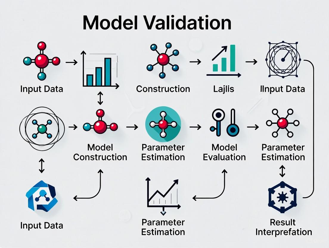
A Framework for Effective Model Validation
Executing a robust validation strategy requires a systematic, multi-faceted approach. The following workflow outlines the key stages, from data preparation to final analysis, which are expanded upon in the subsequent sections.
Model Validation Workflow
Data Validation and Conceptual Review
The foundation of any valid model is high-quality, relevant data and a sound conceptual framework.
Data Validation: Before a model can be validated, the data used for that validation must be trustworthy. This involves checking for and addressing missing values, outliers, and errors that could mislead the model [4]. Furthermore, the data must be a true representation of the underlying problem. In drug discovery, for instance, using cell-line data to validate a model predicting human in vivo efficacy requires careful consideration of the data's relevance and potential translational gaps [1]. It is also critical to assess data for bias, ensuring it has appropriate representation to avoid producing biased or inaccurate results [4].
Conceptual Review: This step involves a critical evaluation of the model's underlying logic and assumptions. Researchers must ask: Is the selected computational technique suitable for the biological or chemical problem at hand? Are the assumptions embedded in the model building—for example, about binding kinetics or cell behavior—justified and clearly understood? [4] Faulty assumptions can lead to a model that is conceptually elegant but practically useless.
Key Validation Techniques and Metrics
With a solid foundation in place, specific technical methods are employed to quantitatively and qualitatively assess the model's performance.
Comparison with Experimental Data: This is the "gold standard" for validation [2]. In practice, this means comparing the model's predictions against data obtained from controlled laboratory experiments. For example, a finite element analysis (FEA) prediction of strain in a material would be compared against measurements from physical strain gauges [2]. In computational drug design, a model predicting a compound's binding affinity must be validated against experimental data from sources like PubChem or the Cancer Genome Atlas, which provide empirical measurements on molecular structures and activities [1].
Benchmarking and Analytical Solutions: When direct experimental data is scarce or initial validation is needed, comparing model results against established analytical solutions or benchmark problems from scientific literature is a highly effective strategy [2] [3]. This provides a reality check against known results before venturing into novel predictions.
Data-Splitting Techniques: To avoid overfitting—where a model performs well on its training data but fails on new data—it is essential to test it on unseen data.
- Train/Test Split: The dataset is divided into a training set to develop the model and a separate testing set to assess its prediction accuracy on new observations [4]. Common split ratios are 70-30 or 80-20.
- Cross-Validation: A more robust technique, such as k-Fold Cross-Validation, involves dividing the data into 'k' subsets. The model is trained and evaluated 'k' times, each time using a different fold as the test set and the remaining folds for training. This provides a more comprehensive assessment of model performance [4].
Table: Key Performance Metrics for Model Validation
| Metric Category | Specific Metric | Definition and Application Context |
|---|---|---|
| Classification | Accuracy, Precision, Recall, F1-Score | Used for categorical outcomes (e.g., classifying a molecule as active/inactive) [4] |
| Regression | Mean Squared Error (MSE), R-squared | Quantifies the difference between predicted and actual continuous values (e.g., predicting binding affinity) [4] |
| Physical Sciences | Strain/Stress Correlation, Concentration Profile Match | Measures the agreement between simulated and experimentally measured physical quantities [2] |
Practical Application: Validation in Scientific Disciplines
The principles of model validation are universal, but their application varies significantly across scientific domains, each with its own unique challenges and best practices.
Validation in Drug Discovery and Development
Computational models in drug development face unique validation challenges due to the complexity of biological systems and the long timelines of clinical experiments.
- Leveraging Public Data: Given that clinical experiments on drug candidates can take years, a primary validation strategy is to compare a proposed drug candidate to the structure, properties, and efficacy of existing drugs using vast public databases like the Cancer Genome Atlas and those from the National Library of Medicine [1]. This provides a critical benchmark for early-stage validation.
- Multi-scale Validation: A model must be validated at multiple levels. A molecular dynamics simulation might be validated against crystallographic data for protein-ligand binding, while a systems pharmacology model would require validation against in vitro or in vivo efficacy and toxicity data.
- Synthesizability and Validity: In molecular design and generation studies, computational findings must be demonstrated to have practical usability. Experimental data confirming the synthesizability and biological validity of newly generated molecules is a powerful form of validation [1].
Validation in the Physical Sciences
In fields like chemistry and materials science, there is often a community expectation that computational work is paired with an experimental component [1].
- Chemistry: For studies in molecular design, experimental data that confirms the synthesizability and validity of newly generated molecules is crucial for verifying computational findings [1]. Without this, claims that a new catalyst or drug candidate outperforms existing ones can be difficult to substantiate.
- Materials Science: If a theoretical prediction points to a new class of materials with exotic properties, then experimental synthesis, materials characterization, and tests within real devices are typically required to support the prediction [1]. The growing availability of experimental data through initiatives like the High Throughput Experimental Materials Database presents exciting opportunities for more effective validation.
The Scientist's Toolkit: Essential Research Reagents & Materials
Table: Key Reagents and Tools for Experimental Validation
| Item / Solution | Primary Function in Validation |
|---|---|
| Strain Gauges | A reliable method for collecting physical deformation data to directly compare with FEA predictions of stress and strain [2] |
| PubChem / OSCAR Databases | Provide existing experimental data on molecular structures and properties for comparison with computational chemistry predictions [1] |
| Cancer Genome Atlas | A source of genomic, epigenomic, and clinical data used to validate bioinformatic models and computational findings in oncology [1] |
| Cell-based Assay Kits | Provide standardized biological readouts (e.g., viability, cytotoxicity) to validate models predicting biological activity in drug discovery |
| High-Throughput Experimental Materials Database | A source of empirical materials data used to validate predictions from computational materials science models [1] |
Model validation is not a one-time activity to be performed after a model is built; it is an integral, ongoing part of the computational research lifecycle. For researchers and drug development professionals, skipping rigorous validation carries significant risks, including false confidence in flawed designs, costly mistakes from decisions based on incorrect data, and a fundamental lack of credibility for their work, especially in regulated industries [2].
The ultimate goal of validation is to achieve model generalization—the ability of a model to make accurate predictions on new, unseen data [4]. This is the true test of a model's utility in a research or development setting. By moving beyond merely "solving the equations right" to rigorously determining that they are "solving the right equations," computational scientists can ensure their work is not just mathematically elegant, but physically meaningful and practically useful, thereby accelerating scientific discovery and innovation.
In computational science research, the integrity of a model determines the validity of its predictions. Models, whether mathematical, simulation-based, or physical, are representations of real-world processes used for studying, experimenting, or predicting real-world events [5]. However, as statistician George E.P. Box famously noted, "Essentially, all models are wrong, but some are useful" [5]. The utility of any scientific model is not inherent but must be rigorously demonstrated through systematic processes—verification and validation. These two distinct but complementary processes form the foundation of credible computational science, ensuring models are both technically correct and scientifically relevant.
The failure to distinguish between verification and validation represents a critical pitfall for many practitioners. Some use the terms interchangeably, while others perform one process while neglecting the other [5]. This leads to unrealistic predictions, misguided results, and ultimately, a loss of model integrity. In fields such as drug development, where computational models increasingly inform critical decisions, the ramifications of using unverified or invalidated models can be severe, potentially compromising research outcomes and patient safety. This guide examines the fundamental differences between verification and validation, provides detailed methodologies for their implementation, and frames their necessity within the broader context of scientific rigor in computational research.
Fundamental Concepts and Definitions
What is a Model?
A model is a simplified representation of a real-world process designed to study relationships between independent variables (inputs) and dependent variables (outcomes) [5]. Models serve as experimental platforms where researchers can observe system behavior without directly intervening in the actual process. In computational science, models typically fall into three categories:
- Mathematical models: Represent systems through equations and formulas (e.g., Little's Law in queuing theory)
- Simulation models: Implement mathematical representations in software to emulate system behavior over time
- Physical models: Scaled or analog representations of systems, common in engineering and architectural applications
Verification: Building the Model Right
Verification is the process of ensuring that a model correctly implements the intended relationships between input and output variables as conceived by the modeler [5]. It answers the fundamental question: "Was the model built correctly?"
Verification is an internal consistency check concerned with whether the computational model accurately solves the equations and implements the logic intended by its designers. It does not assess whether the model represents reality accurately, but rather whether it performs as its designers believe it should. For example, if a model is designed to return a rounded-up integer value of X1 divided by X2, verification confirms it returns 1 when X1=3 and X2=4, rather than 0.75 [5].
Validation: Building the Right Model
Validation is the process of determining whether a model accurately represents the real-world system it is intended to simulate [5]. It answers the fundamental question: "Was the correct model built?"
Validation ensures the model's outputs correspond to observed behaviors in the actual system through comparison with empirical data. It assesses the model's operational usefulness and predictive capability within its intended domain. As one comprehensive review of validation methods notes, validity in the social sciences "very generally refers to the question of whether measures actually measure what they are designed to measure," underpinning "the very essence of scientific progress" [6].
Table 1: Core Differences Between Verification and Validation
| Aspect | Verification | Validation |
|---|---|---|
| Primary Question | Was the model built correctly? | Was the correct model built? |
| Focus | Internal consistency and implementation | Correspondence to real-world behavior |
| Basis of Assessment | Model specifications and design | Empirical data from the actual system |
| Dependencies | Independent of real-world data | Heavily dependent on real-world data |
| Primary Methods | Code review, unit testing, convergence studies | Statistical comparison, hypothesis testing, expert judgment |
| Outcome | Error-free implementation that matches designer intent | Credible representation of the real system |
The Critical Distinction: Why Both Processes Are Essential
Verification and validation serve complementary but fundamentally different roles in model development. The relationship between these processes can be visualized as a sequential workflow where each stage addresses distinct aspects of model credibility:
Sequential Dependency and Iteration
Verification necessarily precedes validation in effective model development [5]. This sequence is logical—there is little value in comparing a model to real-world data if the model contains implementation errors that prevent it from executing as intended. However, the process is often iterative: validation may reveal issues that require returning to verification or even model redesign.
As highlighted in research on validation experiments, the design of validation activities should be directly relevant to the model's purpose—predicting a Quantity of Interest (QoI) at a prediction scenario [7]. This underscores the importance of aligning both verification and validation with the ultimate goals of the modeling effort.
Consequences of Confusion
The consequences of confusing verification and validation, or performing one without the other, are significant:
- Unverified but validated models may appear to match reality by compensating for implementation errors with incorrect parameter settings, but will fail when applied to new scenarios
- Verified but unvalidated models will precisely implement incorrect assumptions, providing false confidence in flawed representations
- Resource misallocation occurs when teams expend effort validating fundamentally flawed implementations or verifying models that represent the wrong system
Methodologies and Experimental Protocols
Verification Methodologies
Verification employs a suite of software and model engineering techniques to ensure correct implementation:
Code Review and Static Analysis
- Objective: Identify implementation errors through systematic examination
- Protocol: Structured walkthroughs, automated static analysis tools, peer review
- Metrics: Code coverage, complexity measures, standards compliance
Unit Testing and Algorithm Verification
- Objective: Verify individual components and algorithms in isolation
- Protocol: Develop tests for specific functions with known expected outcomes
- Example: For a rounding function, verify input-output pairs: (3/4)→1, (5/2)→3, etc. [5]
Solution Verification
- Objective: Ensure numerical solutions meet accuracy requirements
- Protocol: Convergence studies, grid independence tests, numerical error estimation
- Metrics: Residuals, convergence rates, error norms
Table 2: Verification Techniques and Their Applications
| Technique | Primary Application | Key Metrics | Limitations |
|---|---|---|---|
| Code Review | All model types | Compliance with standards, identified defects | Subject to human error, time-consuming |
| Unit Testing | Modular code structures | Test coverage, pass/fail rates | May not catch integration issues |
| Convergence Studies | Numerical models | Convergence rates, error estimates | Requires multiple model executions |
| Symbolic Verification | Mathematical models | Analytical equivalence | Limited to tractable mathematical representations |
Validation Methodologies
Validation methodologies compare model outputs with empirical data using rigorous statistical and expert-driven approaches:
Comparison with Experimental Data
- Objective: Quantify agreement between model predictions and observed system behavior
- Protocol:
- Collect high-quality experimental data under controlled conditions
- Run model with identical inputs and initial conditions
- Compare outputs using statistical measures
- Metrics: Mean error, confidence intervals, validation metrics
Predictive Validation
- Objective: Assess model capability to predict system behavior not used in model development
- Protocol:
- Reserve portion of experimental data for validation only
- Develop model using remaining data
- Compare predictions with validation dataset
- Metrics: Prediction error, confidence in predictions
Expert Assessment
- Objective: Leverage domain knowledge to assess model plausibility
- Protocol: Structured expert elicitation, Delphi methods, peer review
- Metrics: Qualitative assessment, plausibility ratings
As noted in a comprehensive review of topic modeling validation, there is a "notable absence of standardized validation practices" across computational social sciences [6]. This highlights the need for discipline-specific validation frameworks while maintaining scientific rigor.
Optimal Design of Validation Experiments
Advanced validation approaches emphasize designing validation experiments specifically tailored to the model's intended predictive purpose:
Influence Matrix Methodology
- Objective: Select validation scenarios most representative of prediction scenarios
- Protocol: Compute influence matrices characterizing response surfaces of model functionals, minimize distance between validation and prediction influence matrices [7]
- Application: Particularly valuable when prediction scenarios cannot be experimentally replicated
Sensitivity-Based Validation
- Objective: Ensure validation scenarios reflect sensitivities relevant to prediction
- Protocol: Use sensitivity indices (e.g., Sobol indices) to weight validation observations according to their relevance to QoI prediction [7]
- Application: Guides resource allocation to most influential validation activities
The relationship between model components, validation activities, and prediction goals can be visualized as an integrated system:
Case Studies and Applications
Case Study 1: Ice Cream Stand Queuing Model
A modeler builds a queuing model for an ice cream stand to predict customer waiting time (W) based on number of customers (X) in line [5].
Verification Process:
- Model implements equation W = 3X based on observed service rate of 3 minutes/customer
- Testing with inputs X=1,2,5,10,20 returns W=3,6,15,30,60 minutes respectively
- Verification confirms model correctly implements the linear relationship
Validation Process:
- Field observation of actual customer Jessica's waiting time across different queue lengths
- Real-system behavior diverges from model: customers leave when waiting exceeds tolerance
- Actual waiting times shorter than predicted linear relationship
- Model fails validation despite passing verification
Implication: A verified but invalid model produces quantitatively precise but practically useless predictions.
Case Study 2: Distribution Center Simulation
An LSS team develops a simulation model for a distribution center with four product-sorting machines [5].
Initial Findings:
- Model shows excessive queue at Machine B despite equal product distribution
- Model passed verification but produces counterintuitive results
Root Cause Analysis:
- Verification confirmed parameter entry matched design
- Detailed review discovered data entry error: 15 minutes instead of 1.5 minutes for Machine B processing time
- Correction enabled accurate system representation
Implication: Without validation, implementation errors can remain undetected despite verification.
Case Study 3: Pollutant Transport Model
A study on optimal validation design examines a pollutant transport model [7].
Challenge: Predicting contaminant concentration at sensitive location (QoI) where direct measurement is impossible
Solution:
- Designed validation experiments using influence matrices to match prediction scenario sensitivities
- Selected observation locations and conditions that best represented QoI scenario
- Quantified predictive uncertainty based on validation under representative conditions
Implication: Strategic validation design enables confidence in predictions even when QoI cannot be directly measured.
Table 3: Research Reagent Solutions for Model Verification and Validation
| Tool Category | Specific Solutions | Function | Application Context |
|---|---|---|---|
| Verification Tools | Unit testing frameworks (e.g., pytest, JUnit), Static analysis tools (e.g., SonarQube), Continuous integration systems | Automated error detection, Regression testing, Code quality assessment | Software implementation verification |
| Validation Data Sources | Experimental data repositories, Historical system data, Sensor networks, Expert elicitation protocols | Provide empirical basis for comparison, Ground truth establishment | Model validation across domains |
| Statistical Comparison Tools | Statistical software (e.g., R, Python SciPy), Bayesian calibration tools, Uncertainty quantification libraries | Quantitative comparison of model and data, Uncertainty propagation, Validation metrics calculation | Quantitative validation assessment |
| Sensitivity Analysis Tools | Sobol index calculators, Morris method implementations, Active subspace methods | Identify influential parameters, Guide validation resource allocation, Understand model behavior | Validation experiment design |
| Domain-Specific Benchmarks | Standard problems community, Reference implementations, Analytical solutions | Provide known solutions for comparison, Establish minimum capability requirements | Discipline-specific verification and validation |
Verification and validation represent complementary but fundamentally different processes essential to credible computational science. Verification ensures models are built correctly according to specifications, while validation ensures the correct models are built to represent reality. This distinction is not merely academic—it underpins the scientific utility of computational models across disciplines from engineering to drug development.
As computational models increase in complexity and application to critical decisions, the rigorous implementation of both verification and validation becomes increasingly essential. The methodologies and case studies presented provide a framework for researchers to implement these processes systematically, while the visualization of their relationships offers conceptual clarity. By embracing both verification and validation as distinct but essential practices, the computational science community can advance both the credibility and utility of computational modeling for scientific discovery and practical application.
The broader thesis of model validation in computational science research affirms that without rigorous validation, even perfectly verified models remain potentially misleading abstractions. As models continue to inform critical decisions in drug development, public policy, and engineering design, the commitment to both verification and validation represents not merely technical diligence but scientific and ethical responsibility.
Model validation provides the critical foundation for trust and reliability in computational science, particularly in the high-stakes field of drug development. It serves as a essential quality assurance process that evaluates how well a predictive model performs on new, unseen data, confirming that it achieves its intended purpose [4]. In Model-Informed Drug Development (MIDD), a "fit-for-purpose" approach to validation is paramount, ensuring that models are well-aligned with the specific Question of Interest (QOI) and Context of Use (COU) at each development stage [8]. Without rigorous validation, models are prone to validity shrinkage—a significant reduction in predictive performance when applied to new datasets—which can lead to costly late-stage failures and inaccurate regulatory decisions [9]. This technical guide examines the methodologies, metrics, and practical applications of model validation that underpin robust computational research in pharmaceutical sciences.
The Critical Role of Model Validation in Computational Science
Model validation is the systematic process of assessing a trained model's performance on new or unseen data, moving beyond mere mathematical correctness to evaluate real-world applicability [4]. In computational science research, this process transforms a theoretical model into a verified tool for scientific discovery and decision-making.
The core challenge addressed by validation is overfitting, where a model learns not only the underlying signal in the training data but also the random noise, resulting in poor generalization to new data [4]. The phenomenon of validity shrinkage describes the nearly inevitable reduction in predictive ability when a model derived from one dataset is applied to another [9]. This occurs because algorithms adjust model parameters to optimize performance metrics, fitting both the true signal and idiosyncratic noise from measurement error and random sampling variance [9].
The implications of unvalidated models in drug development are particularly severe. Without proper validation, researchers cannot justifiably rely on a model's predictions [4]. In critical domains, errors can have profound consequences, potentially leading to significant patient harm due to incorrect decisions made by models in real-world applications [4].
Table 1: Key Terminology in Model Validation
| Term | Definition |
|---|---|
| Validity Shrinkage | The reduction in predictive ability when a model moves from the data used for construction to a new, independent dataset [9]. |
| Stochastic Shrinkage | Validity shrinkage occurring due to variations from one finite sample to another [9]. |
| Generalizability Shrinkage | Validity shrinkage occurring when a model is applied to data from a different population than the one it was built in [9]. |
| Overfitting | When a model is overly adjusted to fit the training data and fails to predict new data accurately [4]. |
| Underfitting | When a model is too weak and cannot capture the true relationships in the data [4]. |
| Context of Use (COU) | A clearly defined description of how a model should be used and the specific purpose it serves [8]. |
Core Methodologies for Model Validation
Validation Techniques and Protocols
Multiple validation techniques have been developed to assess model performance across different data scenarios. The selection of an appropriate method depends on factors such as dataset size, data structure, and the specific modeling objectives.
Hold-out Methods represent the most fundamental approach to model validation. The Train-Test Split involves randomly dividing the dataset into two parts: one for training the model and a separate portion for testing its performance [10]. For smaller datasets (1,000-10,000 samples), an 80:20 ratio is typically recommended, while medium datasets (10,000-100,000 samples) may use a 70:30 ratio, and large datasets (over 100,000 samples) often employ a 90:10 ratio [10]. The Train-Validation-Test Split extends this approach by creating three distinct data partitions, with the validation set used for parameter tuning and the test set reserved for a single, final evaluation to provide an unbiased assessment of model performance [10].
Cross-Validation Techniques offer more robust evaluation, particularly for limited datasets. K-Fold Cross-Validation divides the data into k subsets (folds), training the model k times while using a different fold as the test set each time and averaging the results [4]. This provides a more extensive analysis than simple hold-out methods [4]. Leave-One-Out Cross-Validation (LOOCV) represents an extreme case of k-fold cross-validation where k equals the number of data points, offering a comprehensive assessment at significant computational expense [4]. Stratified K-Fold Cross-Validation maintains the same ratio of classes/categories in each fold as the overall dataset, which is particularly valuable when dealing with imbalanced data where one class has significantly fewer instances [4].
Advanced and Specialized Methods address specific validation challenges. Nested Cross-Validation combines an outer loop for model evaluation with an inner loop for hyperparameter tuning, assessing how well the model generalizes while simultaneously optimizing parameters [4]. Time-Series Cross-Validation respects temporal dependencies in data by splitting datasets in a way that maintains chronological order, ensuring models are evaluated on future observations rather than randomly partitioned data [4].
The following workflow diagram illustrates the relationship between these key validation methodologies:
Performance Metrics and Quantitative Assessment
Selecting appropriate performance metrics is fundamental to meaningful model validation. These metrics must align with the specific problem type—classification, regression, or time-to-event analysis—and the clinical context of use.
Table 2: Essential Validation Metrics for Different Model Types
| Model Type | Key Metrics | Interpretation | Application Examples |
|---|---|---|---|
| Classification | Sensitivity (Recall) | Proportion of true positives correctly identified [9] | Identifying liver fibrosis in hepatitis C patients [9] |
| Specificity | Proportion of true negatives correctly identified [9] | Identifying risk for undiagnosed diabetes [9] | |
| AUC (Area Under ROC Curve) | Overall measure of model's ability to distinguish classes [9] | Predicting obesity risk from genetic loci [9] | |
| Positive Predictive Value (PPV) | Proportion of positive predictions that are correct [9] | Diabetes remission after gastric bypass [9] | |
| Regression | R² (Coefficient of Determination) | Proportion of variance explained by the model [9] | Body composition prediction equations [9] |
| Adjusted R² | R² modified for number of predictors relative to sample size [9] | More reliable for multi-predictor models [9] | |
| Mean Squared Error (MSE) | Average squared difference between predicted and actual values [9] | Calibration models for insulin sensitivity [9] | |
| Shrunken R² | R² adjusted for expected validity shrinkage in new samples [9] | Provides conservative performance estimate [9] | |
| Survival/Time-to-Event | Concordance Index (c-index) | Measures agreement between predicted and observed event orders [9] | Similar to AUC but for time-to-event data [9] |
The Researcher's Toolkit: Essential Reagents for Model Validation
Implementing robust model validation requires both computational tools and methodological frameworks. The following table outlines key components of the validation toolkit:
Table 3: Essential Research Reagent Solutions for Model Validation
| Tool/Reagent | Function | Application Context |
|---|---|---|
| Stratified Sampling | Ensures representative distribution of classes in training/test splits | Prevents biased performance estimates with imbalanced data [4] |
| Bootstrap Methods | Estimates sampling distribution by drawing random sets with replacement | Quantifies uncertainty and expected validity shrinkage [9] |
| Hyperparameter Tuning | Optimizes model parameters not learned during training | Improves model performance via grid search or random search [4] |
| Statistical Tests (e.g., Wilcoxon Signed-Rank) | Compares performance between different models | Determines if performance differences are statistically significant [4] |
| Adjusted/Shrunken R² | Adjusts performance metrics for model complexity | Provides realistic expectation of performance in new data [9] |
Model Validation in the Drug Development Pipeline
Model validation takes on critical importance in the pharmaceutical industry, where the MIDD framework relies on quantitative models to accelerate hypothesis testing, assess drug candidates more efficiently, and reduce costly late-stage failures [8]. A "fit-for-purpose" approach ensures that validation strategies are closely aligned with the specific questions and contexts at each development stage [8].
The following diagram illustrates how validation activities integrate throughout the drug development lifecycle:
Validation Approaches Across Development Stages
Discovery Stage validation focuses on computational models like Quantitative Structure-Activity Relationship (QSAR) that predict biological activity based on chemical structure [8]. Validation at this stage typically involves leave-one-out cross-validation or external validation using separate chemical classes not included in model training.
Preclinical Research utilizes Physiologically Based Pharmacokinetic (PBPK) models and First-in-Human (FIH) dose algorithms [8]. Validation requires verifying that model predictions align with observed animal study results and can accurately extrapolate to human physiology.
Clinical Research employs Population Pharmacokinetics (PPK) and Exposure-Response (ER) models to explain variability in drug exposure and effects across individuals [8]. Validation uses k-fold cross-validation and bootstrap methods to estimate how well models will perform in broader patient populations.
Regulatory Review and Post-Market Monitoring require continuous validation as models are applied to larger, more diverse populations [8]. This includes monitoring model performance against real-world evidence and updating models when performance degrades.
Model validation represents a fundamental discipline in computational science that bridges theoretical modeling and real-world application. In drug development, where decisions have profound implications for patient safety and therapeutic success, rigorous validation is not merely optional but ethically and scientifically essential. By implementing the methodologies, metrics, and frameworks outlined in this technical guide—from cross-validation techniques to performance metrics and fit-for-purpose approaches—researchers can build trustworthy models that reliably inform critical development decisions. As artificial intelligence and machine learning assume increasingly prominent roles in pharmaceutical research [8], the principles of model validation will remain the foundation upon which reliable, ethical, and effective drug development depends.
In computational science research, the integrity of model-based conclusions is paramount. A robust validation framework is the cornerstone of credible research, ensuring that computational models are not only mathematically sound but also scientifically meaningful and reliable in their predictions. This framework provides a structured defense against model risk—the potential for adverse consequences from decisions based on incorrect or misused model outputs [11]. Within regulated fields like drug development, a "fit-for-purpose" approach is increasingly emphasized, requiring that the validation process be closely aligned with the model's intended context of use and the key questions of interest it aims to address [8]. This guide details the three core components—Data, Conceptual, and Testing elements—that form the foundation of a rigorous validation protocol, providing researchers and drug development professionals with the methodologies to build trust in their computational tools.
Core Component 1: Data Validation
Data validation ensures the quality and relevance of the information used to build and test models, adhering to the principle that a model's output is only as reliable as its input data [12]. This component is critical for preventing the perpetuation of data errors and biases into the model's predictions.
Key Elements and Quantitative Checks
The following table summarizes the core elements of data validation and their associated quantitative checks:
| Data Validation Element | Description | Key Quantitative Checks & Methods |
|---|---|---|
| Data Quality | Ensuring data is accurate, complete, and free from errors that could skew model learning [4]. | - Handle missing values (e.g., imputation or removal)- Detect and manage outliers to prevent skewed predictions [13]- Perform data quality checks on sources, especially third-party data [12] |
| Data Relevance | Verifying the data is a true representation of the underlying problem the model is designed to solve [4]. | - Confirm data represents the scenarios the model will encounter [13]- Assess whether data sources are appropriate for the model's intended purpose [12] |
| Bias and Representation | Checking for appropriate representation to avoid reproducing biased or inaccurate results [4]. | - Analyze data demographics- Use unbiased sampling methods [4]- Scrutinize data for accuracy, completeness, and bias; log treatment of missing values and proxies [12] |
Experimental Protocols for Data Validation
- Protocol for Handling Missing Data: Identify missing values through summary statistics and data visualization. Decide whether to remove records with missing values or to fill them in using techniques such as mean/median imputation for numerical data or mode imputation for categorical data. The choice must be documented, noting the potential impact on the model [13] [12].
- Protocol for Ensuring Representativeness: Compare the distributions of key variables in your dataset against the known distributions in the target population or against a reference dataset. Use statistical tests (e.g., Chi-square tests for categorical data, KS-test for continuous data) to identify significant deviations. For biased datasets, employ techniques like stratified sampling to ensure the training data is representative [4].
- Protocol for Bias Mitigation: Analyze model features to determine if any are proxies for protected class membership (e.g., race, gender). This involves evaluating the correlation between features and protected attributes. Techniques such as reweighting or adversarial debiasing can then be applied to mitigate identified biases [12].
Core Component 2: Conceptual Soundness
Conceptual soundness evaluation assesses the quality of the model's design and theoretical foundation. It ensures that the model's logic, assumptions, and construction are well-informed, carefully considered, and consistent with established scientific principles and the intended business or research objective [11] [12].
Foundational Elements
A conceptually sound model is built upon a logical design that is appropriate for the problem at hand. This involves a critical review of the chosen algorithms and techniques to ensure they are suitable [4]. Furthermore, the model's variables must be relevant and informative to the model's purpose; extraneous variables can lead to poor predictions, while omitting key variables can render the model ineffective [4]. A core aspect of this review is the explicit documentation and understanding of all assumptions embedded in the model's construction. Unchecked invalid assumptions can directly lead to inaccurate forecasts and model failure [4] [14].
Methodologies for Evaluation
- Review of Documentation and Empirical Evidence: Scrutinize the model's documentation to ensure it is sufficiently detailed to allow parties unfamiliar with the model to understand its operation, limitations, and key assumptions [11]. The documentation should provide empirical evidence and reference published research supporting the methods and variables selected.
- Expert-Logical Soundness Analysis: Engage subject matter experts to critically evaluate the model's logic and its alignment with domain knowledge [13]. This involves questioning whether the model's design and the relationships it posits are consistent with sound industry practice and scientific understanding [11].
- Benchmarking Against Established Models: Compare the model's design, theoretical foundation, and outputs to alternative models or established industry approaches. This helps verify that the model's methodology is sound and its results are reasonable within the context of existing knowledge [11].
Core Component 3: Testing and Ongoing Monitoring
Testing and ongoing monitoring provide empirical evidence of a model's performance and ensure its reliability throughout its lifecycle. This component moves from theoretical validation to practical verification under various conditions and over time.
Performance Metrics and Testing Techniques
Selecting the right performance metrics is essential to determine how well a model will perform on new data [13]. The choice of metrics depends on the model's purpose (e.g., classification, regression).
| Model Task | Key Performance Metrics | Description and Use Case |
|---|---|---|
| Classification | Accuracy, Precision, Recall, F1 Score, ROC-AUC | Measures the model's ability to correctly classify and distinguish between classes. F1 score combines precision and recall, while ROC-AUC evaluates performance across thresholds [13] [4]. |
| General | Outcomes Analysis (Back-testing) | Comparing model outputs to corresponding actual outcomes during a time period not used in model development [11]. |
| Stability & Robustness | Sensitivity Analysis, Stress Testing | Testing how model outputs change when inputs vary or are pushed to extreme values to assess stability and identify limitations [12]. |
Key Testing Techniques:
- Train/Test Split & Cross-Validation: The dataset is divided into a training set to develop the model and a testing set to assess its prediction accuracy on new observations [4]. For a more robust evaluation, K-Fold Cross-Validation is preferred, where the data is divided into k subsets and the model is trained and evaluated k times, each time using a different fold as the test set [13] [4].
- Ongoing Monitoring: Model monitoring is not a one-time activity. It involves continuously tracking the model's performance and the data it receives to detect issues like model drift [13] [12]. Effective monitoring includes:
- Population Stability: Tracking whether the input data remains consistent with the data used for development.
- Performance Drift: Monitoring for decay in the model's predictive accuracy over time.
- Data Quality Maintenance: Ensuring ongoing data meets the same quality standards as the training data [12].
Experimental Protocols for Testing
- Protocol for K-Fold Cross-Validation:
- Randomly shuffle the dataset and partition it into k roughly equal-sized folds (commonly k=5 or k=10).
- For each unique fold: a) Use the fold as the validation data (test set). b) Use the remaining k-1 folds as the training data. c) Fit a model on the training set and evaluate it on the test set. d) Retain the evaluation score.
- Calculate the average of the k evaluation scores to produce a single robust estimation of model performance. This method provides a more comprehensive analysis than a single train/test split [13] [4].
- Protocol for Outcomes Analysis (Back-testing):
- Reserve a portion of the dataset from a time period not used in the model's development.
- At a frequency that matches the model's forecast horizon, compare the model's predictions against the actual, realized outcomes.
- Use statistical tests to determine if the differences between predictions and outcomes are significant and fall outside the organization's predetermined thresholds of acceptability [11].
- Protocol for Monitoring Data Drift:
- Establish a baseline distribution for key input variables from the model's training data.
- At a regular cadence (e.g., daily, weekly), compute the distribution of the same variables from the live, incoming data.
- Use a statistical distance metric (e.g., Population Stability Index (PSI), Kullback-Leibler divergence) to quantify the difference between the live data distribution and the baseline.
- Trigger an alert and initiate a model review process if the metric exceeds a predefined threshold [12].
A successful validation process relies on a combination of statistical tools, software libraries, and governance frameworks. The table below details key resources essential for implementing a robust validation framework.
| Tool Category | Specific Examples | Function in Validation |
|---|---|---|
| Statistical & ML Libraries | Scikit-learn, TensorFlow, PyTorch [13] | Provide built-in functions for cross-validation, performance metrics (accuracy, precision, recall, F1-score), and model evaluation APIs. |
| Specialized Validation Platforms | Galileo [13] | Offer end-to-end solutions with advanced analytics, visualization, automated insights, and continuous monitoring for model drift detection. |
| Governance Frameworks | SR 11-7 Guidance on Model Risk Management [11] | Provides a regulatory-backed framework for model risk management, defining standards for development, validation, and governance. |
| Validation Checklists | FairPlay's Six-Step Model Validation Checklist [12] | Offers a practical, question-based framework for validating conceptual soundness, data quality, process, outcomes, and governance. |
The integration of rigorous data validation, conceptual soundness evaluation, and comprehensive testing forms an interdependent triad essential for any robust model validation framework in computational science. By adhering to this structured approach, researchers and drug development professionals can significantly mitigate model risk, enhance the credibility of their findings, and ensure their models are truly fit-for-purpose. As models grow in complexity and are applied in increasingly critical domains, a disciplined and documented validation process, supported by appropriate tools and checklists, transitions from a best practice to a non-negotiable standard of scientific rigor.
Model validation stands as a critical gatekeeper in computational science, ensuring that predictions translate reliably into real-world applications. In healthcare and biomedical research, where models inform diagnoses, treatment decisions, and therapeutic development, the stakes of inadequate validation are monumental. This whitepaper examines the severe consequences of validation failures, ranging from diagnostic inaccuracies and compromised patient safety to the erosion of trust in data-driven technologies. By synthesizing current research, we present a framework of rigorous validation methodologies and best practices designed to fortify computational models against failure, thereby safeguarding public health and accelerating the responsible deployment of artificial intelligence in medicine.
The integration of computational models and artificial intelligence (AI) into healthcare represents a paradigm shift in medical research and clinical practice. These technologies, built upon Medical Laboratory Data (MLD) and other complex datasets, hold the potential to revolutionize disease screening, diagnosis, and personalized medicine [15]. However, this potential is critically contingent on a foundational principle often overlooked in the rush to innovation: rigorous and comprehensive model validation. Validation is the multi-faceted process of evaluating a computational model to ensure its accuracy, reliability, and robustness for its intended purpose.
Within the context of computational science research, validation moves beyond a mere technicality; it is an ethical imperative. In fields such as drug development and clinical diagnostics, models guide decisions that directly impact human lives. A model that predicts patient response to a therapy, identifies malignant tissues in a radiological scan, or forecasts the spread of an infectious disease must be not only sophisticated but also demonstrably trustworthy. The consequences of inadequate validation are not merely statistical errors but can manifest as misdiagnoses, ineffective treatments, and significant patient harm. As noted in studies of model risk management, failures often stem from two broad sources: execution risk, where a model fails to perform its intended function, and conceptual errors, where incorrect assumptions or techniques are used in model development [16] [17]. This paper explores these high-stakes consequences and outlines the rigorous experimental protocols and validation frameworks necessary to mitigate them.
Consequences of Inadequate Model Validation
The failure to adequately validate computational models in healthcare can lead to a cascade of negative outcomes, which can be categorized into direct patient impacts, systemic research inefficiencies, and broader ethical and trust-related repercussions.
Diagnostic Inaccuracies and Patient Harm
The most immediate and severe consequence of model failure is the potential for direct harm to patients. Inaccurate models can lead to both false positives and false negatives, each with serious implications.
- Misdiagnosis and Delayed Treatment: AI models that fail to accurately identify diseases from medical laboratory data can lead to fatal delays in treatment. For instance, a model for early sepsis detection developed at the First Affiliated Hospital of Zhengzhou University demonstrated the high sensitivity (87%) and specificity (89%) required for reliable clinical use. An inadequately validated model with lower performance metrics would miss critical cases, delaying life-saving interventions [15].
- Inadequate Personalization of Therapy: Personalized medicine relies on models to tailor treatments based on individual patient data. A flawed model can lead to the selection of suboptimal or harmful therapeutic regimens. Research into models that analyze biomarkers like circulating tumor DNA has shown great promise in predicting cancer risk and monitoring progression. A validation failure in such a context could direct a patient toward an ineffective therapy while their disease continues to advance [15].
Compromised Data Quality and Research Integrity
The foundation of any reliable computational model is high-quality data. Inadequate validation protocols often fail to identify underlying data issues, corrupting the entire research process.
Table 1: Key Data Quality Dimensions and Consequences of Their Failure
| Data Quality Dimension | Description | Consequence of Inadequate Validation |
|---|---|---|
| Accuracy | The extent to which data are correct, reliable, and free from error [18]. | Leads to model predictions that are fundamentally misaligned with biological reality, causing misdiagnosis and treatment errors. |
| Completeness | The degree to which all required data is present [18]. | Introduces biases and reduces the statistical power of models, leading to unreliable and non-generalizable findings. |
| Reusability | The suitability of data for secondary use in different contexts, supported by metadata and documentation [18]. | Prevents the reproduction and independent verification of research findings, stalling scientific progress. |
Machine learning-based strategies have demonstrated the ability to significantly improve data quality, with one study achieving a rise in data completeness from 90.57% to nearly 100% through techniques like K-nearest neighbors (KNN) imputation [18]. Without validation processes that rigorously check for these dimensions, models are built on a fragile foundation.
Erosion of Trust and Hindered Innovation
Beyond immediate technical failures, inadequate validation has a corrosive effect on the broader ecosystem of computational biomedicine.
- Stifled Clinical Adoption: Clinicians are justifiably hesitant to adopt tools that lack transparent and proven validation records. The gap between AI model development and its deployment in clinical settings is largely attributable to a lack of a unified framework for applying AI to clinical decision-making processes [15].
- Reproducibility Crises: The inability to replicate published findings is a significant problem in computational science. As seen in other fields like Computational Fluid Dynamics (CFD), inconsistencies in documenting geometric fidelity, meshing strategy, and solver configuration can render published models useless for replication or validation, severely impeding scientific progress [19].
- Ethical and Regulatory Breaches: The use of poorly validated models can lead to violations of data privacy regulations (like GDPR and HIPAA) and ethical guidelines. Ensuring that models are fair, unbiased, and secure is an integral part of the validation process, and its failure can have legal and reputational consequences [15].
A Framework for Robust Validation: Methodologies and Protocols
To mitigate the severe risks outlined above, the biomedical research community must adopt a systematic and multi-layered approach to model validation. The following protocols provide a roadmap for ensuring model reliability.
Model Risk Management (MRM) and the Three Lines of Defense
A robust Model Risk Management (MRM) function, staffed by independent experts, is essential for governing a model's entire lifecycle. Best practices from financial risk management, which are highly applicable to healthcare, include [16] [17]:
- Model Tiering: Categorizing models based on their risk to the organization. High-tier models (e.g., those used for patient diagnosis or drug safety prediction) undergo the most rigorous validation, including comprehensive back-testing and frequent full-scope validations every two to three years.
- Continuous Monitoring: MRM should not be a point-in-time exercise. Model performance must be continuously monitored through reports produced by model owners at intervals matching the frequency of the model's use [16].
- Three Lines of Defense:
- First Line: Model developers and owners who own the risk and are responsible for initial quality control.
- Second Line: The independent MRM function that reviews, challenges, and validates models.
- Third Line: Internal audit functions that provide assurance to senior management on the effectiveness of the MRM framework [16].
Technical Validation Protocols and Workflows
The technical core of validation involves a set of experimental and computational protocols designed to stress-test the model.
Table 2: Experimental Protocols for Model Validation in Healthcare
| Protocol Category | Methodology | Key Performance Indicators (KPIs) |
|---|---|---|
| Data Quality Assessment | - Missing Value Imputation: Apply K-nearest neighbors (KNN) imputation [18].- Anomaly Detection: Use ensemble techniques like Isolation Forest and Local Outlier Factor (LOF) [18].- Dimensionality Reduction: Perform Principal Component Analysis (PCA) to identify key predictors. | - Completeness rate (%) pre- and post-imputation.- Number and type of anomalies detected and corrected.- Variance explained by principal components. |
| Performance Validation | - Train-Test Split: Split data into training and hold-out test sets.- Cross-Validation: Use k-fold cross-validation to assess stability.- Comparison to Benchmarks: Compare model performance against established clinical standards or existing methods. | - Accuracy, Sensitivity, Specificity.- Area Under the Curve (AUC) of the ROC curve.- Statistical significance of performance improvements. |
| Clinical Validation | - External Validation: Test the model on a completely independent dataset, ideally from a different institution [15].- Prospective Trials: Validate the model in a real-world clinical setting as part of a structured trial. | - Sensitivity/Specificity on external validation set.- Impact on clinical workflow and patient outcomes. |
The following workflow diagram synthesizes these protocols into a coherent validation pipeline for a healthcare AI model.
The Scientist's Toolkit: Essential Research Reagent Solutions
A robust validation pipeline relies on a suite of computational and data management "reagents." The following table details key components.
Table 3: Key Research Reagent Solutions for Model Validation
| Tool Category | Specific Examples | Function in Validation |
|---|---|---|
| Data Imputation & Cleaning | K-Nearest Neighbors (KNN) Imputation [18] | Addresses missing data to ensure completeness and reduce bias. |
| Anomaly Detection | Isolation Forest, Local Outlier Factor (LOF) [18] | Identifies and corrects outliers and erroneous data points that can skew model performance. |
| Dimensionality Reduction | Principal Component Analysis (PCA) [18] | Simplifies complex data, identifies key predictive variables, and helps in visualizing data patterns for quality assessment. |
| Predictive Modeling | Random Forest, LightGBM [18] | Provides robust, benchmarked algorithms for constructing predictive models whose performance can be rigorously validated. |
| Model Risk Management (MRM) | MRM Framework [16] [17] | Provides the organizational structure and governance for independent model review, tiering, and continuous monitoring. |
| Data Standards | FAIR Principles, HL7, HIPAA [15] | Ensures data is Findable, Accessible, Interoperable, and Reusable, and that its handling complies with privacy and security regulations. |
The integration of computational models into healthcare is inevitable and holds immense promise. However, this promise cannot be realized without an unwavering commitment to rigorous model validation. The consequences of cutting corners are unacceptably high, directly impacting patient safety, research integrity, and the credibility of data science as a discipline. By adopting a structured framework that combines independent model risk management, transparent technical protocols, and a commitment to continuous monitoring, the biomedical research community can build trustworthy and impactful AI systems. The path forward requires a cultural shift where validation is not seen as a final hurdle but as an integral, ongoing component of the computational science research lifecycle, ensuring that innovation always aligns with the principle of "first, do no harm."
Methodologies in Action: A Practical Guide to Validation Techniques for Computational Models
In computational science research, the validity of predictive models determines the reliability of scientific findings and the success of their practical applications. This technical guide examines the foundational validation methodologies of in-sample and out-of-sample testing, providing a comprehensive framework for researchers to evaluate model performance and generalizability. Through detailed protocols, quantitative comparisons, and practical implementations focused on drug development applications, we establish rigorous standards for model validation that ensure computational findings translate effectively into real-world solutions, thereby enhancing research reproducibility and application success.
Model validation represents a critical phase in the computational research pipeline, serving as the definitive process for evaluating a model's performance and confirming it achieves its intended purpose [4]. In computational disciplines, particularly in high-stakes fields like drug development, validation provides the essential link between theoretical models and their reliable application to real-world problems. The core objective is to assess how well a trained model performs on new or unseen data, moving beyond mere data fitting to genuine pattern recognition [20].
Without robust validation, researchers risk building models that appear effective but fail catastrophically when deployed. This is especially crucial in domains like healthcare and drug discovery, where model errors can have severe consequences, leading to significant fatalities due to incorrect decisions [4]. The validation process helps identify and mitigate potential biases, prevents overfitting and underfitting, and ultimately increases confidence in model predictions by providing transparency and explainability [4].
Two foundational paradigms dominate validation methodology: in-sample and out-of-sample approaches. Understanding their philosophical and practical distinctions forms the cornerstone of reliable computational research and enables scientists to make informed decisions about model deployment in critical applications.
Defining the Paradigms: Core Concepts and Terminology
In-Sample Validation
In-sample validation assesses a model's accuracy using the same dataset it was trained on [21]. This approach involves training a model on a dataset and then using that same dataset to generate predictions and calculate performance metrics [22]. For example, if you fit a linear regression model to predict monthly sales using data from 2010 to 2020, in-sample forecasts would predict sales for those same years [21]. Metrics like R-squared or Mean Squared Error (MSE) calculated through in-sample validation reflect how well the model fits the training data but risk overfitting—where a model memorizes noise or irrelevant patterns in the training data [21]. A high in-sample accuracy doesn't guarantee the model will perform well on new data [21].
Out-of-Sample Validation
Out-of-sample validation evaluates a model's performance on data it hasn't encountered during training [21]. This is typically accomplished by splitting the dataset into a training period (e.g., 2010-2018) and a test period (e.g., 2019-2020) before model development begins [21]. For time series data, the split must respect temporal order to avoid data leakage [21]. This method provides a more realistic estimation of how the model will perform in real-world scenarios on unseen data [22], helping identify overfitting and ensuring the model captures generalizable patterns rather than memorizing training artifacts [21].
Table 1: Fundamental Characteristics of Validation Approaches
| Characteristic | In-Sample Validation | Out-of-Sample Validation |
|---|---|---|
| Data Usage | Uses same data for training and testing [21] | Tests on unseen data not used during training [21] |
| Primary Function | Assess model fit to training data [22] | Evaluate model generalizability [23] |
| Overfitting Risk | High [21] | Lower [21] |
| Real-world Performance Estimate | Optimistic and potentially misleading [21] [24] | More realistic [21] [24] |
| Computational Demand | Generally efficient [22] | Can be intensive with cross-validation [22] |
Comparative Analysis: Advantages, Disadvantages, and Performance Metrics
Advantages and Disadvantages
The selection between in-sample and out-of-sample validation strategies involves balancing competing advantages and limitations based on research objectives, data characteristics, and application requirements.
In-sample validation offers computational efficiency, making it particularly valuable during initial model development phases when rapid iteration is necessary [22]. It provides immediate feedback on how well the model learns underlying patterns in the training data, helping researchers identify whether their model architecture can capture the complexity present in the dataset [22]. This approach facilitates direct model evaluation based on the same data used for training, offering insights into the model's learning capacity [22].
However, in-sample validation is profoundly prone to overfitting, where a model achieves high accuracy on training data but fails to generalize [21] [22]. This limitation is particularly problematic with complex models that can inadvertently memorize noise and outliers present in the training set rather than learning generalizable patterns [21]. Consequently, in-sample performance metrics often provide an overly optimistic and potentially misleading estimation of real-world performance [21] [24].
Out-of-sample validation addresses these limitations by providing a more accurate estimation of model performance on unseen data, effectively validating the model's effectiveness in real-world scenarios [22]. This approach represents the gold standard for detecting overfitting and verifying that the model has learned transferable patterns rather than training set specifics [21]. By testing on completely separate data, out-of-sample validation builds confidence in model deployments, particularly in critical applications like medical diagnosis or drug discovery [25] [4].
The primary disadvantages of out-of-sample validation include the requirement for a separate dataset for testing and potentially increased computational demands, especially when implementing multiple iterations or cross-validation techniques [22]. Additionally, proper out-of-sample validation requires careful experimental design, such as maintaining temporal sequences in time-series data, which adds complexity to the validation pipeline [21].
Quantitative Performance Comparison
Empirical studies across multiple domains consistently demonstrate the performance gap between in-sample and out-of-sample evaluations. In financial strategy development, quantitative analysis of 355 trading strategies revealed significant degradation in risk-adjusted returns when moving from in-sample to out-of-sample testing [26].
Table 2: Quantitative Performance Comparison of 355 Trading Strategies
| Performance Measure | In-Sample Results | Out-of-Sample Results | Absolute Change | Percentage Change |
|---|---|---|---|---|
| Average Sharpe Ratio | 1.574 | 1.049 | -0.525 | -33.37% |
| Median Sharpe Ratio | 1.180 | 0.662 | -0.518 | -43.90% |
This observed performance degradation aligns with findings across computational domains, where models typically exhibit superior performance on the data they were trained on compared to unseen data [26]. The magnitude of this gap serves as an important indicator of potential overfitting and model robustness, with smaller gaps generally indicating more generalizable models [26].
Methodological Implementation: Protocols and Workflows
Experimental Protocols for Out-of-Sample Validation
Implementing robust out-of-sample validation requires methodical experimental design. The following protocols ensure scientifically sound validation across different data environments:
Standard Holdout Protocol
- Data Partitioning: Split dataset into training and testing subsets, typically using 70-30 or 80-20 ratios depending on dataset size [4]. For smaller datasets (<10,000 samples), use 70-30 ratio; for medium datasets (10,000-100,000 samples), use 80-20 ratio; for large datasets (>100,000 samples), use 90-10 ratio [20].
- Temporal Preservation: For time-series data, maintain chronological order where training data precedes test data temporally to prevent data leakage [21].
- Single Evaluation: Evaluate the final model on the test set only once to prevent indirect optimization on the test set [20].
K-Fold Cross-Validation Protocol
- Dataset Division: Partition data into k subsets (folds) of approximately equal size [4].
- Iterative Training: Train the model k times, each time using k-1 folds for training and the remaining fold for validation [4].
- Performance Aggregation: Calculate final performance metrics as the average across all k iterations [4].
- Stratification: For classification problems, maintain class distribution ratios in each fold through stratified cross-validation [4].
Temporal Cross-Validation Protocol for Time-Series Data
- Rolling Window: Use expanding or sliding time windows for training with subsequent periods for testing [21].
- Fixed Horizon: Maintain consistent forecast horizons across validation cycles [21].
- Multiple Test Periods: Validate across different temporal regimes to assess model consistency [21].
Workflow Visualization
Applications in Computational Drug Discovery and Development
The distinction between in-sample and out-of-sample validation carries particular significance in computational drug repurposing, where accurate prediction models can significantly accelerate therapeutic development while reducing costs [25]. The rigorous drug repurposing pipeline involves making connections between existing drugs and new disease indications based on features collected through biological experiments or clinical observations [25].
In this domain, computational validation often begins with in-sample approaches to identify potential drug-disease connections, followed by essential out-of-sample validation using independent information sources not utilized during the prediction phase [25]. These validation sources may include previous experimental/clinical studies, protein interaction data, gene expression data, or other independent resources that provide supporting evidence for repurposing hypotheses [25]. This rigorous validation process helps reduce false positives and builds confidence in repurposed drug candidates before committing to expensive clinical trials [25].
Validation Strategies in Computational Drug Repurposing
Research by Brown et al. identified several validation strategies specifically employed in computational drug repurposing, which can be categorized as computational and non-computational approaches [25]:
Computational Validation Methods
- Retrospective Clinical Analysis: Utilizing EHR or insurance claims data to examine off-label drug usage or searching existing clinical trials databases for drug-disease connections [25].
- Literature Support: Manual literature searches or text mining of biomedical literature to find relevant articles containing connections between existing drugs and new therapeutic uses [25].
- Public Database Search: Leveraging specialized databases containing drug-target interactions, side effect profiles, or genomic associations [25].
- Benchmark Dataset Testing: Evaluating model performance against established gold-standard datasets within the field [25].
Non-Computational Validation Methods
- In Vitro Experiments: Laboratory testing of predicted drug-disease relationships in controlled cellular environments [25].
- In Vivo Studies: Animal model testing to validate therapeutic efficacy in whole organisms [25].
- Clinical Trials: Prospective evaluation of repurposing hypotheses through phased clinical trials [25].
- Expert Review: Domain expert evaluation of predictions based on pharmacological and clinical knowledge [25].
The Scientist's Toolkit: Essential Research Reagents and Materials
Table 3: Key Research Reagent Solutions for Validation Experiments
| Reagent/Material | Function in Validation | Application Context |
|---|---|---|
| Binding Affinity Assays (e.g., ELISA) | Quantify molecular interactions between drug compounds and targets [27] | Initial hypothesis testing for drug repurposing predictions |
| Enzyme Activity Assays | Measure functional biochemical responses to drug treatments [27] | Mechanistic validation of predicted drug effects |
| Cell Viability Assays | Monitor cellular health and metabolic responses to compound exposure [27] | Toxicity screening and therapeutic efficacy assessment |
| Microfluidic Devices | Enable controlled environment drug testing on cells [27] | Mimic physiological conditions for more realistic validation |
| Biosensors | Detect specific analytes with high sensitivity and specificity [27] | Fine-tune assay conditions and monitor biological parameters |
| Automated Liquid Handling Systems | Increase assay throughput and reproducibility [27] | Standardize validation protocols across multiple experiments |
In computational science research, particularly in high-stakes fields like drug development, the distinction between in-sample and out-of-sample validation represents more than a technical formality—it constitutes a fundamental principle of rigorous scientific methodology. While in-sample validation provides initial insights into model behavior and training efficiency, out-of-sample testing remains the unequivocal standard for establishing genuine model generalizability and real-world applicability [21] [4].
The consistent performance degradation observed when moving from in-sample to out-of-sample evaluation across multiple domains [26] underscores the critical importance of this distinction and highlights the risks of relying solely on training data performance metrics. For computational researchers and drug development professionals, implementing robust out-of-sample validation protocols is not merely best practice but an ethical imperative when model predictions may influence therapeutic development decisions [25].
As computational methodologies continue to evolve, embracing increasingly complex models with greater capacity for pattern recognition—and consequently, greater overfitting risks—the principles of rigorous validation outlined in this guide will only grow in importance. By adhering to these foundational approaches, researchers can ensure their computational findings translate effectively into tangible scientific advances and therapeutic breakthroughs.
In computational science research, particularly in high-stakes fields like drug development, the ability to generalize reliably to new, unseen data is the cornerstone of a valid predictive model. Model validation is not merely a final step but a fundamental principle that guards against overoptimism and ensures that scientific findings are robust and reproducible. This whitepaper details three core validation methodologies—Train-Test Split, K-Fold, and Leave-One-Out Cross-Validation—providing researchers and scientists with a structured comparison, detailed experimental protocols, and essential tools to integrate rigorous validation into their computational research pipelines.
The primary goal of supervised machine learning is to develop models that perform well on new, unseen data, a property known as generalization. In computational research, the development of a predictive model using a finite dataset is susceptible to overfitting, where a model learns patterns specific to the training data—including statistical noise—and fails to perform well on new data [28]. This creates a dangerous gap between expected and actual model performance, which can undermine scientific conclusions and the efficacy of a newly developed drug.
Model validation is the process that mitigates this risk by providing a realistic estimate of a model's generalization performance [4]. It is a critical step that moves beyond simple metrics on the data used for training. For healthcare and drug development professionals, rigorous validation is not just a technicality; it is an ethical imperative. Errors in predictive models can have severe consequences, leading to incorrect decisions in real-world applications [4]. This guide focuses on three foundational validation techniques that form the essential toolkit for any computational scientist.
Core Methodologies and Visual Workflows
This section outlines the core principles and workflows of the three key validation methods.
Train-Test Split (Holdout Method)
The Train-Test Split is the most straightforward validation approach. It involves randomly partitioning the entire dataset into two independent subsets: a training set used to train the model and a holdout test set used only once to evaluate the final model's performance [29] [4]. This one-time split ensures the model is evaluated on data it has never encountered during training.
K-Fold Cross-Validation
K-Fold Cross-Validation provides a more robust performance estimate by repeatedly performing train-test splits. The dataset is first divided into k equal-sized subsets (folds). The model is then trained and evaluated k times. In each iteration, a different fold is used as the test set, and the remaining k-1 folds are combined to form the training set. The final performance is the average of the scores from the k iterations [29] [30]. This method makes efficient use of all data points for both training and testing.
Leave-One-Out Cross-Validation (LOOCV)
Leave-One-Out Cross-Validation is an extreme case of k-fold cross-validation where the number of folds k is set equal to the number of instances n in the dataset [29]. This means the model is trained n times, each time using n-1 samples for training and the single remaining sample as the test set. The final performance is the average of all n evaluations.
Structured Comparison of Validation Techniques
The choice of validation strategy involves trade-offs between computational cost, the bias-variance of the estimate, and the characteristics of the available data. The following tables provide a structured comparison to guide this decision.
Table 1: Comparative Analysis of Core Validation Methods
| Feature | Train-Test Split | K-Fold Cross-Validation | Leave-One-Out (LOOCV) |
|---|---|---|---|
| Number of Splits | One time | k times (typically 5 or 10) [28] | n times (n = dataset size) [29] |
| Training Data Usage | Fixed percentage (e.g., 70-80%) | (k-1)/k of the data in each round [29] | (n-1) samples in each round [29] |
| Computational Cost | Low | High (model trained k times) [30] | Very High (model trained n times) [4] |
| Variance of Estimate | High (depends on a single split) [30] | Moderate | High (especially with outliers) [30] |
| Bias of Estimate | Higher (if dataset is small) [30] | Lower | Low (uses maximum data for training) [29] |
| Best Use Case | Very large datasets [28] or quick prototyping | Small to medium-sized datasets [29]; standard for model tuning | Very small datasets where maximizing training data is critical [29] |
Table 2: Key Evaluation Metrics for Model Validation
Understanding performance metrics is essential for interpreting validation results. The choice of metric depends on the problem type and the cost of different types of errors [31].
| Metric | Formula | Interpretation & Use Case |
|---|---|---|
| Accuracy | (TP+TN)/(TP+TN+FP+FN) | Overall correctness. Use for balanced datasets, but avoid for imbalanced data [31]. |
| Precision | TP/(TP+FP) | Measures the accuracy of positive predictions. Use when the cost of false positives (FP) is high [31]. |
| Recall (Sensitivity) | TP/(TP+FN) | Measures the ability to find all positive instances. Use when the cost of false negatives (FN) is high (e.g., disease screening) [31]. |
| F1-Score | 2 * (Precision * Recall)/(Precision + Recall) | Harmonic mean of precision and recall. Preferred for imbalanced datasets [31]. |
Experimental Protocols for Robust Validation
This section provides detailed, step-by-step protocols for implementing these validation methods, with a focus on best practices for scientific research.
Protocol for a Standard Train-Validation-Test Split
This protocol mitigates the risk of overfitting to the test set by introducing a separate validation set for tuning [32].
- Initial Split: Randomly split the entire dataset into a preliminary Training/Validation set (typically 70-80%) and a final Holdout Test Set (typically 20-30%). The test set must be locked away and not used for any model development or tuning [32].
- Hyperparameter Tuning: Further split the Training/Validation set into a Training Set and a Validation Set (e.g., 85%-15% of the 80%). Train candidate models with different hyperparameters on the Training Set and evaluate their performance on the Validation Set.
- Model Selection: Select the model (architecture and hyperparameters) that achieves the best performance on the Validation Set.
- Final Training: Retrain the selected optimal model on the entire combined Training/Validation set.
- Final Reporting: Evaluate this final model a single time on the locked Holdout Test Set to obtain an unbiased estimate of its generalization performance. Report this performance.
Protocol for K-Fold Cross-Validation with a Holdout Test Set
This protocol is the industry standard for obtaining a reliable performance estimate when dataset size is limited [28] [32].
- Holdout Split: Perform an initial split to create a final Holdout Test Set (e.g., 20%). The remaining data (80%) is the Development Set.
- Fold Creation: Partition the Development Set into k folds (e.g., k=5 or 10). For classification, use Stratified K-Fold to preserve the percentage of samples for each class in every fold [4] [33].
- Cross-Validation Loop: For each fold i in k:
- Use fold i as the validation set.
- Use the remaining k-1 folds as the training set.
- Train the model on the training set and evaluate it on the validation set. Record the performance score (e.g., accuracy, F1-score).
- Performance Estimation: Calculate the mean and standard deviation of the k performance scores from the development set. This is the cross-validation performance estimate.
- Final Model Training: To create the model for deployment, train the final model on the entire Development Set (100% of the data excluding the test set).
- Final Reporting: For a final, unbiased report, evaluate the model trained on the entire Development Set on the Holdout Test Set. The cross-validation estimate from Step 4 is often a more robust indicator of expected performance.
Protocol for Nested Cross-Validation
Nested cross-validation is the gold standard for algorithm selection and hyperparameter tuning when no separate test set is available, providing an almost unbiased performance estimate [33] [32]. It consists of two layers of cross-validation: an outer loop for performance estimation and an inner loop for model selection.
- Define Loops: Set the number of folds for the outer loop (k_outer) and the inner loop (k_inner), e.g., 5x5 cross-validation.
- Outer Loop: Split the entire dataset into k_outer folds. For each fold i in the outer loop:
- This fold is the outer test set.
- The remaining k_outer - 1 folds form the model development set.
- Inner Loop: On the model development set, perform a standard k-fold cross-validation (as in Section 4.2, Steps 2-4) to identify the best set of hyperparameters. Do not use the outer test set in this step.
- Train and Evaluate: Train a new model on the entire model development set using the best hyperparameters found in the inner loop. Evaluate this model on the held-out outer test set and record the score.
- Final Result: After completing the outer loop, the performance of the model is the average of the scores from each outer test set. This gives a robust estimate of how the model selection process will generalize to unseen data.
The Scientist's Toolkit: Essential Research Reagents
Beyond conceptual understanding, practical implementation requires a set of robust software tools. The following table details essential "research reagents" for implementing validation in computational research.
Table 3: Essential Software Tools for Model Validation
| Tool Name | Type | Primary Function in Validation |
|---|---|---|
| scikit-learn (Python) | Software Library | Provides the core implementation for train_test_split, KFold, LeaveOneOut, cross_val_score, and GridSearchCV [30]. |
| Stratified K-Fold | Algorithm | A variant of K-Fold that preserves class distribution in each fold, crucial for imbalanced datasets common in medical research [4] [33]. |
| Hyperparameter Tuning (GridSearchCV/RandomizedSearchCV) | Software Tool | Automates the process of training and evaluating models with different hyperparameters using cross-validation on the training set, preventing information leakage from the test set [32]. |
| Performance Metrics (Precision, Recall, F1, AUC-ROC) | Evaluation Metrics | A suite of metrics in libraries like scikit-learn to quantitatively assess model performance during validation, selected based on the research problem and cost of errors [34] [31]. |
The rigorous validation of computational models is a non-negotiable standard in scientific research. The choice between a simple train-test split, k-fold cross-validation, or the exhaustive leave-one-out method is not one of superiority but of context, dictated by dataset size, computational resources, and the required robustness of the performance estimate. For drug development professionals and researchers, mastering and correctly applying these techniques—particularly the robust k-fold and nested cross-validation protocols—is essential for building models that are not only predictive but also trustworthy and reliable. By adhering to these structured methodologies and leveraging the available toolkit, the computational science community can continue to enhance the validity and impact of its research outcomes.
In computational science research, particularly in high-stakes fields like drug development, the ability to build predictive models that generalize reliably to new, unseen data is paramount. Model validation is the cornerstone of this process, serving as a critical safeguard against one of the most pervasive and deceptive pitfalls in predictive modeling: overfitting. Overfitting leads to models that perform exceptionally well on training data but fail to generalize to real-world scenarios, a dangerous outcome that can compromise scientific conclusions and decision-making [14]. While often attributed to excessive model complexity, overfitting frequently stems from inadequate validation strategies that introduce data leakage or biased model selection, ultimately inflating apparent accuracy and compromising predictive reliability [14].
Cross-validation techniques provide a robust framework for model evaluation and selection. These techniques help compare and select appropriate models for specific predictive modeling problems by systematically testing models on different data subsets [35]. This technical guide examines three advanced cross-validation methods—Stratified K-Fold, Leave-One-Group-Out, and Time-Series Cross-Validation—each designed to address specific data structures and challenges encountered in computational research. By implementing these sophisticated validation protocols, researchers can ensure their models are not only high-performing but also trustworthy, reproducible, and generalizable.
Stratified K-Fold Cross-Validation
Conceptual Foundation and Methodology
Stratified K-Fold Cross-Validation is an advanced validation technique particularly valuable for classification problems with imbalanced class distributions. Unlike standard K-Fold cross-validation, which randomly divides data into K folds, Stratified K-Fold ensures each fold contains approximately the same percentage of samples of each target class as the complete dataset [36] [37]. This preservation of class distribution across folds is crucial when working with datasets where some classes are underrepresented, as it prevents the model from being evaluated on folds that poorly represent the overall population.
The technique operates through a systematic process. First, samples are ordered by class, grouping all samples belonging to the same class together. For each class, the samples are then divided into K non-overlapping strata of approximately equal size. Finally, folds are created by combining the first stratum from each class into the first fold, the second stratum from each class into the second fold, and so on [36]. This approach guarantees that each fold reflects the dataset's original class distribution, providing a more fair and reliable evaluation of model performance, especially for minority classes that might otherwise be overlooked.
Experimental Protocol and Implementation
Implementing Stratified K-Fold Cross-Validation follows a standardized protocol. The following workflow diagram illustrates the complete process:
The experimental implementation utilizes common programming libraries, with Scikit-Learn providing a straightforward interface:
Table 1: Key Parameters for Stratified K-Fold Implementation
| Parameter | Recommended Setting | Function |
|---|---|---|
n_splits |
5 or 10 | Number of folds to create |
shuffle |
True | Randomizes data before splitting |
random_state |
Integer | Ensces reproducibility |
stratify |
Target variable | Maintains class distribution |
Applications and Limitations
Stratified K-Fold is particularly beneficial in domains with inherent class imbalance. In medical diagnostics, for instance, where healthy patients often vastly outnumber those with a rare condition, this method ensures that the model is evaluated on a representative sample of both classes [36] [37]. Similarly, in fraud detection, where fraudulent transactions are rare compared to legitimate ones, Stratified K-Fold prevents scenarios where the test set contains insufficient fraud cases to properly evaluate detection capability.
However, Stratified K-Fold has limitations. It is primarily designed for classification problems with categorical targets, though variations exist for regression tasks where the target distribution is preserved. Additionally, while it addresses class imbalance during evaluation, it does not directly solve the underlying training data imbalance, which may require complementary techniques such as resampling or class weighting.
Leave-One-Group-Out Cross-Validation
Conceptual Foundation and Methodology
Leave-One-Group-Out (LOGO) Cross-Validation is a specialized technique designed for datasets where samples are naturally grouped, and the research question requires assessing how well a model generalizes to entirely new groups. This method operates by holding out all samples from one specific group as the test set, while using samples from all remaining groups for training [38]. This process repeats until each group has served as the test set exactly once, providing a robust assessment of model performance across the group structure.
The grouping criterion is domain-specific and should reflect important structural aspects of the data. For example, in drug development, groups might represent different experimental batches, medical centers in a multi-center trial, or distinct patient cohorts [38]. In agricultural science, groups could correspond to different growing seasons or geographic locations. The fundamental principle is that groups represent meaningful partitions where within-group samples may be more correlated than between-group samples, and where the primary goal is to evaluate performance on completely unseen groups.
Experimental Protocol and Implementation
The LOGO methodology follows a systematic approach as illustrated in the workflow below:
Implementation in Scikit-Learn requires specifying a groups array, where each element indicates the group membership of the corresponding sample:
Table 2: Leave-One-Group-Out Cross-Validation Applications
| Domain | Grouping Variable | Research Question |
|---|---|---|
| Multi-center Trials | Medical Center | Will model perform well at new clinical sites? |
| Drug Development | Experimental Batch | Is model robust to batch-to-batch variation? |
| Ecological Studies | Geographic Location | Can model generalize to new ecosystems? |
| Longitudinal Studies | Time Period | Is model predictive across temporal shifts? |
Applications in Scientific Research
LOGO cross-validation is particularly valuable in drug development and biomedical research, where models must often generalize across diverse populations or experimental conditions. For instance, when developing a predictive model for drug response, researchers might use data from multiple clinical sites. LOGO validation, where each fold leaves out one entire site, tests whether the model can perform well at a new, previously unseen medical center, thus assessing its potential for broader clinical implementation [38].
This method also addresses the problem of data leakage that can occur with random splitting when samples from the same group appear in both training and test sets. Such leakage can artificially inflate performance metrics by allowing the model to leverage group-specific correlations, creating an overoptimistic estimate of generalization capability. By ensuring complete separation of groups between training and testing phases, LOGO provides a more honest assessment of real-world performance.
Time-Series Cross-Validation
Conceptual Foundation and Methodology
Time-Series Cross-Validation addresses the unique challenges of temporal data, where observations have a natural chronological order and dependencies exist between consecutive measurements. Standard cross-validation techniques, which randomly split data into folds, are inappropriate for time series as they can create temporal data leakage—where a model is trained on future observations to predict past events, violating the fundamental principle of forecasting [39] [40].
The core principle of time-series validation is maintaining temporal order: the test set must always occur after the training set. The most common approach is the rolling-origin method, where the model is initially trained on an early segment of the data and tested on the immediately subsequent period. The training window then expands or rolls forward to include the tested data, and the process repeats [39]. This approach mirrors real-world forecasting scenarios where models are periodically retrained as new data becomes available.
Experimental Protocol and Implementation
The rolling-origin methodology follows a specific pattern as illustrated below:
Implementation requires specialized splitting techniques that respect temporal order:
For multi-step forecasts, the validation procedure can be modified to assess performance at different prediction horizons. Rather than single-step forecasts, the model predicts multiple future time points, with accuracy typically decreasing as the forecast horizon increases [39]. This provides valuable insight into how far into the future the model remains useful for a given application.
Advanced Variations and Considerations
Several advanced time-series cross-validation methods address specific challenges:
Blocked Cross-Validation: This approach introduces margins between training and validation folds to prevent the model from observing lag values used both as regressors and responses [40]. It also adds separation between folds in different iterations to prevent the model from memorizing patterns from one iteration to the next.
Day Forward-Chaining: For datasets with multiple days of data, this method uses each day as a test set once, with all previous days assigned to training [40]. This produces multiple train/test splits, with errors averaged to compute a robust estimate of model error.
Population-Informed Time-Series CV: When dealing with multiple independent time series (e.g., from different patients or locations), this method breaks strict temporal ordering between individuals while maintaining it within each individual's data [40]. The test set contains data from one participant, while training can use all data from other participants, leveraging the independence between different participants' time series.
Table 3: Time-Series Cross-Validation Strategies for Different Scenarios
| Scenario | Recommended Method | Key Consideration |
|---|---|---|
| Single Series, Limited Data | Rolling Origin with Expanding Window | Maximizes training data utilization |
| Multiple Independent Series | Population-Informed CV | Maintains temporal order within series only |
| Seasonal Patterns | Seasonal Blocked CV | Preserves seasonal cycles in training folds |
| Long-Term Forecasting | Multi-Step Validation | Tests increasing forecast horizons |
Essential Computational Tools
Implementing advanced cross-validation techniques requires both theoretical understanding and practical tools. The following table outlines key resources available to researchers:
Table 4: Essential Tools for Advanced Cross-Validation
| Tool/Resource | Function | Implementation Example |
|---|---|---|
| Scikit-Learn (Python) | Machine learning library with CV utilities | StratifiedKFold, LeaveOneGroupOut, TimeSeriesSplit |
| Statsmodels | Statistical modeling, including time series | ARMA, ARIMA models for time series analysis |
| MinMaxScaler | Feature normalization | preprocessing.MinMaxScaler().fit_transform(X) |
| Pandas | Data manipulation and analysis | Dataframe operations for grouping and temporal sorting |
Performance Evaluation Framework
Regardless of the cross-validation method employed, consistent evaluation metrics are essential for comparing model performance:
- For Classification Tasks: Accuracy, Precision, Recall, F1-Score, ROC-AUC
- For Regression Tasks: Mean Squared Error (MSE), Root Mean Squared Error (RMSE), Mean Absolute Error (MAE)
- For Time Series Forecasting: Mean Absolute Percentage Error (MAPE), Mean Absolute Scaled Error (MASE)
When performing hyperparameter tuning, it is crucial to conduct this optimization within the training folds of the cross-validation process to avoid data leakage and overfitting. Nested cross-validation provides a robust framework for both model selection and evaluation, combining an outer loop for performance estimation with an inner loop for hyperparameter optimization [4] [35].
Advanced cross-validation techniques represent essential methodologies in the computational scientist's toolkit, providing robust frameworks for model evaluation that account for specific data structures and challenges. Stratified K-Fold addresses class imbalance, Leave-One-Group-Out assesses generalization across grouped data, and Time-Series Cross-Validation respects temporal dependencies. Each method offers unique insights into model performance and generalization capability that standard validation approaches cannot provide.
In computational science research, particularly in domains like drug development where model decisions have significant real-world consequences, implementing appropriate validation strategies is not merely a technical consideration but an ethical imperative. By selecting cross-validation methods that align with both data structure and research objectives, scientists can develop models that are not only statistically sound but also trustworthy and generalizable, ultimately advancing scientific discovery and application.
In the accelerating field of computational drug repurposing, where new therapeutic uses for existing drugs are predicted through sophisticated algorithms, validation frameworks serve as the critical bridge between computational hypotheses and clinically actionable candidates. The development and approval of novel drugs is notoriously time-intensive and expensive, requiring 12-16 years and $1-2 billion on average, whereas drug repurposing can potentially reduce development timelines to approximately 6 years at a fraction of the cost [25] [41]. This dramatic efficiency gain hinges entirely on the trustworthiness of computational predictions, making rigorous validation not merely beneficial but indispensable for scientific credibility and patient safety.
Within the broader context of computational science, the standards for building trust in scientific machine learning (SciML) models are still evolving compared to established practices in traditional computational science and engineering (CSE) [42]. The fundamental challenge lies in the inductive nature of machine learning, which learns relationships directly from data, contrasted with the deductive approach of CSE that derives mathematical equations from first principles [42]. This methodological difference necessitates specialized validation approaches that can ensure both the technical robustness of computational predictions and their biological relevance in therapeutic contexts. As computational methods become increasingly embedded in pharmaceutical research, establishing consensus-based practices for validation represents a crucial step toward trustworthy SciML that can reliably inform drug development pipelines [42].
A Multi-Dimensional Framework for Validation
A comprehensive validation strategy for computational drug repurposing requires multiple evidentiary lines spanning computational checks, biological plausibility, and clinical correlation. Research indicates that successful pipelines typically integrate both computational validation and experimental validation methods to create a robust assessment framework [25] [41].
Computational Validation Techniques
Computational validation provides initial assessment of prediction quality before committing to resource-intensive experimental work. These methods primarily evaluate the statistical robustness and biological coherence of repurposing hypotheses using existing knowledge resources.
Retrospective Clinical Analysis: This approach leverages real-world clinical data to validate predictions. Researchers examine Electronic Health Records (EHRs) or insurance claims to identify whether drugs predicted to be effective for a new indication show evidence of reduced disease incidence or improved outcomes in clinical practice [25]. For example, one study analyzing Veterans Health Administration data found that patients taking azathioprine had significantly lower COVID-19 incidence (OR=0.69), providing clinical support for a computationally-predicted repurposing hypothesis [43]. Similarly, searching clinical trial registries (e.g., ClinicalTrials.gov) for ongoing or completed trials investigating the same drug-disease pair provides independent validation of the biological plausibility of the prediction [25].
Literature-Based Validation: Manual or automated text mining of biomedical literature can identify previously reported—but not yet approved—connections between drugs and diseases [25] [41]. With over 30 million citations in PubMed alone, the scientific literature contains a wealth of implicit knowledge that can corroborate computational predictions. Advanced natural language processing (NLP) techniques can systematically extract these relationships at scale, though many studies still employ targeted manual searches to validate specific predictions [25].
Benchmarking and Cross-Validation: These statistical methods assess the predictive performance of computational algorithms themselves. Techniques such as receiver operating characteristic (ROC) analysis and precision-recall curves provide quantitative measures of prediction accuracy [41]. Cross-validation using independent datasets tests the generalizability of repurposing predictions beyond the specific data used for model training [41].
Experimental Validation Methods
Experimental validation provides empirical evidence supporting computational predictions through a hierarchy of increasingly complex biological systems.
In Silico Molecular Docking: This computational technique predicts how a drug molecule interacts with its potential protein target at the atomic level, providing mechanistic insights into binding affinity and interaction stability [44]. For example, docking studies of chloramphenicol demonstrated stable binding profiles similar to known inhibitors, reinforcing its potential as an anticancer agent against Bruton's tyrosine kinase 1 (BTK1) and phosphoinositide 3-kinase (PI3K) isoforms [44].
In Vitro Studies: Cell-based assays evaluate drug effects on disease-relevant biological processes in controlled laboratory environments. These experiments provide initial evidence of biological activity against the target indication. For instance, in the validation of COVID-19 repurposing candidates, nelfinavir and saquinavir demonstrated potent SARS-CoV-2 replication inhibition in human lung epithelial cells (~95% and ~65% viral load reduction, respectively) [43].
In Vivo Studies: Animal models assess both efficacy and safety in complex biological systems, though these are more resource-intensive and typically reserved for higher-confidence candidates [41].
Table 1: Experimental Validation Methods and Their Applications
| Method | Key Applications | Strengths | Limitations |
|---|---|---|---|
| Molecular Docking | Predicting drug-target binding interactions; mechanistic insights [44] | High-resolution structural data; cost-effective | Limited to targets with known structures; may not reflect cellular environment |
| In Vitro Assays | Target binding confirmation; cellular efficacy; mechanism of action [43] [41] | Controlled conditions; high throughput | Limited physiological relevance |
| In Vivo Models | Efficacy in whole organisms; pharmacokinetics; toxicity [41] | Whole-system biological complexity | Low throughput; ethical considerations; species translation challenges |
| Retrospective Clinical Analysis | Real-world effectiveness evidence; side effect profiles [43] [25] | Human data; large sample sizes | Confounding factors; data quality variability |
Quantitative Performance Benchmarks
Establishing performance benchmarks for validation methods enables researchers to assess the strength of evidence supporting repurposing hypotheses. Recent studies provide quantitative insights into the effectiveness of various validation approaches.
One end-to-end automated pipeline that integrated network-based community detection with Anatomical Therapeutic Chemical (ATC) code labeling achieved 73.6% overall accuracy in drug-community matching when combining database validation (53.4%) with literature validation (20.2%) [44]. The remaining 26.4% of drugs that couldn't be validated through existing knowledge were flagged as repositioning candidates, demonstrating how validation can simultaneously confirm accurate predictions and highlight novel hypotheses.
Table 2: Validation Performance in a Network-Based Repurposing Pipeline [44]
| Validation Method | Accuracy Achieved | Key Outcome | Application in Pipeline |
|---|---|---|---|
| Database Validation (ATC Codes) | 53.4% | Confirmed known drug-therapeutic area associations | Initial community labeling and drug assignment |
| Literature Validation | 20.2% | Additional support from published evidence | Secondary confirmation of database assignments |
| Combined Validation | 73.6% | Overall confirmation rate | Quality assessment of pipeline predictions |
| Non-Validated Candidates | 26.4% | Novel repurposing hypotheses | Prioritization for experimental follow-up |
The critical importance of validation is further highlighted by the observation that while over 500 drugs have been proposed for Alzheimer's disease repurposing in the past decade, only about 4% have undergone further real-world data validation [45]. This significant attrition between prediction and validation underscores the necessity of robust validation frameworks to distinguish truly promising candidates from false positives.
Case Study: Integrated Validation in a COVID-19 Repurposing Pipeline
The COVID-19 pandemic catalyzed unprecedented efforts in computational drug repurposing, producing exemplary case studies of integrated validation frameworks. One genetically-based computational pipeline employed a 5-method-rank-based prioritization approach, integrating multi-tissue genetically regulated gene expression (GReX) associated with COVID-19 hospitalization with drug transcriptional signatures from the Library of Integrated Network-Based Cellular Signatures (LINCS) [43].
This pipeline identified seven FDA-approved drugs among its top ten candidates, six of which had sufficient prescribing rates for further testing. The validation strategy employed both computational and experimental approaches in parallel:
Computational Validation: Analysis of Veterans Health Administration data comprising approximately 9 million individuals revealed that azathioprine (OR=0.69) and retinol (OR=0.81) were significantly associated with reduced COVID-19 incidence [43].
Experimental Validation: In vitro testing in human lung epithelial cells demonstrated that nelfinavir and saquinavir provided potent SARS-CoV-2 replication inhibition (~95% and ~65% viral load reduction, respectively) [43].
Notably, no single compound showed robust protection in both computational and experimental validation, highlighting how different validation methods can reveal complementary aspects of drug efficacy and the importance of multi-faceted validation strategies.
Diagram 1: COVID-19 Repurposing Validation Workflow. This integrated approach combined computational predictions with parallel validation through EHR analysis and in vitro testing, revealing complementary drug efficacy profiles [43].
Successful implementation of validation frameworks requires specific computational tools, data resources, and experimental reagents. The table below catalogs key components referenced in validated drug repurposing pipelines.
Table 3: Essential Research Resources for Validation Pipelines
| Resource Category | Specific Examples | Primary Function in Validation |
|---|---|---|
| Computational Databases | DrugBank [44] [45], DisGeNET [44], SIDER [45], MEDI [45] | Source of drug-target, drug-disease, and side-effect data for computational validation |
| Clinical Data Resources | EHR systems (Epic, Meditech) [45], OMOP CDM [45], PCORnet [45], N3C [45] | Standardized clinical data for retrospective analysis and real-world evidence |
| Molecular Databases | Protein Data Bank, LINCS [43], DrugBank structural data [44] | Source of target structures and drug signatures for docking and mechanistic studies |
| Experimental Assays | SARS-CoV-2 replication assays [43], binding affinity measurements [41], cell viability tests | In vitro confirmation of predicted drug-target interactions and therapeutic effects |
| Analytical Tools | Molecular docking software [44], NLP tools for literature mining [45] [41], statistical packages | Enable computational validation and performance assessment |
Detailed Experimental Protocols
Molecular Docking for Mechanistic Validation
Molecular docking provides atom-level insights into predicted drug-target interactions, serving as a crucial validation step that offers mechanistic plausibility for repurposing hypotheses.
Protocol Overview:
- Target Selection: Identify potential protein targets based on ATC level 4 codes or pathway analysis. For example, chloramphenicol was docked against Bruton's tyrosine kinase 1 (BTK1) and PI3K isoforms based on its community assignment in a network analysis [44].
- Structure Preparation: Obtain 3D protein structures from the Protein Data Bank and prepare them for docking by removing water molecules, adding hydrogen atoms, and assigning partial charges.
- Ligand Preparation: Extract 3D structures of drug molecules from databases like DrugBank and optimize their geometry through energy minimization.
- Docking Simulation: Perform flexible docking procedures that allow both ligand and binding site residues to adjust during the simulation, providing more realistic binding mode predictions.
- Interaction Analysis: Evaluate binding stability and interaction profiles by analyzing hydrogen bonds, hydrophobic interactions, and binding energies. Compare these profiles to known inhibitors to assess similarity [44].
Key Validation Metrics: Stable binding energy profiles, interaction patterns similar to known inhibitors, and consensus across multiple docking poses strengthen the validation of repurposing hypotheses [44].
Network-Based Community Detection with ATC Labeling
Network approaches project complex drug-gene-disease relationships into drug-drug similarity networks where community detection algorithms identify clusters of drugs with shared therapeutic properties.
Protocol Overview:
- Network Construction: Build a tripartite drug-gene-disease network integrating data from DrugBank and DisGeNET [44].
- Projection: Project this network into a drug-drug similarity network based on shared gene-disease associations.
- Community Detection: Apply clustering algorithms (e.g., Louvain method) to identify communities of drugs with similar therapeutic profiles.
- ATC Labeling: Automatically label detected communities using Anatomical Therapeutic Chemical classification system codes, providing a known therapeutic categorization for validation [44].
- Validation Cycle: Compare community assignments to known ATC classifications (database validation), then perform literature searches to validate additional assignments that lack ATC codes [44].
Key Validation Metrics: The pipeline achieves validation through high accuracy (73.6% in published work) in matching drugs to their ATC-based community labels, with the remaining mismatches representing novel repurposing candidates worthy of further investigation [44].
Diagram 2: Network-Based Validation Pipeline. This automated approach integrates multiple data sources, community detection, and sequential validation steps to generate both validated assignments and novel repurposing candidates [44].
The evolving landscape of computational drug repurposing demands increasingly sophisticated validation frameworks that integrate multiple lines of evidence. Successful pipelines employ a complementary approach that combines computational validation (retrospective clinical analysis, literature mining, benchmarking) with experimental validation (molecular docking, in vitro studies, in vivo models) to build compelling cases for repurposing candidates [25] [41].
The case studies highlighted demonstrate that no single validation method is sufficient; rather, the convergence of evidence across multiple domains provides the strongest support for repurposing hypotheses. The COVID-19 repurposing efforts particularly illustrated how different validation methods can reveal complementary aspects of drug efficacy [43]. As the field advances, standardization of validation protocols and reporting standards will be crucial for building trust in computational predictions and accelerating the translation of repurposing candidates into clinical practice [42].
Future directions in validation frameworks will likely incorporate emerging technologies such as large language models for enhanced literature mining and hypothesis generation [46] [45], target trial emulation for strengthening real-world evidence [45], and neuromorphic engineering for more efficient computational validation [46]. As these technologies mature, they will further strengthen the validation pipelines that ensure only the most promising computational predictions advance toward clinical application, ultimately fulfilling the promise of drug repurposing to rapidly deliver safe, effective treatments for unmet medical needs.
In computational science research, the integrity of a study's conclusions is fundamentally dependent on the rigorous validation of its models. This process begins long before model training, with the critical initial step of selecting an appropriate data analysis method. An ill-suited method can introduce bias, mask true effects, or produce misleadingly optimistic performance metrics, thereby invalidating the entire research effort. This guide provides a structured framework for researchers and scientists to align their choice of data analysis technique with the core characteristics of their data and the specific objectives of their project, thereby establishing a solid foundation for credible and reproducible model validation.
Understanding Your Data: The Foundation of Method Selection
The nature of the data in hand is the primary determinant for selecting an analytical approach. Data can be broadly categorized as quantitative, qualitative, or a mix of both, with each type demanding specific techniques.
Quantitative Data Analysis
Quantitative data, comprising numerical information that can be measured or counted, is ubiquitous in computational science and drug development [47]. The analysis of this data type typically follows a structured pipeline and employs statistical and computational techniques to uncover patterns, trends, and connections [48].
The Quantitative Data Analysis Pipeline:
Essential Techniques for Quantitative Data:
- Descriptive Statistics: This is the first step in analyzing quantitative data, providing a clear and concise summary of the main characteristics of a dataset [48]. Common measures include:
- Measures of Central Tendency: Mean (average), Median (middle value), Mode (most frequent value).
- Measures of Dispersion: Range, Variance, and Standard Deviation (spread of data around the mean) [48].
- Graphical Representations: Histograms, box plots, and scatter plots to visualize data distributions and relationships [48].
- Inferential Statistics: This allows researchers to make inferences and draw conclusions about a population based on a sample of data [48]. Key methods include:
- Hypothesis Testing: A process to evaluate a statement about a population parameter (e.g., t-tests, ANOVA) [48].
- Regression Analysis: Models the relationship between a dependent variable and one or more independent variables to understand drivers and make predictions [48].
- Correlation Analysis: Measures the strength and direction of the relationship between two variables [48].
- Predictive Modeling and Machine Learning (ML): These sophisticated methods use statistical techniques and algorithms to forecast future outcomes or identify complex patterns in large datasets [48]. Common ML project steps include data cleaning, analytics, model training, and evaluation [49]. Techniques include supervised learning (e.g., decision trees, neural networks) for prediction and unsupervised learning (e.g., k-means clustering) for pattern discovery [48].
Qualitative Data Analysis
Qualitative data consists of non-numerical or categorical information, such as descriptions, opinions, observations, or narratives, and focuses on capturing subjective aspects of a phenomenon [47]. In drug development, this could include patient interview transcripts or open-ended survey responses about treatment side effects.
Essential Techniques for Qualitative Data:
- Thematic Analysis: Identifies recurring themes or patterns in qualitative data by categorizing and coding the data.
- Content Analysis: Analyzes textual data systematically by categorizing and coding it to identify patterns and concepts.
- Narrative Analysis: Examines stories or narratives to understand experiences, perspectives, and meanings [47].
Table 1: Key Differences Between Qualitative and Quantitative Data Analysis
| Aspect | Quantitative Analysis | Qualitative Analysis |
|---|---|---|
| Nature of Data | Numerical, measurable | Non-numerical, descriptive (words, text, images) |
| Data Collection | Surveys, experiments, sensors | Interviews, focus groups, observations |
| Analysis Approach | Statistical techniques, computations | Thematic analysis, coding, identifying patterns |
| Outcome | Numerical measurements, statistical relationships, generalizable findings | In-depth understanding, rich descriptions, contextual insights |
| Primary Question | "What?" or "How many?" | "Why?" |
A Structured Framework for Method Selection
Selecting the right method requires a simultaneous consideration of your data type, project objectives, and data size. The following framework and table provide a guideline for this decision-making process.
Method Selection Logic:
Table 2: Guidelines for Selecting Data Analysis Methods
| Project Objective | Recommended Methods | Ideal Data Type | Considerations for Data Size |
|---|---|---|---|
| Describe / Summarize | Descriptive Statistics (Mean, Median, Standard Deviation) [48], Exploratory Data Analysis (EDA) [50] | Quantitative | Effective for all sizes. For massive datasets, summary statistics and sampling are crucial. |
| Identify Underlying Patterns / Reduce Dimensionality | Factor Analysis [50], Cluster Analysis [50] | Quantitative | Requires adequate sample size for reliable patterns. Not suitable for very small datasets. |
| Understand Causes & Relationships | Diagnostic Analysis [50], Regression Analysis [50] [48], Cohort Analysis [50] | Quantitative | Larger samples provide more power to detect true relationships and control for confounding variables. |
| Predict Future Outcomes | Predictive Analysis [50], Time Series Analysis [50], Machine Learning (Regression, Decision Trees, Neural Networks) [48] | Quantitative | Large datasets are typically required for training robust models, especially for complex ML algorithms. |
| Explore Data Without Specific Hypotheses | Exploratory Data Analysis (EDA) [50] | Quantitative & Qualitative | Flexible for various sizes, but visual exploration becomes challenging with extremely high-dimensional data. |
| Make Inferences About a Population | Inferential Statistics (Hypothesis Testing, Confidence Intervals) [48] | Quantitative | Depends on population size and desired confidence level; sample size calculations are essential. |
| Understand Perceptions & Experiences | Qualitative Analysis (Thematic, Content, Narrative Analysis) [47] | Qualitative | Depth over breadth; smaller, richer samples are common. Analysis becomes more time-consuming with larger volumes of text. |
Experimental Protocols for Key Analytical Methods
To ensure reproducibility, a clear experimental protocol must be followed. Below are detailed methodologies for two common techniques in computational research.
Protocol for Regression Analysis
Regression analysis is a foundational statistical method used to model and analyze the relationships between variables, primarily for prediction and explanation [50].
- Define Hypothesis and Variables: Formulate the research question. Identify the dependent variable (the outcome you want to predict or explain) and the independent variables (the predictors).
- Data Collection and Preparation: Gather relevant data. Clean the data by handling missing values, errors, and inconsistencies [48]. This may involve imputation or deletion.
- Exploratory Data Analysis (EDA): Examine the data using descriptive statistics and visualization (e.g., scatter plots) to understand variable distributions and identify potential relationships or outliers [47].
- Model Training: Apply the regression equation. For simple linear regression, this is
Y = β0 + β1*X + ε, where Y is the dependent variable, X is the independent variable, β0 is the intercept, β1 is the coefficient, and ε is the error term [50]. For multiple predictors, use multiple regression. - Model Evaluation: Assess the model's performance using metrics like R-squared (goodness of fit) and p-values (significance of predictors). Check that the model meets key assumptions (linearity, independence, normality of errors) [50].
- Interpretation and Communication: Interpret the coefficients to understand the influence of each predictor. Communicate the results effectively using visualizations and reports [47].
Protocol for Thematic Analysis
Thematic analysis is a method for identifying, analyzing, and reporting patterns (themes) within qualitative data [47].
- Familiarization: Immerse yourself in the data by repeatedly reading through the text (e.g., interview transcripts) to gain a deep understanding of the content.
- Generating Initial Codes: Systematically code interesting features of the data across the entire dataset. A code is a brief description of what is interesting about a specific segment of text.
- Searching for Themes: Collate the codes into potential themes. A theme captures something important about the data in relation to the research question and represents a patterned response or meaning within the dataset.
- Reviewing Themes: Check if the themes work in relation to both the coded extracts and the entire dataset. This involves a two-level review: first, reading all the collated extracts for each theme to ensure they form a coherent pattern; second, considering the validity of individual themes in relation to the full dataset.
- Defining and Naming Themes: Refine the specifics of each theme and generate a clear definition and a concise name for each one.
- Producing the Report: Weave together the analytic narrative and data extracts to tell a compelling story about the data, contextualizing the analysis within existing literature.
The Scientist's Toolkit: Essential Research Reagents & Solutions
For researchers embarking on data analysis, the "reagents" are the software tools and libraries that enable each step of the process.
Table 3: Key Research Reagent Solutions for Data Analysis
| Tool / Solution | Category | Primary Function |
|---|---|---|
| R & Python (with Pandas, NumPy) | Programming Language / Library | Core data manipulation, cleaning, and transformation [48]. |
| Scikit-learn (Python) | Machine Learning Library | Provides simple and efficient tools for predictive data analysis, including classification, regression, and clustering [48]. |
| TensorFlow / PyTorch | Deep Learning Framework | Building and training complex neural network models for tasks like image recognition and natural language processing. |
| SPSS / SAS / STATA | Statistical Software Package | Comprehensive suites for advanced statistical analysis, data management, and data documentation, widely used in academic and research settings [48]. |
| Tableau / Power BI | Data Visualization Tool | Creating interactive dashboards and reports to effectively communicate insights from quantitative data [48]. |
| NVivo | Qualitative Data Analysis Software | Assisting with the coding, thematic analysis, and management of non-numerical, unstructured data. |
Beyond Basics: Troubleshooting Common Pitfalls and Optimizing Model Performance
In computational science research, the journey from raw data to actionable prediction hinges on a model's ability to generalize. Model validation provides the critical framework for assessing whether a computational model accurately represents real-world phenomena from the perspective of its intended uses [51]. Without rigorous validation, models developed for scientific discovery or applied domains like drug development risk producing misleading results, ultimately undermining their scientific credibility.
Overfitting and underfitting represent two fundamental failure modes in this context, directly threatening a model's predictive utility and a study's conclusions. An overfitted model corresponds too closely to its training dataset, capturing noise and random fluctuations as if they were underlying structure, thereby failing to predict future observations reliably [52]. Conversely, an underfitted model is too simplistic, missing meaningful patterns and relationships within the data [53]. Effectively identifying and addressing these failure modes is not merely a technical exercise in model tuning but a core component of responsible research practice in computational fields. This is especially critical in drug development, where inaccurate predictions can have profound consequences on research directions and resource allocation [1].
Defining the Failure Modes: Overfitting and Underfitting
The Bias-Variance Tradeoff
The concepts of overfitting and underfitting are fundamentally rooted in the bias-variance tradeoff, a key concept for understanding model performance [53] [54].
- Bias is the error arising from overly simplistic assumptions made by a model. A high-bias model makes strong assumptions about the data, leading to failure in capturing relevant patterns. This typically results in underfitting [53].
- Variance is the error from excessive sensitivity to small fluctuations in the training set. A high-variance model learns the training data too well, including its noise and irrelevant details, which leads to poor generalization on unseen data. This typically results in overfitting [53] [54].
The goal of model development is to find an optimal balance where both bias and variance are minimized, resulting in a model that generalizes well [53].
Table 1: Characteristics of Overfitting and Underfitting
| Aspect | Underfitting | Overfitting |
|---|---|---|
| Model Complexity | Too simple [53] | Too complex [53] |
| Bias & Variance | High bias, low variance [53] [52] | Low bias, high variance [53] [52] |
| Performance on Training Data | Poor [55] [54] | Excellent (low error) [54] |
| Performance on Test/New Data | Poor [55] [54] | Poor (significantly worse than training) [54] |
| Primary Cause | Model cannot capture data complexities [53] | Model memorizes noise and specifics of training data [53] [52] |
| Analogy | A student who didn't study enough for an exam [53] | A student who memorizes answers without understanding concepts [53] [54] |
Visualizing the Model Fit Spectrum
The following diagram illustrates the continuum from underfitting to overfitting, showing how model complexity affects a model's ability to capture the true underlying pattern in data.
Detecting Overfitting and Underfitting
Performance Metrics and Learning Curves
Detecting these failure modes requires careful evaluation of model performance on both training and validation datasets. A key indicator of overfitting is a significant performance gap between training and test sets, where the model exhibits low error on training data but high error on test data [55] [54]. For underfitting, high error rates are consistently observed on both training and test data [54].
Learning curves, which plot model performance (e.g., loss or accuracy) against training iterations or dataset size, are invaluable diagnostic tools. In overfitting, the training loss continues to decrease while the validation loss begins to increase after a certain point, indicating the model is learning noise [54]. For underfitting, both training and validation losses stagnate at a high value, showing the model's failure to learn [54].
Core Validation Methodologies
Robust model validation relies on methodological approaches to evaluate generalizability. The following table summarizes key quantitative metrics and validation techniques.
Table 2: Key Performance Metrics and Validation Methods for Detection
| Method | Core Function | Application Context |
|---|---|---|
| Hold-Out Validation | Simple split of data into training and test sets [56] [4] | Large datasets; initial model assessment [56] |
| K-Fold Cross-Validation | Data divided into k folds; each fold serves as test set once [56] [57] | Robust evaluation for small to medium datasets [56] |
| Leave-One-Out Cross-Validation (LOOCV) | Special case of k-fold where k = number of samples [56] | Very small datasets where data efficiency is critical [56] |
| Time Series Cross-Validation | Maintains temporal order in data splits [56] | Time-series data to prevent data leakage from future to past [56] |
| R-squared (R²) | Proportion of variance in the dependent variable explained by the model [57] | Regression tasks; intuitive measure of explained variance [57] |
| Root Mean Squared Error (RMSE) | Standard deviation of prediction errors; in units of target variable [57] | Regression tasks; penalizes large errors more heavily [57] |
Experimental Protocol for Model Validation
The following workflow provides a standard methodology for validating computational models and diagnosing fit issues.
Step-by-Step Protocol:
- Define Model and Objective: Clearly state the model's intended use and the key performance metrics (e.g., R-squared, RMSE, accuracy) relevant to the problem [57] [51].
- Split Data: Partition the available data into three sets: training (e.g., 70%), validation (e.g., 15%), and a held-out test set (e.g., 15%) [56] [4]. The test set should only be used for the final evaluation.
- Train Model: Train the model using only the training set.
- Evaluate on Validation Set: Use the validation set and techniques like k-fold cross-validation to obtain an unbiased estimate of model performance [56] [57]. This involves splitting the training data into 'k' folds (e.g., k=5 or 10), training the model on k-1 folds, and validating on the remaining fold, repeating this process k times [56].
- Analyze Performance Gap: Compare the model's performance on the training set versus the validation set. A large gap suggests overfitting, while consistently poor performance on both suggests underfitting [54].
- Diagnose Fit Issue: Based on the performance analysis, diagnose whether the model is underfitting, overfitting, or adequately fitted.
- Apply Remediation Techniques: If a problem is diagnosed, apply the appropriate techniques outlined in Section 4. This is an iterative process of tuning and re-training.
- Final Evaluation: Once satisfied with the model's performance on the validation set, perform a single, final evaluation on the held-out test set to estimate its real-world performance [4].
Addressing and Remediating Failure Modes
Strategies to Combat Overfitting
- Increase Training Data: Providing more data can help the model learn the underlying patterns better and reduce the likelihood of memorizing noise [53] [58]. When collecting more real data is impractical, data augmentation can artificially expand the dataset by creating modified versions of existing data (e.g., rotating or flipping images) [55] [58].
- Apply Regularization: These techniques introduce a penalty for model complexity. L1 (Lasso) regularization can drive some feature coefficients to zero, performing feature selection. L2 (Ridge) regularization shrinks all coefficients toward zero but not exactly to zero, making the model smoother and less sensitive to noise [53] [54].
- Reduce Model Complexity: Simplify the model architecture. This could involve reducing the number of parameters, decreasing the depth of a decision tree (pruning), or using fewer layers or neurons in a neural network [53] [54].
- Use Ensemble Methods: Techniques like Random Forests combine predictions from multiple models (e.g., decision trees) to average out their individual errors and reduce overall variance [54].
- Implement Early Stopping: During iterative training, monitor the validation loss and halt training as soon as the validation performance begins to degrade, preventing the model from over-optimizing on the training data [53] [55].
- Apply Dropout: For neural networks, dropout is a technique where randomly selected neurons are ignored during training, which prevents the network from becoming too reliant on any single neuron and encourages a more robust learning of features [53] [52].
Strategies to Combat Underfitting
- Increase Model Complexity: Use a more powerful model that can capture the underlying patterns in the data. This could involve switching from linear to non-linear models (e.g., polynomial regression, neural networks) or adding more layers to a neural network [53] [58].
- Feature Engineering: Create new, more informative input features or add polynomial terms and interaction effects between features to provide the model with more relevant information for making predictions [53] [54].
- Reduce Regularization: Since regularization penalizes complexity, reducing the strength of L1 or L2 regularization can allow the model more flexibility to fit the training data [54] [58].
- Increase Training Duration: For iterative models like neural networks, the model may simply need more training time (epochs) to learn the relevant patterns from the data [53] [54].
Table 3: Summary of Remediation Techniques
| Target Issue | Technique | Mechanism of Action | Considerations |
|---|---|---|---|
| Overfitting | Regularization (L1/L2) [53] [54] | Adds complexity penalty to loss function | L1 can yield sparse models; L2 is more common |
| Increase Training Data [53] [58] | Provides more examples of true pattern | Can be costly or infeasible to collect | |
| Data Augmentation [55] [58] | Artificially expands dataset | Domain-specific transformations required | |
| Reduce Model Complexity [53] [54] | Decreases model capacity | Risk of inducing underfitting | |
| Ensemble Methods (e.g., Random Forest) [54] | Averages predictions from multiple models | Increases computational cost | |
| Early Stopping [53] [55] | Halts training when validation performance degrades | Requires a separate validation set | |
| Dropout (for Neural Networks) [53] [52] | Randomly ignores neurons during training | Introduces stochasticity; requires tuning | |
| Underfitting | Increase Model Complexity [53] [58] | Enhances model's capacity to learn | Risk of inducing overfitting |
| Feature Engineering [53] [54] | Provides more relevant input information | Requires domain expertise | |
| Reduce Regularization [54] [58] | Relaxes constraints on model | May lead to overfitting if reduced too much | |
| Increase Training Duration [53] [54] | Allows model more time to learn | Can lead to overfitting if not monitored |
Research Reagent Solutions for Model Validation
Table 4: Essential Computational Tools and Techniques
| Tool/Technique | Function | Application in Research |
|---|---|---|
| K-Fold Cross-Validation [56] [57] | Robust performance estimation | Provides a more reliable measure of model generalizability than a single train-test split, especially with limited data. |
| Stratified K-Fold CV [4] | Handles class imbalance in datasets | Ensures that each fold has the same proportion of class labels as the entire dataset, crucial for imbalanced biological data. |
| Nested Cross-Validation [57] [54] | Unbiased hyperparameter tuning and evaluation | Uses an outer loop for performance estimation and an inner loop for parameter tuning, preventing optimistic bias. |
| Learning Curves [54] | Diagnostic visualization | Plots training and validation performance vs. training iterations/size to diagnose over/underfitting visually. |
| Regularization (L1/L2) [53] [54] | Prevents overfitting by penalizing complexity | A standard component in most regression and neural network models to ensure simplicity and generalizability. |
| Data Augmentation Libraries (e.g., Albumentations, torchvision.transforms) | Artificially increases dataset size and diversity | Critical for image-based models in drug discovery (e.g., microscopy images) to improve model robustness. |
The Critical Link: Experimental Validation
For computational science, and particularly in fields like drug development, computational findings must be supported by experimental validation to verify reported results and demonstrate practical usefulness [1]. This serves as the ultimate "reality check."
In practice, this could involve:
- For a molecular design study: Using computational models to generate new drug candidates, followed by in vitro experimental data to confirm synthesizability and efficacy against a target [1].
- For a biomedical model: Comparing model predictions (e.g., of tissue stress) against results from physical experiments using laboratory equipment [51].
The availability of public experimental databases (e.g., The Cancer Genome Atlas, PubChem, Materials Genome Initiative) makes it increasingly feasible for computational scientists to perform initial validations against established datasets, even before embarking on new wet-lab experiments [1].
Successfully navigating the challenges of overfitting and underfitting is a cornerstone of building credible and reliable computational models. As detailed in this guide, this process involves a systematic approach of detection—using robust validation methods like cross-validation and learning curves—and remediation—applying targeted techniques such as regularization and feature engineering. For the computational science and drug development communities, mastering this balance is not the end goal, but a necessary prerequisite for producing models whose predictions can be trusted. Ultimately, a rigorously validated model, free from critical failure modes, forms a solid foundation for scientific insight and innovation, especially when its computational predictions are further cemented by experimental evidence [1] [51].
In computational science research, particularly in fields with high-stakes outcomes like drug development, the creation of a robust predictive model is a dual endeavor. It requires not only selecting an appropriate algorithm but also rigorously optimizing its configuration and validating its performance on unseen data. This process ensures that the model captures genuine underlying patterns rather than spurious noise, a distinction critical for applications where erroneous predictions can have serious consequences [4]. The configuration of a machine learning model is governed by hyperparameters—settings that control the learning process itself and must be specified before training begins [59] [60]. Examples include the learning rate for gradient boosting, the number of trees in a random forest, or the regularization strength in a support vector machine [61]. The process of finding the optimal set of these hyperparameters, known as hyperparameter tuning, is therefore not merely a technical step but a fundamental component of model validation [4] [62].
This guide provides an in-depth examination of the evolution of hyperparameter tuning strategies, from foundational exhaustive methods to sophisticated Bayesian optimization. We frame this technical discussion within the overarching imperative of model validation, demonstrating how advanced tuning strategies enable researchers in computational fields to build more reliable, generalizable, and effective predictive models.
Hyperparameter Tuning and Model Validation
The Critical Role of Model Validation
Model validation is the process of evaluating a trained model's performance on new or unseen data, confirming that it achieves its intended purpose and generalizes effectively beyond the data it was trained on [4]. In the context of hyperparameter tuning, validation is typically performed using a hold-out validation set or through cross-validation [59] [60]. K-Fold Cross-Validation, for instance, divides the data into k subsets (folds), trains the model k times using k-1 folds for training and one fold for validation, and averages the performance across all folds [4]. This provides a robust estimate of model generalization and helps prevent overfitting [4].
The intimate link between tuning and validation creates a potential pitfall: if the same validation set is used both to select hyperparameters and to provide a final performance estimate, the estimate will be optimistically biased [60]. This necessitates the use of a separate test set or an outer layer of nested cross-validation to obtain an unbiased evaluation of the model's generalization performance after hyperparameter optimization is complete [60].
Consequences of Inadequate Tuning
Failure to properly tune and validate a model can lead to two fundamental problems:
- Overfitting: The model learns the training data too closely, including its noise and random fluctuations, resulting in poor performance on new data. This can occur when a model is excessively complex relative to the information in the data [59] [4].
- Underfitting: The model is too simple to capture the underlying trends in the data, performing poorly on both training and unseen data [59] [4].
Effective hyperparameter tuning navigates the balance between these extremes, directly contributing to a model's validity and utility in real-world scientific applications [59].
Foundational Tuning Strategies
Grid Search
Grid Search is a brute-force, exhaustive search technique. It involves specifying a set of possible values for each hyperparameter, thus defining a "grid." The algorithm then trains and evaluates a model for every single combination of values in this grid, typically using cross-validation [59] [60].
Table 1: Grid Search Pros, Cons, and Best Use-Cases
| Aspect | Description |
|---|---|
| Mechanism | Exhaustively evaluates all combinations in a predefined hyperparameter grid [59]. |
| Key Advantage | Guaranteed to find the best combination within the specified grid [61]. |
| Primary Limitation | Computationally expensive and slow; suffers from the "curse of dimensionality" [61] [60]. |
| Ideal Use-Case | Small hyperparameter spaces (2-4 parameters with limited values) where compute resources are ample [59]. |
Experimental Protocol: To implement GridSearchCV for a Logistic Regression model, as shown in [59], one would:
- Define the hyperparameter grid, for example, a range of values for the inverse regularization parameter
C:param_grid = {'C': [0.1, 1, 10, 100]}. - Instantiate the
GridSearchCVobject, providing the model, parameter grid, scoring metric (e.g., 'accuracy'), and cross-validation strategy (e.g.,cv=5for 5-fold CV). - Fit the object to the training data. The method will train and evaluate 20 models (5 CV folds for each of the 4
Cvalues). - After fitting, the
best_params_attribute reveals the optimal hyperparameter configuration, andbest_score_provides the corresponding cross-validation score [59].
Random Search
Random Search addresses the computational inefficiency of Grid Search by randomly sampling hyperparameter combinations from specified distributions over a fixed number of iterations [60].
Table 2: Random Search Pros, Cons, and Best Use-Cases
| Aspect | Description |
|---|---|
| Mechanism | Randomly selects a pre-defined number of hyperparameter combinations from the search space [59] [60]. |
| Key Advantage | Often finds good hyperparameters much faster than Grid Search; better for searching larger spaces [60]. |
| Primary Limitation | Does not guarantee finding the optimum and may still waste resources evaluating poor configurations [59]. |
| Ideal Use-Case | Hyperparameter spaces with low intrinsic dimensionality (where only a few parameters matter) and for initial exploration [60]. |
Experimental Protocol:
Using RandomizedSearchCV to tune a Decision Tree classifier involves [59]:
- Defining a statistical distribution for each hyperparameter (e.g.,
max_depthas a list of possible values andmin_samples_leafas a uniform integer distribution). - Instantiating
RandomizedSearchCVwith the model, parameter distributions, the number of iterations (n_iter), and the cross-validation setting. - Fitting the searcher to the training data. It will evaluate
n_iterrandom combinations. - Accessing
best_params_andbest_score_to retrieve the best-found configuration and its performance.
Advanced Strategy: Bayesian Optimization
Core Principles
Bayesian Optimization is a sequential design strategy for global optimization of black-box functions that are expensive to evaluate [63]. It is particularly suited for hyperparameter tuning because training complex models is computationally costly. Unlike Grid or Random Search, which treat each hyperparameter evaluation independently, Bayesian Optimization uses a probabilistic model to incorporate information from past evaluations, making each new evaluation an informed step toward the optimum [63] [64].
The strategy is built on two core components:
- A Surrogate Model: Typically a Gaussian Process (GP), which is used to approximate the unknown objective function (the model's performance as a function of its hyperparameters). The GP provides a posterior distribution that estimates both the expected performance and the uncertainty (variance) for any hyperparameter configuration [63] [65].
- An Acquisition Function: A function that leverages the surrogate's posterior distribution to decide the next hyperparameter set to evaluate. It automatically balances exploration (sampling from regions with high uncertainty) and exploitation (sampling from regions expected to have high performance) [63] [65]. Common acquisition functions include Expected Improvement (EI) and Upper Confidence Bound (UCB) [63].
The Bayesian Optimization Workflow
The following diagram illustrates the iterative workflow of the Bayesian Optimization process.
Workflow Steps:
- Initialization: Sample a few hyperparameter configurations randomly and evaluate the objective function (e.g., validation score) for each [65].
- Build Surrogate Model: Fit the surrogate model (e.g., Gaussian Process) to all observed data points
(hyperparameters, score)[63] [65]. - Maximize Acquisition Function: Find the hyperparameter configuration that maximizes the acquisition function. This step identifies the most promising point to evaluate next [63] [65].
- Evaluate Objective Function: Run the expensive model training and validation process for the selected hyperparameters to get a new score [65].
- Iterate: Update the surrogate model with the new data point. Repeat steps 2-4 until a stopping criterion is met (e.g., maximum iterations, convergence) [63] [65].
Implementation with Optuna and scikit-optimize
Experimental Protocol using Optuna: Optuna is a popular Bayesian optimization framework that simplifies the definition of the search space and objective function [61].
- Define the Objective Function: Create a function that takes a Optuna
trialobject and returns the validation score. Inside this function, use thetrialobject to suggest values for each hyperparameter (e.g.,trial.suggest_float('learning_rate', 1e-5, 1e-1, log=True)). - Create a Study: Instantiate a study object that directs the optimization (e.g.,
study = optuna.create_study(direction='maximize')). - Run Optimization: Call
study.optimize(objective, n_trials=100)to run 100 trials of Bayesian optimization. - Analyze Results: The
study.best_paramsandstudy.best_valuecontain the optimal configuration and its score [61].
Comparative Analysis and Practical Application
Quantitative Comparison of Tuning Strategies
Table 3: Comparative Overview of Hyperparameter Tuning Methods
| Method | Search Pattern | Computational Efficiency | Best for Problem Type | Key Advantage |
|---|---|---|---|---|
| Grid Search | Exhaustive, systematic [59] | Low; scales poorly with parameters [60] | Small, discrete search spaces [59] | Comprehensiveness within grid [61] |
| Random Search | Random, independent sampling [60] | Medium; better for high-dimensional spaces [60] | Spaces with low intrinsic dimensionality [60] | Speed and simplicity [61] |
| Bayesian Optimization | Sequential, adaptive [63] [64] | High; fewer evaluations needed [64] | Expensive-to-evaluate functions (e.g., large models) [63] | Informed search; balances exploration/exploitation [63] |
A recent 2025 study in BMC Medical Research Methodology compared nine HPO methods for tuning an extreme gradient boosting model to predict high-need healthcare users. The study found that while all HPO methods improved model discrimination (AUC from 0.82 with defaults to 0.84) and calibration versus default hyperparameters, their performance was similar in this context. The authors noted this was likely due to the dataset's large sample size, small number of features, and strong signal-to-noise ratio, suggesting that for datasets with these characteristics, the choice of HPO method may be less critical [62].
The Scientist's Toolkit: Essential Software and Libraries
Table 4: Key Research Reagent Solutions for Hyperparameter Tuning
| Tool/Library | Primary Function | Key Tuning Methods Supported |
|---|---|---|
| Scikit-learn | Machine learning library for Python | GridSearchCV, RandomizedSearchCV [59] |
| Optuna | Hyperparameter optimization framework | Bayesian Optimization (TPE), Random Search [61] |
| scikit-optimize | Sequential model-based optimization | Bayesian Optimization (Gaussian Processes) [65] |
| Hyperopt | Distributed hyperparameter optimization | Bayesian Optimization (TPE), Random Search, Annealing [62] |
The journey from Grid Search to Bayesian Optimization represents a significant evolution in the methodology of machine learning model development. For researchers and scientists in computational fields, particularly in critical areas like drug development, the choice of a hyperparameter tuning strategy is not a mere technicality but a fundamental aspect of building validated, trustworthy models. While Grid Search offers simplicity and Random Search provides a computationally efficient baseline, Bayesian Optimization stands out for its ability to intelligently navigate complex hyperparameter spaces with fewer expensive evaluations. By integrating these advanced tuning strategies into a rigorous model validation framework that includes techniques like cross-validation and the use of held-out test sets, computational scientists can ensure their models are not only powerful but also robust, generalizable, and reliable for informing scientific discovery and decision-making.
In computational science research, particularly in high-stakes fields like drug development, the integrity of any model is fundamentally constrained by the quality of the data it is built upon. Biased data inevitably leads to biased models, resulting in unreliable predictions, unfair outcomes, and a failure to generalize. Model validation, traditionally used to verify a model's accuracy against real-world phenomena, therefore assumes a critical dual role: it is not only a test of predictive performance but also a primary mechanism for detecting and mitigating data bias. This technical guide examines the foundational role of data validation as a defense against bias, framing it within the essential scientific practice of model verification and validation (V&V) in computational research. By establishing rigorous data quality protocols, researchers can identify biases at their source—within the data itself—before they become embedded and amplified in computational models.
The Inextricable Link Between Data Quality and Model Bias
Bias in artificial intelligence (AI) and computational models is often categorized into three main types, all of which are traceable to data quality issues [66].
- Input Bias: This originates from the training data itself. Data can be incomplete, non-representative, or reflect historical and social inequalities [66]. For instance, a health dataset lacking diversity in genetic information or socioeconomic backgrounds will produce models that fail for underrepresented populations.
- System Bias: This bias is introduced during model design and development, stemming from data pre-processing, feature selection, or algorithm choice [66] [67]. The process of cleaning, imputing, and curating data can inadvertently remove or distort information about minority groups.
- Application Bias: Also known as deployment bias, this occurs when a model is used in a context different from its intended purpose or when human users misinterpret its output [66]. This can be exacerbated by "bias drift," where the relationship between model variables and the real world changes over time, rendering once-valid data patterns obsolete [66].
The process of model validation, defined as "the process of determining the degree to which a model is an accurate representation of the real world from the perspective of the intended uses of the model," is the primary defense against these biases [51]. In essence, validation asks "are we solving the right equations?" and in doing so, it forces a confrontation with the data's representativeness and fairness. A model cannot be considered valid if it produces biased outcomes, making bias detection a non-negotiable component of the validation workflow.
A Data Quality Framework for Bias Detection
A robust data quality framework is the first line of defense against model bias. By measuring data against standardized dimensions and metrics, researchers can quantitatively identify potential bias sources before model development begins. The table below summarizes the key data quality dimensions and their corresponding metrics that are critical for uncovering bias.
Table 1: Key Data Quality Dimensions and Metrics for Bias Detection
| Quality Dimension | Description | Quantitative Metric Examples | Direct Link to Bias Mitigation |
|---|---|---|---|
| Completeness [#2] | Degree to which all required data is present. | Percentage of non-null values in a dataset; Number of empty values [#2]. | Identifies systemic data collection gaps that lead to underrepresentation of certain groups. |
| Consistency [#2] | Uniformity of data across different systems or sources. | Cross-system match rate (e.g., percentage of records with conflicting values for the same entity) [#7]. | Flags discrepancies that may reflect inconsistent treatment or recording of data for different populations. |
| Validity [#7] | Conformance to a defined syntax, format, or range. | Rate of records adhering to a defined format (e.g., a specific phone number pattern) [#7]. | Ensures data is recorded fairly and uniformly, preventing spurious correlations from invalid entries. |
| Uniqueness [#2] | Absence of duplicate records for a single entity. | Percentage of duplicate records in a dataset [#2]. | Prevents over-representation of certain entities, which can skew model outcomes. |
| Accuracy [#2] | The degree to which data correctly reflects the real-world value it represents. | Data-to-errors ratio; Number of data transformation errors [#2]. | Directly measures the ground-truth correctness of data, which is foundational for a non-biased model. |
| Timeliness [#2] | The availability and freshness of data for its intended use. | Data update delays; Time between data collection and availability [#2]. | Ensures models are built on relevant, current data, avoiding "concept drift" where relationships change over time [#5]. |
These dimensions provide a quantifiable health check for datasets. For example, a low completeness score for a specific demographic variable (e.g., patient ethnicity) is a direct indicator of potential input bias. Similarly, a low consistency score when merging datasets from different clinical sites may reveal systematic differences in data collection practices that introduce system bias. Monitoring these metrics continuously allows teams to spot data quality decay early and take corrective action, thereby preserving the integrity of the computational model throughout its lifecycle [#7].
Experimental Protocols for Validating Data and Mitigating Bias
The following section outlines detailed, actionable methodologies for implementing a bias-aware validation process. These protocols should be integrated into the standard model development lifecycle.
Protocol: Pre-Validation Data Quality Audit
Objective: To identify and quantify potential sources of input bias in a dataset prior to model training. Workflow:
- Dimension Definition: For the dataset and its intended use, define which quality dimensions (from Table 1) are critical.
- Metric Calculation: Compute the relevant metrics (e.g., completeness percentage, uniqueness percentage) for the entire dataset.
- Stratified Analysis: Recalculate all metrics after stratifying the dataset by key protected or demographic attributes (e.g., age, gender, ethnicity, socioeconomic status). This is crucial for uncovering disparities hidden in aggregate data.
- Bias Assessment: Compare metric results across strata. A significant discrepancy (e.g., 95% completeness for one group vs. 60% for another) is a quantifiable indicator of data bias that must be addressed before proceeding.
Protocol: Integration of Bias Detection in Model Validation
Objective: To test the model's performance for fairness and identify system bias during the validation phase. Workflow:
- Validation Set Creation: Ensure the validation dataset is representative and includes sufficient samples from all population strata identified in the pre-validation audit.
- Performance Disaggregation: Move beyond reporting aggregate performance metrics (e.g., overall accuracy). Calculate performance metrics (e.g., precision, recall, F1-score) separately for each demographic stratum [#5].
- Fairness Metric Calculation: Apply quantitative fairness metrics to the validation results. Examples include:
- Demographic Parity: Assessing whether predictions are independent of protected attributes.
- Equal Opportunity: Checking if true positive rates are similar across groups [#5].
- Statistical Testing: Conduct hypothesis tests to determine if observed performance disparities across groups are statistically significant.
Protocol: Sensitivity Analysis for Input Parameters
Objective: To determine how uncertainty and potential bias in model inputs (data and parameters) affect the model's outputs, providing a measure of robustness. Workflow:
- Parameter Identification: Identify key model parameters, especially those derived from or directly influenced by data (e.g., material coefficients, demographic variables).
- Perturbation: Systematically vary these parameters within a plausible range of values, reflecting their uncertainty or potential bias.
- Output Analysis: Observe the corresponding changes in the model's predictions. A model whose outputs are highly sensitive to a particular, uncertain parameter is less robust and may be propagating bias [#8].
- Reporting: Document the sensitivity of the model to each parameter. This study provides assurance that the validation results are within initial error estimates and highlights parameters that require tighter control or more accurate measurement [#8].
The Scientist's Toolkit: Essential Reagents for Bias Detection
Implementing the aforementioned protocols requires a suite of methodological and computational tools. The table below details key "research reagents" for any computational scientist aiming to build validated, unbiased models.
Table 2: Essential Reagents for Bias Detection and Validation
| Tool / Reagent | Category | Function in Bias Detection & Validation |
|---|---|---|
| Stratified Sampling | Methodological | Ensures validation datasets contain sufficient representation from all sub-groups to reliably test for disparate outcomes. |
| Fairness Metrics (e.g., Demographic Parity, Equal Opportunity) [#5] | Analytical Quantification | Provides standardized, quantitative measures to assess whether a model's predictions are fair across protected attributes. |
| Sensitivity Analysis [#8] | Analytical Method | Quantifies how uncertainty and variation in model inputs (data) affect outputs, identifying robustness and potential propagation of bias. |
| Explainable AI (XAI) Tools (e.g., SHAP, LIME) [#1] | Computational Framework | Provides post-hoc explanations for model predictions, making it easier to identify if certain biased features are disproportionately driving outcomes. |
| Bias Detection Frameworks (e.g., LangChain with BiasDetectionTool) [#1] | Software Library | Offers integrated tools for detecting bias in data and models, often with memory management for tracking biases over multiple validation runs. |
| Vector Databases (e.g., Pinecone, Weaviate) [#1] | Data Infrastructure | Enables efficient storage and retrieval of contextual data and embeddings, which can be used to audit data provenance and check for consistency. |
Within the rigorous paradigm of computational science research, model validation is the cornerstone of credibility. As computational models become more deeply integrated into critical domains like drug development, treating validation merely as a performance check is insufficient. A comprehensive validation strategy must explicitly incorporate a foundational assessment of data quality as a mechanism for bias detection. By implementing the structured frameworks, experimental protocols, and tools outlined in this guide, researchers can systematically root out input, system, and application biases. This disciplined approach ensures that computational models are not only predictively accurate but also fair, robust, and scientifically valid, thereby upholding the highest standards of research integrity and public trust.
The rapid advancement of artificial intelligence (AI) has led to increasingly complex and computationally demanding models, raising significant concerns about their environmental impact and practical deployability. A recent study highlighted that training a single large language model could emit approximately 300,000 kg of carbon dioxide, comparable to 125 round-trip flights between New York and Beijing [68]. This underscores the pressing need for sustainable AI practices that maintain performance while reducing computational requirements.
Within computational science research, particularly in fields like drug development, model validation provides the critical framework for ensuring that optimized models remain scientifically valid and reliable. As noted in a comprehensive review of computational social science, without proper validation, there is "a lack of scientific rigor" and potential for "criticism and skepticism around using computational methods in the sciences more generally" [6]. This paper explores three fundamental optimization techniques—pruning, quantization, and distillation—within the essential context of rigorous model validation.
Core Optimization Techniques
Pruning: Eliminating Redundant Parameters
Neural network pruning is a technique for reducing the size and complexity of deep learning models by eliminating less significant parameters, such as neurons or connections, without significantly affecting the model's overall performance [69]. This process reduces computational burden, improves inference speed, and decreases memory usage, making models more suitable for resource-constrained environments [69].
The general pruning workflow consists of four key steps [69]:
- Train the neural network to convergence on the target task.
- Remove parameters and neurons based on a defined importance criterion.
- Fine-tune the network to recover any lost performance.
- Repeat steps 2 and 3 iteratively to achieve the desired sparsity level.
Pruning techniques are broadly categorized into two approaches [69]:
- Unstructured Pruning: Removes individual connections between neurons without a predefined pattern. This offers flexible selection of pruning indices but creates irregular sparsity patterns that are difficult to accelerate on standard hardware.
- Structured Pruning: Removes entire units like filters, neurons, or channels in a structured manner. This approach is more hardware-friendly as it maintains regular matrix structures suitable for efficient computation.
Common pruning methods include magnitude-based pruning (which considers weights with larger absolute values as more important), scaling-based pruning (which uses trainable scaling factors to identify less important channels), and percentage-of-zero-based pruning (which identifies neurons with mostly zero outputs) [69].
Quantization: Reducing Numerical Precision
Quantization reduces the precision of a model's parameters and activations, typically from 32-bit floating-point (FP32) to lower-precision formats like 16-bit (FP16) or 8-bit integers (INT8) [70]. This process shrinks memory footprint, improves inference speed, and lowers energy consumption by leveraging hardware optimized for lower-precision computations [70] [71].
The quantization process involves mapping high-precision values to a lower-precision space using scaling factors and, optionally, zero-point offsets. Two primary quantization schemes are employed [70]:
- Affine (Asymmetric) Quantization: Uses a scale factor and zero-point parameter to map the floating-point range to the quantized range, ensuring that real zero can be exactly represented.
- Symmetric Quantization: A simplified version where the zero-point is fixed to zero, reducing computational overhead by eliminating addition operations.
Quantization granularity determines how quantization parameters are shared across tensor elements [70]:
- Per-tensor quantization: All values within a tensor share the same quantization parameters (simplest approach).
- Per-channel quantization: Different parameters are used for each channel (reduces error for varying distributions).
- Per-block quantization: Divides tensors into smaller blocks with individual parameters (most fine-grained control).
Advanced algorithms like Activation-aware Weight Quantization (AWQ), Generative Pre-trained Transformer Quantization (GPTQ), and SmoothQuant have emerged to enhance efficiency while minimizing accuracy degradation [70].
Knowledge Distillation: Transferring Capabilities
Knowledge distillation, originally proposed by Geoffrey Hinton et al. in 2015, transfers knowledge from a large, high-capacity "teacher" model to a smaller "student" model [72] [73]. The key insight is that teacher models contain "dark knowledge" in their output probabilities—information about which wrong answers are less bad than others—that can help student models learn more efficiently [73].
The classical distillation loss combines two objectives [72]:
L = L_CE + α * KL
Where:
L_CE= cross-entropy loss with real labelsKL= Kullback-Leibler divergence between teacher and student logitsα= balancing hyperparameter- Temperature scaling (
T) is applied to soften probabilities and reveal more relational information between classes.
After temporarily falling out of favor during the initial scaling law era, distillation has experienced a renaissance in 2025 driven by three key factors [72]:
- Open-weight ecosystems demand compact clones that preserve teacher behavior while fitting on consumer GPUs.
- Multimodal distillation enables transferring high-dimensional understanding from multimodal teachers to unimodal or lighter multimodal students.
- Distillation-as-alignment acts as a stability mechanism in reinforcement learning and AI alignment research.
Modern distillation techniques include self-distillation, LoRA distillation, contrastive distillation, feature-level distillation, and chain distillation [72].
Quantitative Analysis of Optimization Benefits
Performance and Efficiency Trade-offs
Recent research provides compelling quantitative evidence for the benefits of model compression techniques. A 2025 study systematically evaluated pruning, knowledge distillation, and quantization on transformer-based models (BERT, DistilBERT, ALBERT, and ELECTRA) using the Amazon Polarity Dataset for sentiment analysis [68]. The results demonstrate significant reductions in energy consumption while largely maintaining performance metrics.
Table 1: Performance and Efficiency Trade-offs of Compression Techniques on Transformer Models [68]
| Model & Technique | Accuracy (%) | F1-Score (%) | ROC AUC (%) | Energy Reduction (%) |
|---|---|---|---|---|
| BERT (Pruning+Distillation) | 95.90 | 95.90 | 98.87 | 32.097 |
| DistilBERT (Pruning) | 95.87 | 95.87 | 99.06 | -6.709 |
| ELECTRA (Pruning+Distillation) | 95.92 | 95.92 | 99.30 | 23.934 |
| ALBERT (Quantization) | 65.44 | 63.46 | 72.31 | 7.120 |
The data reveals that combined pruning and distillation achieved substantial energy savings (23.9-32.1%) while maintaining performance metrics within 95.87-95.92% accuracy. However, quantization applied to ALBERT's already compressed architecture resulted in significant performance degradation, highlighting the importance of understanding architectural sensitivity to compression techniques [68].
Complementary Benefits Across Applications
The advantages of optimization techniques extend beyond energy savings to include multiple deployment benefits:
Table 2: Comprehensive Benefits of Optimization Techniques [68] [69] [70]
| Technique | Model Size Reduction | Inference Speedup | Energy Efficiency | Hardware Compatibility |
|---|---|---|---|---|
| Pruning | Up to 84% [74] | 15.5-20% performance improvement [74] | Reduced computation | Better for structured pruning on GPUs [75] |
| Quantization | Up to 75% [71] | Significant on edge devices [71] | Lower power consumption & heat [71] | Enables specialized accelerators [70] [71] |
| Distillation | Varies by student design | Faster inference | Reduced training costs [73] | Flexible architecture choices |
Quantization provides particularly strong benefits for edge deployment, where it "drastically reduces model size without sacrificing much accuracy" and "unlocks real-time inference on edge devices" [71]. The technique also reduces power consumption and heat output, making it valuable for battery-operated systems and data centers aiming for greener computing [71].
Experimental Protocols and Methodologies
Pruning Implementation Framework
A structured approach to pruning ensures optimal results while maintaining model performance. The following workflow outlines a standard experimental protocol for implementing pruning:
Pruning Experimental Workflow
The specific methodology depends on the pruning type selected:
Magnitude-Based Pruning Protocol [69]:
- Train model to convergence on the target dataset.
- Calculate importance scores for parameters using L1-norm (absolute values) for element-wise pruning or L2-norm for filter/row-wise pruning.
- Sort parameters by importance and remove the bottom k% (pruning ratio).
- Fine-tune the pruned model for several epochs to recover performance.
- Iterate steps 2-4, gradually increasing pruning ratio until performance degrades beyond acceptable thresholds.
Sensitivity Analysis Protocol [69]:
- Select individual layers in the model sequentially.
- Prune each layer with increasing ratios (e.g., 0%, 10%, ..., 90%).
- Measure accuracy degradation for each pruning ratio.
- Create sensitivity profile showing which layers tolerate more/less pruning.
- Apply layer-specific pruning ratios based on sensitivity analysis.
In federated learning environments, research has demonstrated that applying pruning to client models before aggregation can improve local inference performance by 15.5% to 20% while reducing model sizes by up to 84% and communication costs by 57.1% to 64.7% [74].
Quantization Implementation Framework
The quantization process requires careful calibration to minimize accuracy loss while maximizing efficiency gains. The experimental protocol varies based on the quantization approach:
Quantization Methodology Selection
Post-Training Quantization (PTQ) Protocol [70] [71]:
- Select target precision (FP16, INT8, INT4) based on hardware capabilities and accuracy requirements.
- Choose quantization scheme (symmetric or asymmetric) and granularity (per-tensor, per-channel, per-group).
- Collect representative calibration dataset that reflects the input distribution of the deployment environment.
- Compute quantization parameters (scale and zero-point) using methods like AbsMax:
- Scale = |max(X)| / (2^(b-1)-1) where b is the number of bits
- For symmetric quantization: quantizedvalue = round(FPvalue / scale)
- Profile and validate quantized model performance across calibration dataset.
- Deploy the quantized model.
Quantization-Aware Training (QAT) Protocol [70]:
- Begin with pre-trained model in full precision.
- Insert fake quantization nodes into the model graph that simulate quantization during forward passes.
- Fine-tune the model with quantization simulation active, allowing parameters to adapt to lower precision.
- Use straight-through estimator (STE) during backpropagation to handle the non-differentiable rounding operation.
- Replace fake quantization with actual quantization for deployment.
For transformer-based decoder models, the KV cache represents a third component (beyond weights and activations) that can be quantized to further reduce memory footprint during inference [70].
Knowledge Distillation Implementation Framework
Distillation protocols have evolved significantly since the original formulation, with modern approaches incorporating various knowledge transfer mechanisms:
Knowledge Distillation Framework
Standard Logit Distillation Protocol [72] [73]:
- Train or select pre-trained teacher model on target dataset.
- Design student architecture with reduced parameters and computational requirements.
- Prepare training data and collect teacher predictions (soft targets) on this data.
- Apply temperature scaling (T) to teacher softmax outputs to create softer probability distributions that reveal dark knowledge.
- Optimize combined loss function:
L_total = α * L_hard + β * L_softWhere:L_hard= standard cross-entropy with true labelsL_soft= KL-divergence between teacher and student distributionsα, β= balancing hyperparameters
- Gradually reduce temperature during training to sharpen distributions.
- Evaluate student performance on held-out test set.
Modern Distillation Variants [72]:
- Feature-level Distillation: Align intermediate representations between teacher and student using distance metrics in hidden spaces.
- Contrastive Distillation: Transfer relational knowledge by matching similarity structures in latent spaces rather than just outputs.
- Cross-modal Distillation: Transfer knowledge from multimodal teachers to unimodal students using pseudo-targets for alignment.
- LoRA Distillation: Transfer low-rank adaptation weights from fine-tuned teachers to student models for efficient parameter transfer.
The NovaSky lab at UC Berkeley demonstrated distillation's effectiveness for training chain-of-thought reasoning models, achieving similar results to much larger open-source models at a cost of less than $450 to train [73].
Implementing these optimization techniques requires specific tools and frameworks. The following table details essential resources for model optimization research:
Table 3: Essential Research Tools for Model Optimization
| Tool/Framework | Function | Application Context |
|---|---|---|
| CodeCarbon [68] | Tracks energy consumption and carbon emissions | Environmental impact assessment of training/inference |
| TensorRT [70] | NVIDIA's SDK for high-performance inference | Post-training quantization and deployment optimization |
| PyTorch Prune [69] | Provides pruning utilities | Implementation of various pruning strategies |
| Bayesian Optimization [76] | Hyperparameter tuning for expensive functions | Optimizing compression parameters and student architectures |
| Permutation Importance [76] | Model-agnostic feature importance | Understanding covariate impacts in compressed models |
| Dimensions.ai [68] | Research publication database | Tracking literature and citations in the field |
These tools enable researchers to implement, validate, and benchmark optimization techniques effectively. For example, CodeCarbon provides crucial environmental impact metrics [68], while permutation importance analysis helps maintain interpretability when compressing models for scientific applications like drug concentration prediction [76].
Validation Framework for Optimized Models
Within computational science research, particularly in regulated domains like drug development, optimized models must undergo rigorous validation to ensure their reliability and scientific validity. The validation framework should address multiple dimensions:
Performance Integrity Validation:
- Comparative benchmarking against uncompressed baselines across multiple metrics (accuracy, F1, ROC AUC)
- Cross-validation on diverse datasets to ensure generalization
- Statistical testing to confirm performance differences are not significant
Operational Efficiency Validation:
- Inference latency measurements on target hardware
- Memory footprint assessment during training and inference
- Energy consumption tracking using tools like CodeCarbon [68]
Scientific Validity Assessment:
- Feature importance consistency between original and optimized models [76]
- Prediction calibration on edge cases and rare events
- Domain expert evaluation of model outputs for scientific plausibility
As emphasized in research on computational social science, "a lack of validation practices is problematic from a scientific point of view, as missing validation signifies a lack of scientific rigor" [6]. This is particularly crucial when optimized models inform scientific conclusions or decision-making processes.
Pruning, quantization, and knowledge distillation represent three powerful approaches for optimizing AI models, offering substantial benefits in efficiency, deployability, and environmental impact. When applied judiciously and validated rigorously, these techniques enable the deployment of sophisticated AI capabilities in resource-constrained environments—from edge devices in agricultural settings [74] to local implementations in drug development pipelines [76].
The key to successful implementation lies in understanding the complementary strengths of each approach and their applicability to different architectures and tasks. Pruning excels in over-parameterized networks, quantization provides broad efficiency gains across most hardware platforms, and distillation offers flexible knowledge transfer between architectures. As the AI field continues to evolve, these optimization techniques will play an increasingly critical role in enabling sustainable, accessible, and efficient AI systems that maintain scientific rigor and reliability.
For computational researchers, particularly in scientific domains, the integration of robust validation frameworks with model optimization ensures that efficiency gains do not come at the cost of scientific integrity. This balanced approach will be essential as AI continues to transform research methodologies across disciplines.
In computational science research, particularly in high-stakes fields like drug discovery, model validation is not merely a final step but a fundamental principle that underpins the entire scientific process. The ability of a model to perform well on new, unseen data—a property known as generalization—is the ultimate benchmark of its utility and reliability [77]. A model that fails to generalize is akin to a theory that cannot predict new phenomena; it may offer a perfect explanation for past observations but holds no practical value for future applications [78].
For drug development professionals, the stakes of poor generalization are exceptionally high. Models that overfit to their training data can misdirect research, wasting precious resources and potentially delaying the discovery of life-saving therapies [79]. This technical guide explores the core concepts, techniques, and evaluation frameworks essential for achieving robust model generalization, with a specific focus on applications in computational drug discovery. By mastering these principles, researchers can build models that not only explain existing data but also accurately predict molecular behaviors, drug-target interactions, and treatment outcomes, thereby accelerating the path from computational models to clinical solutions [80].
Core Concepts: Defining Generalization and Its Challenges
What is AI Model Generalization?
AI model generalization refers to a machine learning model's ability to apply knowledge learned during training to new, previously unseen data [77]. In essence, it measures how well a model can predict outcomes for data it has never encountered before, determining the practical utility of a model in real-world applications [77] [78]. This capability stands in direct contrast to memorization, where a model learns training data so well that it performs excellently on it but fails to apply this knowledge to fresh data [78].
Key Challenges in Achieving Generalization
The path to effective generalization is fraught with challenges that researchers must consciously address:
- Overfitting: This occurs when a model memorizes the training data instead of learning general patterns, including noise and random fluctuations, leading to poor performance on new data [77] [78]. An overfit model is excessively complex, capturing relationships that do not reflect underlying truths.
- Underfitting: The opposite problem, underfitting happens when a model is too simplistic to capture the complexity of the data, resulting in low accuracy on both training and test datasets [77].
- Dataset Bias: Bias in training data can lead to poor generalization, as models learn skewed representations that do not reflect real-world distributions [78]. This is particularly problematic in drug discovery, where chemical space is vast and training data may cover only specific regions [81].
- Bias-Variance Tradeoff: This fundamental principle highlights the balance between a model's ability to generalize and its complexity [77] [78]. High bias causes underfitting, while high variance leads to overfitting [78].
Technical Framework: Strategies for Enhancing Generalization
Achieving robust generalization requires a systematic approach spanning data preparation, model design, and validation strategies. The following table summarizes proven techniques for enhancing generalization capabilities:
Table 1: Proven Techniques for Effective AI Model Generalization
| Technique Category | Specific Methods | Mechanism of Action | Applicability in Drug Discovery |
|---|---|---|---|
| Data Preparation | Collection of high-quality, diverse datasets; Data cleaning and preprocessing [77] | Ensures training data represents real-world variability; Removes noise and inconsistencies | Critical for representing diverse molecular structures and biological contexts [79] |
| Regularization | L1/L2 regularization; Dropout; Early stopping [77] [78] | Reduces model complexity; Prevents overfitting by limiting parameter influence | Applied in Graph Neural Networks for molecular property prediction [80] |
| Model Architecture | Ensemble methods; Transfer learning; Meta-learning [77] [78] | Combines multiple models; Leverages pre-trained models; Enhances adaptability | Transfer learning enables knowledge transfer between related molecular tasks [81] |
| Validation Strategies | k-fold cross-validation; Hyperparameter tuning [77] | Provides robust performance estimation; Optimizes model parameters | Essential for reliable drug response prediction [80] |
Data-Centric Approaches
Data quality and diversity form the foundation of generalization. High-quality, diverse datasets representing the range of scenarios a model is expected to encounter in real-world applications are crucial [77]. In drug discovery, this means incorporating molecular structures with sufficient variability to represent the chemical space of interest. For graph-based drug response prediction models, this involves representing drugs as molecular graphs that naturally preserve structural information [80].
Algorithmic Techniques
Regularization Methods
Regularization techniques explicitly prevent overfitting by constraining model complexity. L1 and L2 regularization add penalty terms to the loss function based on parameter magnitude, discouraging over-reliance on any single feature [77] [78]. Dropout, another powerful regularization technique, randomly ignores a subset of neurons during training, forcing the network to develop robust features that don't depend on specific connections [78].
Ensemble Methods and Transfer Learning
Ensemble methods improve generalization by combining multiple models, leveraging their collective strength to reduce overfitting risks [78]. Transfer learning leverages pre-trained models on new data, enabling models to generalize by building on previously learned general features [77] [78]. This is particularly valuable in drug discovery, where data may be limited for specific tasks but abundant for related problems [81].
Evaluation Metrics and Validation Protocols
Comprehensive Evaluation Metrics
Proper evaluation is essential for assessing generalization performance. Different metrics provide insights into various aspects of model behavior:
Table 2: Key Evaluation Metrics for Classification Models
| Metric | Formula | Interpretation | Use Case in Drug Discovery |
|---|---|---|---|
| Accuracy | (TP+TN)/(TP+TN+FP+FN) [82] [31] | Proportion of correct predictions | Overall model performance assessment [34] |
| Precision | TP/(TP+FP) [82] [31] | Proportion of positive predictions that are correct | When false positives are costly (e.g., initial screening) [31] |
| Recall (Sensitivity) | TP/(TP+FN) [82] [31] | Proportion of actual positives correctly identified | When false negatives are costly (e.g., safety-critical assessments) [31] |
| F1 Score | 2×(Precision×Recall)/(Precision+Recall) [82] [31] | Harmonic mean of precision and recall | Balanced view when class distribution is imbalanced [34] [31] |
| AUC-ROC | Area under ROC curve [82] [34] | Model's ability to distinguish between classes | Overall performance across classification thresholds [34] |
For regression tasks in drug discovery (e.g., predicting binding affinity), different metrics are employed:
- Mean Absolute Error (MAE): Calculates the average of absolute differences between predicted and actual values [82].
- Mean Squared Error (MSE): Calculates the average of squared differences, penalizing larger errors more heavily [82].
- R-squared (R²): Represents the proportion of variance in the dependent variable that is predictable from independent variables [82].
Robust Validation Techniques
Validation methods test machine learning predictions to measure their reliability, with different approaches designed to handle specific challenges [20].
Hold-out Methods
The simplest approach involves splitting data into distinct sets:
- Train-Test Split: Data is divided into two parts, one for training and one for testing [20]. For small datasets (1,000-10,000 samples), an 80:20 ratio is typically used [20].
- Train-Validation-Test Split: Data is divided into three parts, with a validation set used for parameter tuning and model selection, while the test set provides a final unbiased evaluation [20]. For smaller datasets, a 60:20:20 ratio is often appropriate [20].
Cross-Validation Methods
For limited datasets, cross-validation provides more reliable performance estimation:
- k-Fold Cross-Validation: Data is partitioned into k equally sized folds, with each fold serving as the validation set once while the remaining k-1 folds form the training set [77]. This process is repeated k times, with results averaged to produce a final performance estimate.
- Stratified k-Fold: Preserves the percentage of samples for each class in every fold, important for imbalanced datasets common in drug discovery [34].
Case Study: Generalization in Drug Discovery Applications
Experimental Protocol for Drug Response Prediction
The following case study illustrates a comprehensive experimental protocol for drug response prediction, highlighting generalization considerations:
Dataset Acquisition and Preparation:
- Source drug response data from databases like Genomics of Drug Sensitivity in Cancer (GDSC) and gene expression data from Cancer Cell Line Encyclopedia (CCLE) [80].
- Retrieve drug structures in SMILES format from PubChem and convert to molecular graphs using RDKit [80].
- For cell lines, use transcriptomic profiles of landmark genes (e.g., 956 genes from LINCS L1000) to reduce dimensionality and prevent overfitting [80].
Model Architecture and Training:
- Implement a Graph Neural Network (GNN) module to learn latent features of molecular graphs, using circular atomic features inspired by Extended-Connectivity Fingerprints (ECFP) for enhanced predictive power [80].
- Process gene expression data with a Convolutional Neural Network (CNN) module [80].
- Integrate drug and cell line representations using a cross-attention module to model interactions [80].
- Apply regularization techniques (dropout, L2 regularization) and use k-fold cross-validation for robust performance estimation.
Evaluation and Interpretation:
- Evaluate model using multiple metrics (RMSE, R² for regression; AUC-ROC, precision-recall for classification) [80].
- Use explainability techniques (GNNExplainer, Integrated Gradients) to identify salient molecular substructures and genes, validating biological plausibility [80].
- Test model on out-of-distribution (OOD) compounds to assess generalization [81].
Research Reagent Solutions for Drug Discovery AI
Table 3: Essential Computational Tools for AI-Driven Drug Discovery
| Tool/Category | Specific Examples | Function in Research | Generalization Relevance |
|---|---|---|---|
| Deep Learning Frameworks | TensorFlow, PyTorch, Keras [77] | Building and training machine learning models | Offer built-in regularization and evaluation tools [77] |
| Molecular Representation | RDKit [80], Extended-Connectivity Fingerprints (ECFP) [80], SMILES [80] | Converting chemical structures to computable formats | Graph representations preserve structural information better for OOD generalization [80] |
| Drug Discovery Platforms | Baishenglai (BSL) [81], DrugFlow [81] | Integrated platforms for virtual screening | BSL emphasizes OOD generalization evaluation mechanisms [81] |
| Model Interpretation | GNNExplainer [80], Integrated Gradients [80], SHAP, LIME [77] | Interpreting model predictions and identifying important features | Enhances trust and reveals failure modes for improved generalization [80] |
Emerging Trends and Future Directions
The field of model generalization in computational drug discovery continues to evolve rapidly, with several promising trends shaping its future:
Explainable AI (XAI) for Model Interpretation: Techniques like GNNExplainer and Integrated Gradients are increasingly used to interpret drug response models, identifying salient functional groups of drugs and their interactions with significant genes [80]. This transparency helps researchers understand model limitations and improve generalization.
Federated Learning for Privacy-Preserving Collaboration: This approach trains models across decentralized data sources without sharing sensitive information, improving generalization while addressing privacy concerns [77]. This is particularly valuable in healthcare and drug discovery where data privacy is paramount.
Digital Twinning for In Silico Experimentation: Creating virtual replicas of biological systems enables extensive testing and validation of models under diverse conditions, providing a robust framework for assessing generalization before real-world deployment [79].
Out-of-Distribution (OOD) Generalization Platforms: Next-generation platforms like Baishenglai (BSL) specifically emphasize evaluation mechanisms that focus on generalization to OOD molecular structures, addressing a critical limitation in existing tools [81].
As these technologies mature, they promise to enhance the generalization capabilities of AI models in drug discovery, accelerating the development of safer and more effective therapies through more reliable computational predictions.
Achieving robust generalization is not merely a technical challenge but a fundamental requirement for deploying trustworthy AI systems in computational science and drug discovery. By implementing the comprehensive framework outlined in this guide—spanning data curation, model architecture choices, rigorous validation protocols, and emerging techniques for OOD generalization—researchers can build models that maintain predictive power when faced with novel molecular structures and biological contexts. As the field advances, the integration of explainable AI, federated learning, and digital twinning will further enhance our ability to create models that generalize reliably, ultimately accelerating the translation of computational predictions into real-world therapeutic solutions that benefit patients worldwide.
Rigorous Assessment: Quantitative Validation Metrics and Model Comparison Frameworks
Within computational science research, the credibility of model predictions is paramount. While graphical comparisons between model outputs and observational data provide an intuitive initial check, they are inherently subjective and insufficient for robust scientific evaluation. This whitepaper argues for the systematic adoption of quantitative validation metrics as a fundamental component of model development, particularly in high-stakes fields like drug development. We delineate core classes of quantitative metrics, provide detailed protocols for their estimation, and present a structured framework for integrating rigorous, quantitative validation into the computational research workflow to enhance model reliability, reproducibility, and decision-making.
In computational science, model validation is the process of determining how accurately a computational model represents the underlying physical reality it is intended to simulate [83]. For decades, researchers have relied heavily on graphical comparisons—overlaying model predictions onto experimental data in a plot—as a primary method of validation. Although this approach is useful for a preliminary assessment, it suffers from significant limitations. Visual inspection is inherently subjective, influenced by individual perception and presentation choices such as axis scaling. It lacks quantifiable rigor, making it impossible to objectively compare different models or track incremental improvements. Furthermore, it is ill-suited for identifying subtle but critical discrepancies in high-dimensional data or for performing uncertainty quantification [84] [83].
The consequences of inadequate validation are particularly acute in fields like drug development, where computational models, including Quantitative Systems Pharmacology (QSP) and Physiologically-Based Pharmacokinetic (PBPK) models, are increasingly used to inform regulatory decisions [85]. Without objective, quantitative measures of model accuracy, the community cannot establish the credibility required for these models to be trusted tools in the development of safe and effective therapies. This whitepaper advocates for a systematic shift towards quantitative validation metrics as a non-negotiable standard in computational research.
A Taxonomy of Quantitative Validation Metrics
Quantitative validation metrics provide objective, reproducible measures of the agreement between model predictions and experimental or observed data. The choice of metric depends on the nature of the model's output (e.g., continuous or categorical) and the specific goals of the validation exercise. The table below summarizes the most critical metrics.
Table 1: Key Quantitative Validation Metrics for Computational Models
| Model Output Type | Metric | Definition | Interpretation |
|---|---|---|---|
| Continuous | R² (Coefficient of Determination) | The proportion of variance in the observed data explained by the model. | Closer to 1 indicates higher predictive ability [9]. |
| Mean Squared Error (MSE) | The average of the squares of the errors between predicted and observed values. | Closer to 0 indicates better predictive ability [9]. | |
| Adjusted/Shrunken R² | Modifies R² to account for the number of predictor variables, reducing overfitting. | Less susceptible to validity shrinkage; better estimate of true performance [9]. | |
| Categorical | Sensitivity & Specificity | Sensitivity: proportion of true positives correctly identified. Specificity: proportion of true negatives correctly identified. | Measure a model's ability to correctly classify binary outcomes [9]. |
| Area Under the ROC Curve (AUC) | Measures the entire two-dimensional area under the Receiver Operating Characteristic curve. | Value closer to 1 indicates better classification performance across all thresholds [9]. | |
| Positive/Negative Predictive Value (PPV/NPV) | PPV: probability a positive prediction is correct. NPV: probability a negative prediction is correct. | Provides a clinical or practical perspective on the utility of a diagnostic model [9]. | |
| Cluster Analysis | Silhouette Score | Measures how similar an object is to its own cluster compared to other clusters. | Higher score (max 1) indicates better-defined clusters [86]. |
| Davies-Bouldin Index | Average similarity measure of each cluster with its most similar cluster. | Lower score indicates better cluster separation [86]. | |
| Calinski-Harabasz Index | Ratio of between-clusters dispersion to within-cluster dispersion. | Higher score indicates better cluster separation [86]. |
These metrics move beyond "looks good" to provide a standardized, numerical basis for evaluating model performance. For example, in a study comparing machine learning classifiers for patient stratification, the AUC provides an objective criterion for model selection that is more reliable than visual inspection of ROC curves [87].
Experimental Protocols for Estimating Predictive Performance
A critical concept in predictive modeling is validity shrinkage (or overfitting), where a model's performance on the data used to build it is optimistically biased and not generalizable to new data [9]. Therefore, quantifying performance requires specialized experimental protocols that simulate the model's application to independent datasets.
Cross-Validation
Cross-validation (CV) is a resampling procedure used to estimate how a model will generalize to an independent dataset [9] [87]. It is particularly vital when data is limited.
Detailed Methodology: k-Fold Cross-Validation
- Randomly Partition the entire dataset into k subsets (or "folds") of approximately equal size.
- Iterate and Validate: For each unique fold:
- Train: Use k-1 folds as the training set to build (or "train") the model.
- Validate: Use the remaining single fold as the validation set to test the model. Calculate the chosen quantitative metric(s) (e.g., MSE, AUC) on this validation set.
- Aggregate Performance: After iterating through all k folds, average the k validation metric values to produce a single, robust estimate of the model's predictive performance. A common choice is 10-fold cross-validation.
The Bootstrap
The bootstrap is another powerful resampling technique that involves drawing random samples with replacement from the observed data [9]. It is used for estimating the sampling distribution of a performance metric and its associated uncertainty.
Detailed Methodology: Bootstrap Validation
- Generate Bootstrap Samples: Repeatedly draw a large number (e.g., 1000) of random samples from the original dataset with replacement. Each sample is the same size as the original dataset.
- Fit and Predict: For each bootstrap sample, fit the model and then calculate its performance on both the bootstrap sample (optimistic estimate) and the original dataset (test estimate).
- Estimate Shrinkage: The average difference between the optimistic and test estimates across all bootstrap samples provides an estimate of validity shrinkage. This shrinkage can then be applied to the performance metric calculated on the full original dataset to produce a bias-corrected (or "shrunken") estimate [9].
Hold-Out Validation
The hold-out method involves splitting the dataset once into a dedicated training set and an independent testing set [9]. The model is built on the training set and its performance is evaluated once on the held-out test set. This is the gold standard when a large, independent dataset is available, and it mirrors the real-world scenario of applying a finalized model to new data.
The following diagram illustrates the logical relationship and workflow between these core validation protocols.
The Researcher's Toolkit: Essential Reagents for Quantitative Validation
Implementing a rigorous quantitative validation strategy requires both conceptual understanding and practical tools. The following table details key "research reagents" and their functions in this process.
Table 2: Essential Reagents for Quantitative Model Validation
| Tool Category | Specific Example | Function in Validation |
|---|---|---|
| Statistical Software | R, Python (Scikit-learn) | Provides libraries for calculating all standard metrics (e.g., MSE, AUC) and implementing validation protocols (e.g., cross-validation) [87]. |
| Performance Metrics | R², MSE, AUC, Silhouette Score | The quantitative measures used to objectively assess model performance against validation data (see Table 1). |
| Validation Protocols | Cross-Validation, Bootstrap | The experimental frameworks used to generate realistic estimates of model performance on new data and correct for overfitting [9]. |
| High-Performance Computing (HPC) | Supercomputing Clusters | Enables extensive simulation studies and the application of computationally intensive methods (e.g., large-scale bootstrap, complex model fitting) [87]. |
| Data Preprocessing Tools | Principal Component Analysis (PCA) | A dimensionality reduction technique used to minimize noise and computational complexity before clustering or modeling, helping to improve validation results [86]. |
A Framework for Action in Computational Science
Integrating quantitative validation is not a single step but a continuous process. We propose the following framework:
- Define Context of Use: The validation strategy and required accuracy are dictated by the model's purpose. A model supporting a regulatory submission for a new drug requires more extensive validation than one used for early-stage hypothesis generation [85] [83].
- Select Metrics A Priori: Choose relevant quantitative metrics (from Table 1) before conducting validation experiments to avoid the bias of selecting metrics that make the model look best post-hoc.
- Implement Robust Validation Protocols: Use cross-validation or bootstrap methods to obtain honest estimates of predictive performance and correct for validity shrinkage [9].
- Document and Report Transparently: Clearly report the chosen metrics, validation protocols, and resulting performance estimates. This transparency is essential for reproducibility and building trust in the model [85] [83].
The path forward for computational science, especially in critical domains like drug development, is clear. We must move beyond the subjective comfort of graphical comparisons and embrace the rigorous, objective, and reproducible standard of quantitative validation metrics. This shift is fundamental to establishing computational models as credible, trusted tools for scientific discovery and decision-making.
In computational science research, particularly in fields as critical as drug development, the validation of computational models is not merely a procedural step but a fundamental pillar of scientific integrity. Model validation is defined as the process of determining the degree to which a model is an accurate representation of the real world from the perspective of its intended use [88]. As computational models grow increasingly complex and influential in decision-making processes, establishing robust statistical frameworks for their validation becomes paramount. This whitepaper provides an in-depth technical examination of three cornerstone quantitative validation techniques—hypothesis testing, Bayesian methods, and area metrics—framed within the practical context of computational model evaluation.
The urgency for standardized validation practices is evident across computational disciplines. A comprehensive review of topic modeling in computational social science research, for instance, revealed a notable absence of standardized validation practices and a lack of convergence toward specific methods of validation [6]. This gap is particularly concerning given that missing or inadequate validation signifies a lack of scientific rigor, complicates theory building, and fuels skepticism regarding computational methods in applied sciences [6]. This whitepaper aims to address these challenges by presenting clear methodologies and frameworks for researchers and drug development professionals seeking to implement statistically sound validation protocols.
Quantitative model validation involves the systematic comparison between model predictions and experimental observations to quantify the agreement objectively [88]. The process must account for various types of uncertainty, including natural variability (the variability between different experiments), data uncertainty (from measurement error and insufficient data), and model uncertainty (from approximations in the model itself) [88].
The fundamental components of any validation exercise include:
- Y: The "true value" of the system response.
- Ym: The model prediction of this true response.
- YD: The experimental observation of Y.
The relationship between these components forms the basis for developing quantitative validation metrics. Validation methods can be applied to both fully characterized experiments, where all model/experimental inputs are measured and reported as point values, and partially characterized experiments, where some inputs are not measured or are reported as intervals, introducing additional uncertainty into the validation process [88].
Table 1: Classification of Variables in Model Validation
| Variable Type | Description | Examples in Drug Development |
|---|---|---|
| Model Input (x) | Variables measured in experiments and used as model inputs | Dosage, administration frequency, patient weight |
| Model Parameter (θ) | Variables difficult to measure directly, often obtained from calibration | Rate constants, binding affinities, metabolic parameters |
| System Response (Y) | The physical quantity of interest being predicted | Drug concentration in plasma, therapeutic effect, toxicity measure |
| Experimental Observation (YD) | The measured value of Y from experiments | Clinical lab results, biomarker measurements, patient outcomes |
Classical Hypothesis Testing for Model Validation
Theoretical Foundation
Classical (frequentist) hypothesis testing provides a structured framework for deciding between the plausibility of two competing hypotheses—the null hypothesis (H₀) and the alternative hypothesis (H₁) [88]. In model validation, H₀ typically represents the hypothesis that the model is accurate, while H₁ states that the model is not accurate. The most common metric derived from this approach is the p-value, which quantifies the probability of obtaining results at least as extreme as the observed results, assuming that H₀ is true.
The general procedure involves:
- Formulating H₀ and H₁ based on the intended use of the model
- Choosing an appropriate test statistic that measures the discrepancy between model predictions and experimental data
- Calculating the p-value based on the assumed distribution of the test statistic
- Comparing the p-value to a predetermined significance level (α, typically 0.05) to decide whether to reject H₀
Experimental Protocol for Classical Hypothesis Testing
For researchers implementing classical hypothesis testing for model validation, the following detailed protocol is recommended:
Step 1: Experimental Design
- Determine the sample size required for adequate statistical power based on pilot studies or literature values
- Define the experimental conditions (input variables x) that will be used for validation
- Establish the number of experimental replicates needed to characterize uncertainty in YD
Step 2: Data Collection
- Conduct experiments under the predefined conditions to collect observations YD
- Record all relevant input variables x and environmental conditions
- Document measurement precision and potential sources of error
Step 3: Model Prediction
- Run the computational model at the same input values x used in experiments
- If the model is stochastic, perform sufficient replicates to characterize the distribution of Ym
- Record all model parameters θ and their sources (calibrated, literature, assumed)
Step 4: Statistical Testing
- Select an appropriate test statistic based on the nature of the model output and experimental data
- Calculate the test statistic value based on the differences between Ym and YD
- Determine the p-value using the appropriate theoretical or empirical sampling distribution
- Compare the p-value to the chosen significance level α
Step 5: Interpretation
- If p-value < α, reject H₀ and conclude the model shows statistically significant disagreement with data
- If p-value ≥ α, fail to reject H₀, indicating no statistically significant evidence that the model is invalid
It is crucial to recognize that failing to reject H₀ does not prove the model is correct; it merely indicates insufficient evidence to declare it invalid. This limitation has motivated the development of Bayesian methods that can provide more direct evidence regarding model accuracy.
Bayesian Methods for Model Validation
Theoretical Foundation of Bayesian Inference
Bayesian inference represents a fundamentally different approach to statistical analysis, expressing uncertainty in terms of probability rather than through binary decisions [89]. At its core, Bayesian methods use Bayes' theorem to update the probability of a hypothesis (such as "the model is valid") based on observed evidence:
[ P(H|E) = \frac{P(E|H) \cdot P(H)}{P(E)} ]
where:
- ( P(H|E) ) is the posterior probability of the hypothesis H given evidence E
- ( P(E|H) ) is the likelihood of observing E if H is true
- ( P(H) ) is the prior probability of H before observing E
- ( P(E) ) is the total probability of observing E [89]
In model validation, Bayesian approaches can be implemented through two distinct frameworks: estimation-based testing, which examines whether model parameters fall within credible intervals after observing data, and comparison-based testing, which uses Bayes factors to directly compare competing models [90].
Bayesian Hypothesis Testing Formulations
For model validation, Bayesian hypothesis testing can be formulated in two primary ways:
1. Interval Hypothesis Testing on Distribution Parameters This approach tests interval hypotheses on model parameters, such as the mean and standard deviation of the difference between model predictions and experimental data [88]. The Bayes factor is calculated as the ratio of the marginal likelihood of the data under H₀ to the marginal likelihood under H₁:
[ B{01} = \frac{P(D|H0)}{P(D|H_1)} ]
where values greater than 1 support H₀, and values less than 1 support H₁.
2. Equality Hypothesis Testing on Probability Distributions This formulation tests the hypothesis that the probability distribution of model predictions is equal to the probability distribution of experimental observations [88]. This is a stronger test as it evaluates the entire distribution rather than just specific parameters.
Experimental Protocol for Bayesian Validation
Step 1: Prior Distribution Specification
- Elicit prior distributions for model parameters based on previous studies, expert opinion, or preliminary data
- For novel models, consider using weakly informative or reference priors to minimize subjectivity
- Document the rationale for all prior distribution choices
Step 2: Experimental Data Collection
- Design experiments to provide maximal information for discriminating between competing hypotheses
- Collect data under conditions relevant to the model's intended use
- Quantify measurement error and other sources of uncertainty
Step 3: Likelihood Function Formulation
- Define the likelihood function that connects model parameters to observable data
- Account for all major sources of uncertainty (measurement error, natural variability, model discrepancy)
- Validate the likelihood function using simulated data where possible
Step 4: Posterior Computation
- Use appropriate computational methods (MCMC, variational inference, Laplace approximation) to compute the posterior distribution
- Check convergence diagnostics for iterative algorithms
- Validate computational accuracy through posterior predictive checks
Step 5: Decision Making
- Calculate Bayes factors or posterior probabilities for the validation hypotheses
- Interpret the strength of evidence using established scales (e.g., Kass & Raftery, 1995)
- Consider the practical significance of any discrepancies in addition to statistical evidence
Table 2: Interpretation of Bayes Factors for Model Validation
| Bayes Factor (B₀₁) | Evidence for H₀ (Model is Valid) | Recommended Action |
|---|---|---|
| > 100 | Decisive | Strong evidence to accept model validity |
| 30 - 100 | Very Strong | Good evidence to accept model validity |
| 10 - 30 | Strong | Moderate evidence to accept model validity |
| 3 - 10 | Substantial | Positive evidence to accept model validity |
| 1 - 3 | Anecdotal | Inconclusive; collect more data |
| 1 | No evidence | Neither hypothesis favored |
| < 1 | Evidence for H₁ | Varying evidence against model validity |
Area Metrics for Comprehensive Model Assessment
Theoretical Foundation of Area Metrics
Area metrics provide a complementary approach to hypothesis testing by quantifying the agreement between the cumulative distribution function (CDF) of model predictions and the empirical CDF of experimental data [88]. The area metric measures the area between these CDFs, providing an intuitive measure of discrepancy that has a straightforward physical interpretation.
The mathematical formulation of the area metric is:
[ d(F{Ym}, F{YD}) = \int{-\infty}^{\infty} |F{Ym}(y) - F_{YD}(y)| dy ]
where ( F{Ym} ) is the CDF of model predictions and ( F{YD} ) is the empirical CDF of experimental data.
Key Advantages for Model Validation
Area metrics offer several distinct advantages for model validation:
- Directional Bias Detection: Unlike many hypothesis tests, area metrics can account for persistent directional bias where model predictions are consistently above or below experimental observations [88]
- Complete Distribution Assessment: Area metrics consider the entire distribution of predictions and data, not just specific moments like the mean or variance
- Intuitive Interpretation: The metric has a straightforward interpretation as the average horizontal difference between distributions
- No Distributional Assumptions: The method is non-parametric and does not require assumptions about the underlying distribution forms
Experimental Protocol for Area Metric Validation
Step 1: Distribution Characterization
- For stochastic models, run sufficient replicates to characterize the full distribution of Ym
- For deterministic models, characterize uncertainty in model parameters to propagate to predictions
- Collect sufficient experimental data to construct a representative empirical CDF of YD
Step 2: Area Metric Calculation
- Construct the CDF of model predictions ( F_{Ym}(y) )
- Construct the empirical CDF of experimental data ( F_{YD}(y) )
- Calculate the integrated absolute difference between the CDFs
- Use numerical integration methods if analytical solutions are not feasible
Step 3: Validation Threshold Determination
- Establish acceptable thresholds for the area metric based on the model's intended use
- Consider practical significance in addition to statistical significance
- Use domain knowledge to set context-appropriate thresholds
Step 4: Uncertainty Quantification
- Estimate uncertainty in the area metric due to limited experimental data
- Use bootstrap methods or analytical approximations to quantify confidence intervals
- Account for measurement error in experimental data
Step 5: Interpretation and Decision
- Compare the calculated area metric to the predetermined threshold
- Consider the magnitude of the metric in the context of the application domain
- Investigate specific regions where discrepancies are largest for model improvement
Comparative Analysis of Validation Techniques
Each validation method offers distinct advantages and limitations that make them suitable for different scenarios in computational research and drug development. The choice of method should be guided by the model's intended use, the nature of available data, and the specific validation questions being addressed.
Table 3: Comprehensive Comparison of Validation Techniques
| Method | Key Strengths | Key Limitations | Best Suited Applications |
|---|---|---|---|
| Classical Hypothesis Testing | - Well-established and widely understood- Clear decision framework (reject/fail to reject)- Extensive software support | - Does not provide evidence for H₀- Sensitive to sample size- Often misinterpreted (e.g., p-value as effect size) | - Initial screening of model components- Regulatory contexts requiring established methods- Large sample size situations |
| Bayesian Methods | - Quantifies evidence for both hypotheses- Incorporates prior knowledge- Provides direct probability statements about parameters | - Requires specification of prior distributions- Computationally intensive for complex models- Results can be sensitive to prior choices | - Sequential model updating- Combining multiple sources of information- Decision-making under uncertainty |
| Area Metrics | - Comprehensive distribution comparison- Detects directional bias- Intuitive interpretation | - No universal threshold for acceptability- Does not account for parameter uncertainty- Can be computationally intensive | - Overall model performance assessment- Comparing multiple model candidates- Applications where distribution shape is critical |
Integrated Validation Framework for Computational Science
Sequential Validation Workflow
For comprehensive model evaluation, we recommend an integrated approach that combines the strengths of all three validation methods:
Phase 1: Screening with Classical Methods
- Use classical hypothesis testing for initial model screening
- Identify gross discrepancies with minimal computational investment
- Establish preliminary performance benchmarks
Phase 2: Refinement with Bayesian Methods
- Apply Bayesian estimation to quantify parameter uncertainties
- Use Bayesian hypothesis testing for precise evidence quantification
- Update model beliefs based on accumulated evidence
Phase 3: Comprehensive Assessment with Area Metrics
- Evaluate overall distribution agreement using area metrics
- Identify specific regions or conditions where model performance is inadequate
- Provide intuitive summary measures for stakeholder communication
The Scientist's Toolkit: Research Reagent Solutions
Table 4: Essential Computational Tools for Model Validation
| Tool Category | Specific Solutions | Function in Validation |
|---|---|---|
| Statistical Software | R, Python (SciPy, StatsModels), SAS, JMP | Implement statistical tests, calculate metrics, visualize results |
| Bayesian Computation | Stan, PyMC, JAGS, BayesianTools | Perform MCMC sampling, compute posterior distributions, calculate Bayes factors |
| Visualization Tools | ggplot2, Matplotlib, Plotly, Tableau | Create diagnostic plots, compare distributions, communicate results |
| Uncertainty Quantification | UQLab, DAKOTA, OpenTURNS | Propagate uncertainties, perform sensitivity analysis, quantify errors |
| Custom Validation Frameworks | Model validation modules in specialized software (MATLAB, SimBiology) | Implement domain-specific validation protocols, automate validation workflows |
This technical examination of hypothesis testing, Bayesian methods, and area metrics demonstrates that a diversified approach to model validation is essential for computational science research, particularly in high-stakes fields like drug development. While each method offers unique insights, their combined application provides the most comprehensive assessment of model validity.
The ongoing challenge in computational science is not just developing increasingly sophisticated models, but establishing equally sophisticated validation frameworks to ensure these models provide reliable insights for decision-making. As noted in the review of topic modeling validation, the field shows a notable absence of standardized validation practices [6]. This whitepaper contributes to addressing this gap by providing detailed methodologies that researchers can adapt to their specific contexts.
Future directions in model validation will likely involve more formal integration of multiple validation techniques, development of domain-specific validation standards, and increased emphasis on transparent reporting of validation results. By adopting the rigorous statistical frameworks presented here, researchers and drug development professionals can enhance the credibility of their computational models and the decisions that depend on them.
In computational science, the statistician George Box's adage that "all models are wrong, but some are useful" underscores a fundamental truth: models always fall short of the complexities of reality [91]. Error estimation and uncertainty quantification (UQ) provide the critical framework for determining how wrong a model might be and in what ways, transforming vague acknowledgments of potential inaccuracy into specific, measurable information [91]. Within the broader thesis on model validation in computational science, UQ represents the quantitative core that enables researchers to assess model reliability, particularly in high-stakes fields like drug development where patient outcomes depend on predictive accuracy [51].
Validation is defined as "the process of determining the degree to which a model is an accurate representation of the real world from the perspective of the intended uses of the model," whereas verification ensures the computational model accurately represents the underlying mathematical model [51]. By systematically accounting for errors from multiple sources—including the data, the model structure, and the computational implementation—UQ moves beyond simplistic point estimates to deliver predictions with probabilistic bounds, enabling scientists to make informed decisions with known confidence levels [92].
Fundamental Concepts: Types of Uncertainty and Error
Uncertainty in predictive modeling arises from distinct origins, each requiring different quantification strategies. The two primary types affecting models are:
- Aleatoric Uncertainty: Also known as data uncertainty, this arises from the inherent stochasticity or random processes in the system being modeled. This uncertainty is irreducible because it is intrinsic to the system, though it can be better characterized with more data [91].
- Epistemic Uncertainty: This stems from incomplete knowledge or model inadequacy, including approximations in the model form, missing physics, or insufficient training data. This uncertainty is reducible through improved models, additional data, or better calibration [91].
A third significant source in computational applications is Numerical Uncertainty, which arises from discretization errors, iterative convergence thresholds, and round-off errors in computational implementations [51].
Distinguishing Uncertainty from Accuracy
While often conflated, uncertainty and accuracy represent distinct concepts in model evaluation. Prediction accuracy refers to how close a prediction is to a known value, typically measured using metrics like root mean square error (RMSE) or mean absolute percentage error (MAPE). In contrast, uncertainty quantifies how much predictions and target values can vary, expressed probabilistically through distributions, intervals, or variances [91]. A model can be accurate on average yet have high uncertainty in its predictions (wide confidence intervals), or be precisely wrong (consistently inaccurate with narrow intervals).
Methodologies for Uncertainty Quantification
Sampling-Based Approaches
Sampling methods characterize uncertainty by generating numerous scenarios to build a statistical picture of likely outcomes [91].
Table 1: Sampling-Based Uncertainty Quantification Methods
| Method | Key Mechanism | Primary Applications | Advantages | Limitations |
|---|---|---|---|---|
| Monte Carlo Simulation | Runs thousands of model simulations with randomly varied inputs | Parametric models, financial risk analysis, engineering reliability | Intuitive, handles any model complexity, comprehensive uncertainty characterization | Computationally expensive, requires many runs |
| Latin Hypercube Sampling | Stratified sampling technique that requires fewer runs while covering input space well | Complex simulations with limited computational budget | More efficient than simple Monte Carlo, better coverage with fewer samples | More complex implementation than basic Monte Carlo |
| Monte Carlo Dropout | Keeps dropout active during prediction, running multiple forward passes | Neural network uncertainty estimation, computer vision, natural language processing | Computationally efficient, requires no model retraining, outputs distribution of predictions | Specific to neural network architectures with dropout layers |
Monte Carlo Dropout deserves particular attention for deep learning applications. This technique applies dropout at test time rather than only during training, running multiple forward passes with different dropout masks. This approach causes the model to produce a distribution of predictions rather than a single point estimate, providing direct insights into model uncertainty without requiring multiple networks or retraining [91].
Bayesian Methods
Bayesian statistics provides a principled framework for uncertainty quantification by treating all model parameters as probability distributions rather than fixed values [91]. This approach explicitly represents uncertainty through posterior distributions that combine prior beliefs with observed data using Bayes' theorem.
Table 2: Bayesian Uncertainty Quantification Techniques
| Technique | Key Mechanism | Outputs | Implementation Tools |
|---|---|---|---|
| Bayesian Neural Networks (BNNs) | Treat network weights as probability distributions rather than fixed values | Mean and variance estimates for predictive distribution, samples from predictive distribution, credible intervals | PyMC, TensorFlow-Probability |
| Markov Chain Monte Carlo (MCMC) | Samples from complex, high-dimensional posterior distributions that cannot be sampled directly | Posterior distributions of model parameters, confidence intervals | Stan, PyMC, emcee |
| Gaussian Process Regression (GPR) | Places prior distribution over functions, uses observed data to create posterior distribution | Predictive distribution with inherent uncertainty quantification, does not require extra training runs | Scikit-learn, GPy |
Bayesian inference is particularly valuable because it naturally updates predictions as new data becomes available, continuously refining uncertainty estimates throughout the modeling process [91]. For Bayesian neural networks, instead of producing single point estimates, they maintain probability distributions over all network parameters, enabling them to express uncertainty in their predictions [91].
Ensemble and Conformal Methods
Ensemble methods quantify uncertainty by measuring disagreement among multiple independently trained models [91]. The core principle is that when models disagree on a prediction, this indicates higher uncertainty about the correct answer, while agreement suggests higher confidence. The uncertainty can be quantified using the variance of ensemble predictions:
[ \text{Var}[f(x)] = \frac{1}{N} \sum{i=1}^{N} (fi(x) - \bar{f}(x))^2 ]
where (f₁, f₂, ..., fₙ) represent the estimators of N ensemble members for input x, and (\bar{f}(x)) is the ensemble mean [91].
Conformal prediction provides a distribution-free, model-agnostic framework for creating prediction intervals (for regression) or prediction sets (for classification) with guaranteed coverage properties [91]. This approach requires only that data points are exchangeable and allows researchers to set the desired coverage level (e.g., 95%), ensuring that the true value falls within the prediction interval with the specified probability. The methodology uses a calibration set to compute nonconformity scores, which measure how unusual a prediction is compared to the training data [91].
Experimental Protocols for UQ Validation
Verification and Validation Framework
Before uncertainty quantification can be trusted, models must undergo rigorous verification and validation (V&V). Verification ensures "solving the equations right" (mathematics), while validation ensures "solving the right equations" (physics) [51]. This distinction is crucial because a verified code that correctly implements flawed assumptions will produce precisely wrong results with misleading confidence.
Figure 1: Verification and Validation Workflow in Computational Science
Mesh Convergence Protocol
A critical verification step for finite element and other discretization-based methods is mesh convergence analysis, which ensures solutions are not artifacts of discretization choices [51]. The recommended protocol involves:
- Initial Mesh Generation: Create a baseline mesh with element size determined by the geometric complexity and expected solution gradients.
- Progressive Refinement: Systematically refine the mesh by reducing element size (typically by 20-50% between levels) and recompute the solution.
- Solution Monitoring: Track key solution outputs (e.g., maximum stress, average temperature, flow rate) across refinement levels.
- Convergence Criterion: Continue refinement until the change in solution outputs is below an acceptable threshold (commonly <5% for biomechanical applications [51]).
- Final Mesh Selection: Use the coarsest mesh that meets the convergence criterion to balance computational expense with accuracy.
Sensitivity Analysis Protocol
Sensitivity analysis identifies which input parameters contribute most significantly to output uncertainty, helping prioritize experimental characterization efforts [51]. The experimental protocol includes:
- Parameter Selection: Identify all model inputs with uncertainty (material properties, boundary conditions, geometric parameters).
- Parameter Ranges: Define plausible ranges for each parameter based on experimental data or literature values.
- Sampling Design: Use Latin Hypercube Sampling or similar space-filling designs to efficiently explore the parameter space.
- Model Execution: Run the model for each parameter combination in the experimental design.
- Sensitivity Quantification: Calculate sensitivity indices (e.g., Sobol indices, Morris elementary effects) to rank parameter influence.
- Validation: Confirm that sensitive parameters are tightly constrained by available data; if not, prioritize additional experiments for these parameters.
UQ in Inverse Problems and Surrogate Modeling
Inverse problems, where model parameters are estimated from observed outputs, present particular challenges for uncertainty quantification. A recent approach for total uncertainty quantification in inverse solutions with deep learning surrogate models accounts for three uncertainty sources simultaneously: observation uncertainty, partial differential equation (PDE) uncertainty, and surrogate model uncertainty [92].
The method uses the surrogate model to formulate a minimization problem in the reduced space for the maximum a posteriori (MAP) inverse solution, then randomizes the MAP objective function to obtain posterior samples by minimizing different realizations of this function [92]. When tested on a nonlinear diffusion equation (relevant to groundwater flow and other applications), this approach provided similar or more descriptive posteriors than traditional iterative ensemble smoother methods, while deep ensembling alone underestimated uncertainty and provided less informative posteriors [92].
Figure 2: Total UQ in Inverse Problems with Surrogates
Essential Research Reagents for UQ
Table 3: Research Reagent Solutions for Uncertainty Quantification
| Reagent/Category | Function in UQ | Example Tools/Libraries | Application Context |
|---|---|---|---|
| Monte Carlo Frameworks | Enable sampling-based uncertainty analysis | PyMC, Stan, TensorFlow Probability | Parametric uncertainty, financial risk, engineering reliability |
| Benchmark Datasets | Provide standardized testbeds for UQ method validation | UCI Machine Learning Repository, PDE benchmarks | Method comparison, protocol development |
| Surrogate Modeling Tools | Create computationally efficient model approximations | Gaussian Process Regression (GPR), neural networks | Complex simulations, inverse problems, optimization |
| Sensitivity Analysis Packages | Quantify parameter influence on output uncertainty | SALib, Sobol analysis tools | Parameter prioritization, experimental design |
| Conformal Prediction Implementations | Provide distribution-free prediction intervals with coverage guarantees | MAPIE, nonconformist | Medical diagnosis, safety-critical systems |
| Verification Test Suites | Verify numerical implementation correctness | Method of Manufactured Solutions, analytical benchmarks | Code verification, discretization error quantification |
Application to Drug Development
In pharmaceutical applications, uncertainty quantification plays particularly critical roles in multiple development stages:
- Target Identification: Quantifying uncertainty in binding affinity predictions and structure-activity relationships to prioritize the most promising targets with known confidence levels.
- Preclinical Testing: Propagating uncertainty from in vitro to in vivo predictions using physiologically-based pharmacokinetic (PBPK) models to better estimate first-in-human dosing.
- Clinical Trial Design: Using Bayesian adaptive designs that update trial parameters based on accumulating evidence while accounting for multiple uncertainty sources.
- Drug Safety: Quantifying the confidence in off-target effect predictions and drug-drug interaction risks to support regulatory decision-making.
For drug design and discovery research, where clinical validation can take years, comparing proposed drug candidates to the structure, properties, and efficacy of existing drugs through UQ can provide critical early confidence in candidate selection [1]. Without reasonable uncertainty quantification, claims that a drug candidate may outperform those on the market remain difficult to substantiate [1].
Error estimation and uncertainty quantification represent the cornerstone of credible computational science, transforming models from black-box predictors into tools for informed decision-making with known confidence. By systematically accounting for aleatoric, epistemic, and numerical uncertainty sources through rigorous methodologies including sampling-based approaches, Bayesian methods, and ensemble techniques, researchers can deliver predictions with quantifiable reliability. For the drug development professional, this capability is particularly valuable in prioritizing research directions, designing efficient experiments, and making go/no-go decisions with understanding of the associated risks. As computational models continue to grow in complexity and application scope, the principles of uncertainty quantification ensure they remain not just mathematically elegant, but genuinely useful in advancing scientific discovery and technological innovation.
The inability to replicate scientific findings has significant implications for both the advancement of our understanding of nature and public confidence in the conclusions of basic and applied research [93]. Within computational sciences, including critical fields like drug discovery, this replication crisis has been partly attributed to inadequate model validation practices. A reliance on null hypothesis significance testing (NHST) and misinterpretations of its results are thought to contribute to these problems while impeding the development of a cumulative science [93]. Model selection—the process of choosing the most appropriate machine learning model for a given task—serves as a foundational pillar in the research pipeline. The selected model is typically the one that generalizes best to unseen data while most successfully meeting relevant performance metrics [94]. When performed rigorously, using paradigms such as information-theoretic approaches and comprehensive performance benchmarking, model selection transforms from a methodological formality into a crucial safeguard for scientific integrity, directly impacting the reliability of research outcomes and their subsequent application in high-stakes environments like healthcare and pharmaceutical development.
Information-Theoretic Approaches to Model Selection
Theoretical Foundations
Information-theoretic (I-T) model selection represents a powerful alternative to null hypothesis significance testing. This data-analytic approach builds upon Maximum Likelihood estimates and addresses a fundamentally different question: rather than determining the probability of the data given a null hypothesis (P(Data | H0)), it evaluates a set of candidate models to determine the probability that each one is closer to the truth than all others in the set [93]. The theoretical development is subtle, but the implementation is straightforward, encouraging the examination of multiple models—something investigators desire but that NHST often discourages [93].
The core of this approach involves comparing models using criteria that balance goodness-of-fit with model complexity. Models are sorted according to the probability that they are the best in light of the data collected, providing a more intuitive and scientifically meaningful output than traditional p-values [93].
Key Information Criteria
The following table summarizes the two primary information criteria used in I-T model selection:
Table 1: Key Information Criteria for Model Selection
| Criterion | Full Name | Mathematical Principle | Primary Use Case |
|---|---|---|---|
| AIC | Akaike Information Criterion [94] | Incentivizes adopting the model with the lowest possible complexity that can adequately handle the dataset [94]. | Compares models based on their relative information loss, estimating the predictive accuracy of a model on new, unseen data [93]. |
| BIC | Bayesian Information Criterion [94] | Incentivizes adopting the model with the lowest possible complexity that can adequately handle the dataset [94]. | Provides an approximation of the Bayesian posterior probability of a model, often favoring simpler models more strongly than AIC. |
Both AIC and BIC help mitigate overfitting (where a model adapts too closely to the training data and fails to generalize) and underfitting (where a model is insufficiently complex to capture relationships in the data) by penalizing unnecessary complexity [94]. The I-T framework allows researchers to quantify the evidence for each candidate model, facilitating a more nuanced model selection process than binary hypothesis testing.
Performance Benchmarking for Robust Model Evaluation
The Purpose and Importance of Benchmarking
A model benchmark is a structured dataset, task, or set of evaluation criteria against which models are tested to establish a baseline of difficulty and allow for direct, fair comparisons [95]. Benchmarks serve several critical roles in applied AI and computational science [95] [96]:
- Standardization and Comparability: They provide a consistent framework and a common yardstick, enabling researchers to directly compare model performance and determine if improvements are genuine.
- Progress Tracking: By publishing results over time, benchmarks show whether newer models genuinely advance the state of the art.
- Model Drift Detection: By maintaining a fixed reference point, benchmarks help identify when model performance degrades over time due to changes in data.
- Improved Communication: Benchmarks help translate model performance into tangible, comparable metrics that are easier to communicate to stakeholders and clients [96].
Without benchmarks, it becomes nearly impossible to separate genuine breakthroughs from marketing claims or artifacts of cherry-picked examples [95].
Constructing an Effective Benchmark
Building a robust benchmark requires two key components: a set of metrics to evaluate performance and a set of simple models to use as baselines [96]. The process can be broken down into the following steps:
- Defining Metrics: Standard metrics for a given task type (e.g., precision, recall, F1 score for classification; mean squared error for regression) provide a starting point [96] [94]. However, for scientific and industrial applications, custom, business-case-specific metrics are often the most relevant. These can take the form of financial goals, minimum requirements, or other domain-specific outcomes [96]. For example, in a customer churn model, one might define a custom metric that calculates the net financial gain from true positives (retained customers) minus the cost of false positives (unnecessary discounts) [96].
- Defining Baseline Models: A set of simple, easy-to-implement models serves as a reference point. The mindset here should be: "If I had 15 minutes, how would I implement this model?" [96]. Common examples include:
- Random Model: Assigns labels or values randomly.
- Majority Model: Always predicts the most frequent class.
- Simple Heuristic: Uses a simple rule-based system based on domain knowledge (e.g., "contact clients over 50 who are not active") [96].
- Simple Standard Models: A straightforward implementation of a standard algorithm like XGBoost or K-Nearest Neighbors without extensive tuning [96].
The benchmark should be business-case-specific rather than model- or dataset-specific, making it a reliable reference point for a given objective even when encountering new datasets [96].
Experimental Protocols and Validation Methodologies
Rigorous Evaluation Protocols for Generalizability
A critical aspect of model validation is designing evaluation protocols that truly test a model's real-world applicability. A key challenge in machine learning is that models can "unpredictably fail when they encounter... structures that they were not exposed to during their training" [97]. To address this, rigorous validation should simulate real-world scenarios.
For example, in drug discovery, Dr. Benjamin P. Brown developed a protocol where "entire protein superfamilies and all their associated chemical data [were] left out from the training set," creating a challenging and realistic test of the model's ability to generalize to novel protein structures [97]. This approach prevents models from relying on "structural shortcuts present in the training data that fail to generalize to new molecules" [97]. The insight is that rigorous, realistic benchmarks are critical, as models performing well on standard benchmarks can show significant performance drops when faced with novel data, highlighting the need for stringent evaluation practices [97].
Addressing Reproducibility in Stochastic Models
Machine learning models initialized through stochastic processes with random seeds can suffer from reproducibility issues when those seeds are changed, leading to variations in predictive performance and feature importance [98]. To address this, a novel validation approach involving repeated trials has been proposed.
The methodology involves repeating the experiment for each dataset for up to 400 trials per subject, randomly seeding the machine learning algorithm between each trial [98]. This introduces variability in the initialization of model parameters, providing a more comprehensive evaluation of the model's consistency. The repeated trials generate hundreds of feature sets per subject, and by aggregating feature importance rankings across trials, the method identifies the most consistently important features, reducing the impact of noise and random variation [98]. This process results in stable, reproducible feature rankings, enhancing both subject-level and group-level model explainability without sacrificing predictive accuracy [98].
Benchmarking Tools and Infrastructure
Several sophisticated tools have been developed to manage the complexity of the model benchmarking lifecycle. These tools help ensure reproducibility and track improvements over time by capturing the full experiment setup and results [99].
Table 2: Essential Tools for ML Performance Benchmarking
| Tool Name | Primary Function | Key Features for Benchmarking |
|---|---|---|
| MLflow [99] | Open-source platform for managing the ML lifecycle. | Experiment tracking (logs parameters, metrics), Model Registry, hyperparameter tuning, and reproducibility. |
| DagsHub [99] | Platform for managing full ML project lifecycle. | Integrates Git, DVC, and MLflow; provides automatic logging, data versioning, and custom metrics. |
| Weights & Biases [99] | Experiment tracking and collaboration. | Real-time metrics tracking, intuitive dashboard for comparing experiments, and easy framework integration. |
These tools help tackle challenges such as data management (ensuring benchmark datasets are properly versioned), scalability (handling large-scale models and distributed training), and integration complexity [99].
Domain-Specific Applications: Case Study in Drug Discovery
The principles of rigorous model selection and benchmarking are particularly crucial in high-stakes fields like drug discovery. The following case study illustrates their practical application and impact.
In computer-aided drug design, a significant challenge has been the "generalizability gap" of machine learning models [97]. While ML promised to bridge the gap between the accuracy of physics-based computational methods and the speed of simpler empirical scoring functions, its potential has been "so far unrealized because current ML methods can unpredictably fail when they encounter chemical structures they were not exposed to during training" [97].
The Solution: A task-specific model architecture was proposed that, instead of learning from the entire 3D structure of a protein and a drug molecule, is "intentionally restricted to learn only from a representation of their interaction space" [97]. This architecture captures the distance-dependent physicochemical interactions between atom pairs. By constraining the model to this view, it is "forced to learn the transferable principles of molecular binding rather than structural shortcuts" [97].
Validation and Impact: The key to this advancement was the rigorous evaluation protocol. The training and testing setup was designed to simulate a real-world scenario: "If a novel protein family were discovered tomorrow, would our model be able to make effective predictions for it?" [97]. This stringent validation revealed that while current performance gains over conventional methods are modest, the work "establishes a clear, reliable baseline for a modeling strategy that doesn't fail unpredictably," which is a critical step toward building trustworthy AI for drug discovery [97].
The Scientist's Toolkit: Essential Research Reagents and Materials
The following table details key computational "reagents" and tools essential for implementing robust model selection and benchmarking protocols.
Table 3: Essential Research Reagents for Model Validation
| Tool / Reagent | Category | Function in Model Selection & Benchmarking |
|---|---|---|
| AIC/BIC Calculations [94] | Information Criterion | Quantifies the trade-off between model goodness-of-fit and complexity, enabling objective comparison of diverse models. |
| Custom Metric Functions [96] | Evaluation | Encodes domain-specific success criteria (e.g., financial outcome) into a quantifiable measure for model evaluation. |
| Baseline Models (e.g., Random, Majority) [96] | Benchmarking | Provides a minimal performance threshold; any proposed model must outperform these simple baselines. |
| Structured Benchmark Datasets (e.g., BLURB) [100] | Data | Provides standardized, domain-specific tasks and data for fair and consistent model evaluation across studies. |
| MLflow/DagsHub [99] | Infrastructure | Tracks experiments, versions models and data, and ensures the reproducibility of the entire model selection lifecycle. |
| Stratified Data Splits [97] | Methodology | Isolates specific data segments (e.g., novel protein families) for testing to rigorously evaluate model generalizability. |
| k-Fold Cross-Validation [94] | Resampling Technique | Provides a more holistic overview of model performance than a single train-test split, reducing variance in performance estimation. |
The replication crisis in scientific research underscores the profound importance of rigorous model validation as a cornerstone of credible computational science. Information-theoretic approaches and comprehensive performance benchmarking are not merely technical procedures but are fundamental to building a reliable, cumulative science. They provide frameworks for moving beyond problematic practices like null hypothesis significance testing and for selecting models that genuinely generalize to novel, real-world data. As demonstrated in critical fields like drug discovery, the strategic integration of these paradigms—supported by robust experimental protocols and modern computational tools—is essential for producing findings that are not only statistically sound but also scientifically valid and clinically applicable. The path forward for computational research requires a steadfast commitment to these rigorous model selection and validation principles.
The paradigm of drug discovery is undergoing a transformation, accelerated by computational methods that can rapidly generate hypotheses for new therapeutic uses of existing drugs. However, the scientific integrity of this approach hinges on a critical factor: robust validation. Within the broader context of computational science research, model validation transcends a mere final checkpoint; it is the fundamental process that bridges in-silico predictions and tangible clinical outcomes. Without rigorous validation, computational models risk producing substantively incorrect results, leading researchers to trust inaccurate forecasts or ineffective methods [101]. This guide details a framework for integrating multi-faceted validation strategies, ensuring that computational predictions in drug repurposing are not just generated, but are also credible, reliable, and worthy of further investment.
An Integrated Validation Framework for Drug Repurposing
Effective drug repurposing pipelines move beyond simple prediction generation. They integrate a succession of validation tiers that collectively build a compelling case for a drug's new indication. The following workflow encapsulates the core stages of an integrated, validation-centric pipeline, from computational hypothesis generation to experimental verification.
This workflow illustrates a logical progression where each validation stage acts as a gate, ensuring only the most promising candidates advance, thereby optimizing resource allocation.
Computational Hypothesis Generation and In-Silico Validation
The initial stage involves using computational models to sift through vast biomedical data and generate repurposing hypotheses.
Network-Based Community Detection
One powerful approach involves constructing a tripartite drug-gene-disease network from databases like DrugBank and DisGeNET. This network is then projected into a drug-drug similarity network, where community detection algorithms—a form of unsupervised machine learning—identify clusters of drugs with shared pharmacological properties [102]. The underlying rationale is "guilt by association," where a drug within a community predominantly labeled for a specific therapeutic area may possess unexplored potential for that same area [102].
- Validation Technique: A key in-silico validation step involves automated community labeling using established systems like the Anatomical Therapeutic Chemical (ATC) classification. The accuracy of the clustering can be measured by the proportion of drugs that correctly match the dominant ATC code of their community. One study achieved an initial 53.4% match via database entries, a figure that rose to 73.6% after literature validation, demonstrating the model's predictive power and highlighting the remaining 26.4% as strong repositioning candidates [102].
Machine Learning for Property Prediction
Another method employs supervised machine learning models trained on known drug properties. For instance, to identify non-lipid-lowering drugs with lipid-lowering potential, researchers can train models on a set of 176 confirmed lipid-lowering drugs and 3,254 non-lipid-lowering drugs [103].
- Validation Technique: The performance of these machine learning models is typically validated using standard computational metrics applied to a held-out test set, such as accuracy, precision, recall, and AUC-ROC curves. This internal validation ensures the model's predictions are reliable before proceeding to costly experimental tiers.
Multi-Tiered Experimental Validation Protocols
Once computational hypotheses are generated, they must be rigorously tested through a multi-tiered validation strategy. The following table summarizes the key components of this strategy.
Table 1: Multi-Tiered Experimental Validation Framework
| Validation Tier | Primary Objective | Key Methodologies | Outcome Measures |
|---|---|---|---|
| Literature & Clinical Data Mining | Corroborate computational hints with existing real-world evidence | Analysis of electronic health records (EHRs) and systematic literature reviews | Statistical confirmation of lipid-lowering effects in clinical data [103] |
| In-Vitro & Animal Studies | Provide biological proof-of-concept in controlled systems | Standardized animal models of hyperlipidemia; cell-based assays | Significant improvement in blood lipid parameters (TC, LDL-C, HDL-C, TG) [103] |
| Molecular Docking & Simulation | Elucidate binding mechanisms and stability at the atomic level | Molecular docking simulations; molecular dynamics (MD) analyses | Stable binding poses, favorable interaction profiles, and binding affinity calculations [102] [103] |
Clinical and Literature Validation Protocol
Objective: To perform large-scale retrospective validation using existing clinical data and published literature. Methodology:
- Data Extraction: Identify patients prescribed the candidate drug for its original indication. Extract their longitudinal blood lipid panel data (TC, LDL-C, HDL-C, TG) from EHRs.
- Cohort Formation: Create a matched control group of patients with similar demographics and comorbidities but not taking the drug.
- Statistical Analysis: Perform comparative statistical analysis (e.g., paired t-tests, ANOVA) of lipid level changes from baseline between the candidate drug group and the control group over a defined period.
- Systematic Review: Conduct a systematic literature review to identify any previously reported, yet overlooked, associations between the drug and lipid metabolism.
Standardized Animal Validation Protocol
Objective: To confirm the lipid-lowering efficacy of candidate drugs in a living organism under controlled conditions. Methodology:
- Animal Model: Use established hyperlipidemic animal models (e.g., ApoE-deficient mice or high-fat-diet-fed rats).
- Group Design: Randomize animals into groups: (a) hyperlipidemic model + vehicle control, (b) hyperlipidemic model + candidate drug, (c) hyperlipidemic model + standard-of-care drug (positive control).
- Dosing & Monitoring: Administer the candidate drug at a therapeutically relevant dose for a set period (e.g., 4-8 weeks).
- Endpoint Analysis: Measure fasting blood lipid parameters at the end of the study. Analyze liver tissue for lipid accumulation (e.g., via Oil Red O staining) and collect other relevant physiological data.
Molecular Docking Validation Protocol
Objective: To predict and visualize the atomic-level interaction between the candidate drug and a putative target protein. Methodology:
- Target & Structure Preparation: Identify relevant protein targets (e.g., from ATC level 4 code information [102]). Obtain the 3D crystal structure from the PDB. Prepare the protein by removing water molecules, adding hydrogens, and assigning charges.
- Ligand Preparation: Obtain the 3D structure of the candidate drug. Optimize its geometry and assign appropriate charges.
- Docking Simulation: Define the binding site on the protein and use docking software (e.g., AutoDock Vina, GOLD) to simulate the binding pose. Perform multiple runs to ensure consistency.
- Analysis: Analyze the best poses for binding affinity (kcal/mol), specific interactions (hydrogen bonds, hydrophobic contacts, ionic interactions), and structural stability, comparing them to known inhibitors if available [102].
The Scientist's Toolkit: Essential Research Reagents and Materials
Success in experimental validation relies on access to specific, high-quality reagents and tools. The following table details essential components of the research toolkit for the validation phases described.
Table 2: Research Reagent Solutions for Drug Repurposing Validation
| Reagent / Material | Function / Application | Example in Context |
|---|---|---|
| DrugBank / DisGeNET Databases | Provides structured, curated biological data for building computational networks and identifying drug-target-disease associations. | Source for constructing tripartite drug-gene-disease networks for community detection [102]. |
| Anatomical Therapeutic Chemical (ATC) Codes | Serves as a standardized labeling system for automated validation and hint generation from drug community clusters. | Used to label detected drug communities and identify misclassified drugs as repurposing candidates [102]. |
| Hyperlipidemic Animal Models | Provides a controlled in-vivo system for confirming the physiological lipid-lowering effects predicted computationally. | ApoE-/- mice or high-fat-diet-fed rats used to test candidate drug efficacy on blood lipid parameters [103]. |
| Protein Data Bank (PDB) | Repository for 3D structural data of biological macromolecules, essential for structure-based molecular docking studies. | Source of the 3D structure of targets like BTK1 or PI3K isoforms for docking with candidate drugs like chloramphenicol [102]. |
| Molecular Docking Software | Computational tool for simulating and analyzing the binding interaction between a small molecule (drug) and a protein target. | Software like AutoDock Vina used to predict binding poses and affinities, providing mechanistic insights [102] [103]. |
The journey from a computational prediction to a validated drug repurposing candidate is complex and iterative. It demands a rigorous, multi-layered validation strategy that is embedded within the core of the research pipeline. By systematically integrating in-silico, clinical, and experimental evidence—as exemplified by the workflows and protocols detailed in this guide—researchers can significantly de-risk the repurposing process. This robust integration of computational and experimental validation is not merely a best practice; it is the cornerstone of building credible, reproducible, and ultimately successful drug repurposing research that can swiftly deliver new therapies to patients.
Conclusion
Model validation emerges not as an optional final step, but as an indispensable, integrated process throughout the computational model lifecycle. By establishing foundational principles, implementing rigorous methodological frameworks, proactively troubleshooting performance issues, and applying quantitative comparative metrics, researchers can build trustworthy models capable of accelerating scientific discovery. The future of computational science, particularly in high-stakes fields like drug development and biomedical research, will be increasingly driven by AI-powered validation approaches, cross-scale modeling techniques, and sophisticated uncertainty quantification methods. Embracing these comprehensive validation paradigms will be crucial for transforming computational predictions into reliable insights that can confidently inform clinical decisions and therapeutic advancements, ultimately bridging the critical gap between computational hypothesis and real-world application.
References
- 1. Experimental validation, anyone? [https://www.nature.com/articles/s43588-023-00462-x]
- 2. Don't Trust Your FEA: A Guide to Model Verification and ... [https://mechnexus.com/dont-trust-your-fea-a-guide-to-model-verification-and-validation/]
- 3. 1. Introduction — MFiX Third Edition documentation [https://mfix.netl.doe.gov/doc/vvuq-manual/main/html/introduction.html]
- 4. What is Model Validation and Why is it Important? [https://www.geeksforgeeks.org/machine-learning/what-is-model-validation-and-why-is-it-important/]
- 5. Understand the Difference Between Verification and ... [https://www.isixsigma.com/measurement-systems-analysis-msa-gage-rr/understand-the-difference-between-verification-and-validation/]
- 6. Beyond standardization: a comprehensive review of topic ... [https://www.cambridge.org/core/journals/political-science-research-and-methods/article/beyond-standardization-a-comprehensive-review-of-topic-modeling-validation-methods-for-computational-social-science-research/1D92CCD7C51491C9F6BE490BA5B434C4]
- 7. Optimal design of validation experiments for the prediction ... [https://www.sciencedirect.com/science/article/abs/pii/S0045782523003067]
- 8. Advancing drug development with “Fit-for-Purpose” modeling ... [https://pmc.ncbi.nlm.nih.gov/articles/PMC12436579/]
- 9. The Importance of Prediction Model Validation and ... [https://pmc.ncbi.nlm.nih.gov/articles/PMC4826636/]
- 10. Model Validation Techniques, Explained: A Visual Guide ... [https://towardsdatascience.com/model-validation-techniques-explained-a-visual-guide-with-code-examples-eb13bbdc8f88/]
- 11. SR 11-7: Guidance on Model Risk Management [https://www.federalreserve.gov/supervisionreg/srletters/sr1107.htm]
- 12. Six-Step Model Validation Checklist [https://fairplay.ai/six-step-model-validation-checklist/]
- 13. AI Model Validation: Best Practices for Accuracy & Reliability [https://galileo.ai/blog/best-practices-for-ai-model-validation-in-machine-learning]
- 14. The importance of choosing a proper validation strategy in ... [https://www.sciencedirect.com/science/article/pii/S0003267025012322]
- 15. Medical laboratory data-based models [https://pmc.ncbi.nlm.nih.gov/articles/PMC12291381/]
- 16. Case Study: Model Risk and Model Validation [https://analystprep.com/study-notes/frm/part-2/operational-and-integrated-risk-management/case-study-model-risk-and-model-validation/]
- 17. Case Study: Model Risk & Model Validation - MidhaFin(MF) [https://frm.midhafin.com/part-2/model-risk-case-study]
- 18. Machine learning-based strategies for improving ... [https://www.frontiersin.org/journals/artificial-intelligence/articles/10.3389/frai.2025.1621514/full]
- 19. Challenges in CFD Model Validation: A Case Study ... [https://www.mdpi.com/2075-1702/13/7/593]
- 20. Model Validation Techniques | TDS Archive [https://medium.com/data-science/model-validation-techniques-explained-a-visual-guide-with-code-examples-eb13bbdc8f88]
- 21. In-sample and out-of-sample forecasting differ in ... [https://milvus.io/ai-quick-reference/what-is-the-difference-between-insample-and-outofsample-forecasting]
- 22. In Sample vs Out of Sample Testing [https://www.benchmarksixsigma.com/forum/topic/39581-in-sample-vs-out-of-sample-testing/]
- 23. In-Sample vs Out-of-Sample [https://www.bigdataelearning.com/blog/in-sample-out-sample]
- 24. In and out of sample testing, what is it and why do it? [https://www.linkedin.com/pulse/out-sample-testing-what-why-do-hue-frame]
- 25. Validation approaches for computational drug repurposing [https://pmc.ncbi.nlm.nih.gov/articles/PMC10785886/]
- 26. In-Sample vs. Out-Of-Sample Analysis of Trading Strategies [https://quantpedia.com/in-sample-vs-out-of-sample-analysis-of-trading-strategies/]
- 27. Boosting Accuracy and Efficiency: Assay Development ... [https://dispendix.com/blog/boosting-accuracy-and-efficiency-assay-development-and-validation-process-for-drug-discovery]
- 28. A Guide to Cross-Validation for Artificial Intelligence in ... [https://pmc.ncbi.nlm.nih.gov/articles/PMC10388213/]
- 29. Cross-Validation: K-Fold vs. Leave-One-Out [https://www.baeldung.com/cs/cross-validation-k-fold-loo]
- 30. Cross Validation in Machine Learning [https://www.geeksforgeeks.org/machine-learning/cross-validation-machine-learning/]
- 31. Classification: Accuracy, recall, precision, and related metrics [https://developers.google.com/machine-learning/crash-course/classification/accuracy-precision-recall]
- 32. Train-val-test splits and cross-validation [https://medium.com/@masadeghi6/how-to-split-your-data-for-machine-learning-eae893a8799c]
- 33. Practical Considerations and Applied Examples of Cross ... [https://ai.jmir.org/2023/1/e49023]
- 34. 12 Important Model Evaluation Metrics for Machine ... [https://www.analyticsvidhya.com/blog/2019/08/11-important-model-evaluation-error-metrics/]
- 35. Cross-Validation in Machine Learning: How to Do It Right [https://neptune.ai/blog/cross-validation-in-machine-learning-how-to-do-it-right]
- 36. A Comprehensive Guide to Stratified K-Fold Cross ... [https://medium.com/@juanc.olamendy/a-comprehensive-guide-to-stratified-k-fold-cross-validation-for-unbalanced-data-014691060f17]
- 37. Stratified K Fold Cross Validation [https://www.geeksforgeeks.org/machine-learning/stratified-k-fold-cross-validation/]
- 38. LeaveOneGroupOut [https://scikit-learn.org/stable/modules/generated/sklearn.model_selection.LeaveOneGroupOut.html]
- 39. 5.10 Time series cross-validation | Forecasting [https://otexts.com/fpp3/tscv.html]
- 40. Cross Validation in Time Series [https://medium.com/@soumyachess1496/cross-validation-in-time-series-566ae4981ce4]
- 41. Computational Drug Repurposing: Approaches and Case ... [https://www.drugpatentwatch.com/blog/computational-drug-repurposing-approaches-and-case-studies/?srsltid=AfmBOopVkUwnSINfn0Zqc3akv4eIyc_684JxcELIA4U1yw7BgfRYk_9C]
- 42. Verification and Validation for Trustworthy Scientific ... [https://arxiv.org/html/2502.15496v2]
- 43. A genetically based computational drug repurposing ... [https://www.medrxiv.org/content/10.1101/2025.01.10.25320348v1]
- 44. Drug repositioning pipeline integrating ... [https://pmc.ncbi.nlm.nih.gov/articles/PMC12589059/]
- 45. A survey of the use of EHR as real-world evidence for ... [https://www.sciencedirect.com/science/article/abs/pii/S135964462500265X]
- 46. The impact of large language models in science [https://www.nature.com/collections/gbgbgafgdc]
- 47. Data Analysis Methods: Qualitative vs. Quantitative ... [https://www.couchbase.com/blog/data-analysis-methods/]
- 48. Quantitative Data Analysis. A Complete Guide [2025] [https://www.6sigma.us/six-sigma-in-focus/quantitative-data-analysis/]
- 49. Top 50 Machine Learning Projects with Source Code in 2025 [https://www.projectpro.io/article/top-10-machine-learning-projects-for-beginners-in-2021/397]
- 50. Data Analysis Methods: 7 Essential Techniques for 2025 [https://atlan.com/data-analysis-methods/]
- 51. Validation of Computational Models in Biomechanics - PMC [https://pmc.ncbi.nlm.nih.gov/articles/PMC2941217/]
- 52. Overfitting - Wikipedia [https://en.wikipedia.org/wiki/Overfitting]
- 53. ML | Underfitting and Overfitting - GeeksforGeeks [https://www.geeksforgeeks.org/machine-learning/underfitting-and-overfitting-in-machine-learning/]
- 54. What Is Overfitting vs. Underfitting? | IBM [https://www.ibm.com/think/topics/overfitting-vs-underfitting]
- 55. Overfitting and Underfitting: Causes and Solutions [https://keylabs.ai/blog/overfitting-and-underfitting-causes-and-solutions/]
- 56. Top 5 Validation Methods In Machine Learning [https://medium.com/@mehmetalitor/top-5-model-validation-methods-in-machine-learning-77eed8d08937]
- 57. Model Fit, Overfitting vs Underfitting & Cross-Validation [https://mbrenndoerfer.com/writing/statistical-modeling-overfitting-underfitting-bias-variance-tradeoff]
- 58. How to Solve Underfitting and Overfitting Data Models [https://allcloud.io/blog/how-to-solve-underfitting-and-overfitting-data-models/]
- 59. - GeeksforGeeks Hyperparameter Tuning [https://www.geeksforgeeks.org/machine-learning/hyperparameter-tuning/]
- 60. Hyperparameter optimization [https://en.wikipedia.org/wiki/Hyperparameter_optimization]
- 61. Random Bayesian | Keykabs vs Grid vs Search [https://keylabs.ai/blog/hyperparameter-tuning-grid-search-random-search-and-bayesian-optimization/]
- 62. Comparison of methods for tuning machine learning model ... [https://bmcmedresmethodol.biomedcentral.com/articles/10.1186/s12874-025-02561-x]
- 63. Bayesian optimization [https://en.wikipedia.org/wiki/Bayesian_optimization]
- 64. . Random Grid . Search vs Search vs Bayesian Optimization [https://blog.dailydoseofds.com/p/grid-search-vs-random-search-vs-bayesian]
- 65. Bayesian Optimization in Machine Learning [https://www.geeksforgeeks.org/artificial-intelligence/bayesian-optimization-in-machine-learning/]
- 66. Biases in AI: acknowledging and addressing the inevitable ... [https://www.frontiersin.org/journals/digital-health/articles/10.3389/fdgth.2025.1614105/full]
- 67. Ethical and Bias Considerations in Artificial Intelligence ... [https://www.sciencedirect.com/science/article/pii/S0893395224002667]
- 68. Comparative analysis of model compression techniques for ... [https://www.nature.com/articles/s41598-025-07821-w]
- 69. Introduction to Pruning [https://medium.com/@anhtuan_40207/introduction-to-pruning-4d60ea4e81e9]
- 70. Model Quantization: Concepts, Methods, and Why It Matters [https://developer.nvidia.com/blog/model-quantization-concepts-methods-and-why-it-matters/]
- 71. Quantization in Machine Learning: 5 Reasons Why It ... [https://machinelearningmastery.com/quantization-in-machine-learning-5-reasons-why-it-matters-more-than-you-think/]
- 72. Why Model Distillation Is Making a Comeback in 2025 [https://medium.com/@thekzgroupllc/why-model-distillation-is-making-a-comeback-in-2025-1c74e989d5cc]
- 73. How Distillation Makes AI Models Smaller and Cheaper [https://www.quantamagazine.org/how-distillation-makes-ai-models-smaller-and-cheaper-20250718/]
- 74. Model pruning enables localized and efficient federated ... [https://www.sciencedirect.com/science/article/pii/S0957417423033493]
- 75. When to use Pruning, Quantization , Distillation and others ... [https://ai.stackexchange.com/questions/43054/when-to-use-pruning-quantization-distillation-and-others-when-optimizing-spee]
- 76. Deep Learning Methods Applied to Drug Concentration ... [https://pmc.ncbi.nlm.nih.gov/articles/PMC10145228/]
- 77. AI Model Generalization [https://www.meegle.com/en_us/topics/ai-model-evaluation/ai-model-generalization]
- 78. Generalization Rules in AI [https://www.geeksforgeeks.org/artificial-intelligence/generalization-rules-in-ai/]
- 79. Deep learning in drug discovery: an integrative review and ... [https://pmc.ncbi.nlm.nih.gov/articles/PMC9669545/]
- 80. Drug discovery and mechanism prediction with explainable ... [https://www.nature.com/articles/s41598-024-83090-3]
- 81. Empowering Drug Discovery through Intelligent, Multitask ... [https://arxiv.org/html/2508.01195v1]
- 82. Evaluation Metrics in Machine Learning [https://www.geeksforgeeks.org/machine-learning/metrics-for-machine-learning-model/]
- 83. Verification, Validation and Sensitivity Studies in ... [https://pmc.ncbi.nlm.nih.gov/articles/PMC3361760/]
- 84. Model Validation - an overview [https://www.sciencedirect.com/topics/agricultural-and-biological-sciences/model-validation]
- 85. Current Needs, Gaps, and Challenges - PMC [https://pmc.ncbi.nlm.nih.gov/articles/PMC7179957/]
- 86. Quantitative Comparison of Machine Learning Clustering ... [https://www.mdpi.com/2673-4591/60/1/20]
- 87. A comparison of machine learning methods for classification ... [https://pmc.ncbi.nlm.nih.gov/articles/PMC5081132/]
- 88. Quantitative model validation techniques: New insights - ScienceDirect [https://www.sciencedirect.com/science/article/abs/pii/S0951832012002414]
- 89. Bayesian inference - Wikipedia [https://en.wikipedia.org/wiki/Bayesian_inference]
- 90. 11 Bayesian hypothesis testing | An Introduction to Data Analysis [https://michael-franke.github.io/intro-data-analysis/ch-03-07-hypothesis-testing-Bayes.html]
- 91. What is uncertainty quantification in machine learning? [https://www.ibm.com/think/topics/uncertainty-quantification]
- 92. Total Uncertainty Quantification in Inverse Solutions with ... [https://www.sciencedirect.com/science/article/pii/S0021999125005984]
- 93. An Information Theoretic Approach to Model Selection [https://pmc.ncbi.nlm.nih.gov/articles/PMC6768938/]
- 94. Model Selection in Machine Learning [https://www.ibm.com/think/topics/model-selection]
- 95. What Are Model Benchmarks? [https://labelstud.io/learningcenter/what-are-model-benchmarks/]
- 96. How To Build a Benchmark for Your Models [https://towardsdatascience.com/how-to-build-a-benchmark-for-your-models/]
- 97. Vanderbilt scientist tackles key roadblock for AI in drug discovery [https://medschool.vanderbilt.edu/basic-sciences/2025/10/16/vanderbilt-scientist-tackles-key-roadblock-for-ai-in-drug-discovery/]
- 98. Stabilizing machine learning for reproducible and ... [https://www.sciencedirect.com/science/article/pii/S0169260725003165]
- 99. 11 ML Performance Benchmarking Tools You Should Know [https://overcast.blog/11-ml-performance-benchmarking-tools-you-should-know-20ad8eee9e3a]
- 100. LLM Benchmarks in Life Sciences: Comprehensive Overview [https://intuitionlabs.ai/articles/large-language-model-benchmarks-life-sciences-overview]
- 101. Validation technique could help scientists make more ... [https://news.mit.edu/2025/validation-technique-could-help-scientists-make-more-accurate-forecasts-0207]
- 102. Drug repositioning pipeline integrating ... [https://www.frontiersin.org/journals/bioinformatics/articles/10.3389/fbinf.2025.1666716/full]
- 103. Integration of machine learning and experimental ... [https://www.nature.com/articles/s41401-025-01539-1]